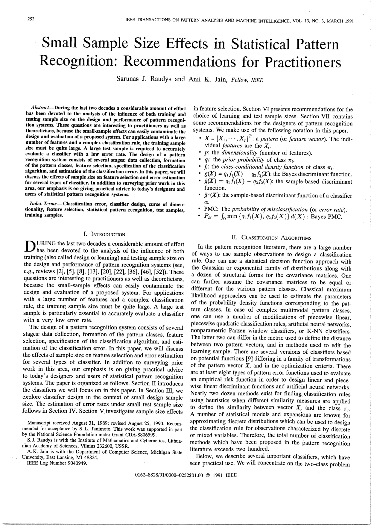
Small Sample Size Effects in Statistical Pattern Recognition: Recommendations for Practitioners

S. RaudysAnil K. Jain

article1991TPAMI1,489 citations

Presents practical guidelines and quantitative analyses to help practitioners choose appropriate training and test sample sizes, avoid small-sample bias in classifier design and feature selection, and accurately estimate classification error rates.

Listen

Organizations developing automated decision-making and machine learning systems frequently operate under data constraints where the number of training and testing examples is limited. In such environments, statistical models are prone to estimation errors that degrade classification accuracy and produce misleading performance evaluations. The article provides a comprehensive evaluation of how finite sample sizes impact classifier design, error estimation, and feature selection, delivering practical guidelines to help system designers balance data volume, algorithm complexity, and measurement reliability.

The authors analyze the mathematical and empirical properties of major parametric and nonparametric classification algorithms under finite data constraints. Combining analytical derivations based on multivariate statistical models with empirical simulations across artificial and real-world datasets, the article assesses error behavior across six standard classification rules: Euclidean distance, Fisher's linear discriminant, quadratic discriminant functions, Parzen window estimators, nearest neighbor rules, and multinomial classifiers.

The analysis establishes several vital findings regarding sample size requirements and model behavior. First, sample size demands scale sharply with classifier complexity: to limit the expected error increase to 50% or less over asymptotic optimal performance, linear classifiers require training sample sizes roughly proportional to the number of features, quadratic classifiers scale quadratically, and nonparametric kernel or histogram methods scale exponentially. Second, increasing the number of features without expanding the training data triggers a peaking effect, where classification accuracy initially improves but subsequently deteriorates due to parameter estimation error. Third, common performance metrics exhibit substantial distortion under small sample regimes; the resubstitution method systematically underestimates the true error rate, while feature selection based on small sample sizes leads to substantial optimistic bias, making suboptimal feature sets appear highly effective.

These findings indicate that deploying overly complex algorithms or indiscriminately expanding feature sets in data-limited environments introduces severe operational risk and performance degradation. Unbiased validation is critical; relying on uncorrected resubstitution or flawed feature evaluation creates an illusion of high model accuracy that fails in real-world deployment. Consequently, simpler models often outperform complex alternatives when data is scarce.

To mitigate these risks, practitioners should match classifier complexity strictly to available sample sizes, favoring robust linear discriminants when samples are small. For nonparametric algorithms, key tuning parameters—such as window widths and neighbor counts—must be systematically optimized. Teams should utilize resampling methods like cross-validation and bootstrap techniques to evaluate performance and explicitly compute estimation variance to establish confidence intervals. When choosing between training model parameters and validating results under a fixed total dataset, practitioners should allocate data using formal loss functions that balance training accuracy against test variance.

The article notes that its analytical formulas predominantly assume multivariate normal distributions with identical class covariances. While practical datasets frequently violate these ideal assumptions, the underlying qualitative principles provide robust engineering guidance. Readers should exercise caution when working with highly non-normal data or piecewise linear structures, and they should confirm system performance through rigorous empirical validation across competing algorithms.

Cover for Small Sample Size Effects in Statistical Pattern Recognition: Recommendations for Practitioners

Abstract

During the last two decades a considerable amount of effort has been devoted to the analysis of the influence of both training and testing sample size on the design and performance of pattern recognition systems. These questions are interesting to practitioners as well as theoreticians, because the small-sample effects can easily contaminate the design and evaluation of a proposed system. For applications with a large number of features and a complex classification rule, the training sample size must be quite large. A large test sample is required to accurately evaluate a classifier with a low error rate. The design of a pattern recognition system consists of several stages: data collection, formation of the pattern classes, feature selection, specification of the classification algorithm, and estimation of the classification error. In this paper, we will discuss the effects of sample size on feature selection and error estimation for several types of classifier. In addition to surveying prior work in this area, our emphasis is on giving practical advice to today's designers and users of statistical pattern recognition systems.

Table of Contents

  • I. INTRODUCTION
  • II. CLASSIFICATION ALGORITHMS
  • A. Euclidean Distance Classifier
  • B. Fisher's Linear Discriminant
  • C. Quadratic Discriminant Function
  • D. Parzen Window Classifier
  • E. K-Nearest-Neighbor (K-NN) Classifier
  • F. Multinomial Classifier
  • III. SENSITIVITY OF CLASSIFIERS TO DESIGN SAMPLE SIZE
  • IV. PERFORMANCE ESTIMATION
  • V. FEATURE SELECTION
  • A. Optimal Number of Features
  • B. Accuracy of Feature Selection
  • VI. SAMPLE SIZE DETERMINATION
  • VII. DISCUSSION
  • REFERENCES

Knowls

  1. Knowl 1 — Design Sample Size Requirements for Common Classifiers

    data/table

    To achieve a design where the expected probability of misclassification EPNEP_N is at most 1.51.5 times the asymptotic (infinite-sample) Bayes error P∞P_\infty (that is, EPN/P∞≤1.5EP_N / P_\infty \le 1.5), the total training sample size N=N1+N2N = N_1 + N_2 (with equal allocation N1=N2=N/2N_1 = N_2 = N/2) scales distinctly with dimensionality pp (or number of states mm) across different classification algorithms.

    Classifier Sample Size (N=N1=N2=N/2N = N_1 = N_2 = N/2) for P∞=0.10P_\infty = 0.10 Sample Size (N=N1=N2=N/2N = N_1 = N_2 = N/2) for P∞=0.01P_\infty = 0.01
    Euclidean (E) N=1.2pN = 1.2p N=1.6pN = 1.6p
    Fisher Linear (F) N=4.0pN = 4.0p N=9.0pN = 9.0p
    Quadratic (Q) N=10pN = 10p (p=8p=8), 16p16p (p=20p=20), 32p32p (p=50p=50) N=16pN = 16p (p=8p=8), 22p22p (p=20p=20), 40p40p (p=50p=50)
    Parzen Window (P, λ=0.8\lambda=0.8) N=4.4(1.77)pN = 4.4(1.77)^p N=30(1.55)pN = 30(1.55)^p
    Parzen Window (P, λ=0.1\lambda=0.1) N=60N = 60 (p=3p=3), N>100pN > 100p (p≥5p \ge 5) N=330N = 330 (p=3p=3), N≫100pN \gg 100p (p≥5p \ge 5)
    Multinomial (M, 10≤m≤10010 \le m \le 100) N=3.3mN = 3.3m N=5.0mN = 5.0m

    These results establish that:

    1. Linear classifiers (Euclidean and Fisher) require a training sample size that scales linearly with feature dimensionality pp.
    2. The quadratic discriminant classifier requires a sample size scaling quadratically with pp (i.e., N/pN/p grows linearly with pp).
    3. Nonparametric Parzen window classifiers require sample sizes that scale exponentially with feature dimensionality when the smoothing parameter λ\lambda is properly tuned to non-linear boundaries, though as λ→∞\lambda \to \infty the requirement converges to the linear Euclidean case.
    4. Discrete multinomial classifiers require sample size proportional to the number of multinomial states mm (which equals rpr^p if each of pp continuous features is discretized into rr bins).
  2. Knowl 2 — Asymptotic Decomposition of Classification Error Increase for Gaussian Parametric Classifiers

    theoretical result

    For two Gaussian pattern classes N(μ1,Σ1)\mathcal{N}(\mu_1, \Sigma_1) and N(μ2,Σ2)\mathcal{N}(\mu_2, \Sigma_2) with equal sample sizes N1=N2=N/2N_1 = N_2 = N/2, the asymptotic increase in expected probability of misclassification due to finite learning sample size NN is decomposed into additive penalty terms corresponding to each estimated parameter:

    ΔN=EPN−P∞≈1Nφ(δ/2)δ∑i∈Cαθi\Delta_N = EP_N - P_\infty \approx \frac{1}{N} \frac{\varphi(\delta/2)}{\delta} \sum_{i \in C_\alpha} \theta_i

    where φ(t)=(2π)−1/2e−t2/2\varphi(t) = (2\pi)^{-1/2} e^{-t^2/2} is the standard normal density, δ=(μ1−μ2)TΣ−1(μ1−μ2)\delta = \sqrt{(\mu_1 - \mu_2)^T \Sigma^{-1} (\mu_1 - \mu_2)} is the Mahalanobis distance, P∞=Φ(−δ/2)P_\infty = \Phi(-\delta/2) is the asymptotic Bayes error, and CαC_\alpha is the subset of parameter estimation terms required by classifier α\alpha.

    The parameter penalty terms θi\theta_i are defined as follows:

    • θ1=1\theta_1 = 1: Estimation of class prior probabilities q1,q2q_1, q_2.
    • θ2=δ24+p\theta_2 = \frac{\delta^2}{4} + p: Estimation of class mean vectors μ1,μ2\mu_1, \mu_2 in pp dimensions.
    • θ3=δ48+δ22\theta_3 = \frac{\delta^4}{8} + \frac{\delta^2}{2}: Estimation of common diagonal covariance variances (pp parameters).
    • θ4=δ48+3δ22+p\theta_4 = \frac{\delta^4}{8} + \frac{3\delta^2}{2} + p: Estimation of individual diagonal covariance variances (2p2p parameters).
    • θ5=δ44+pδ221−pN\theta_5 = \frac{\frac{\delta^4}{4} + \frac{p\delta^2}{2}}{1 - \frac{p}{N}}: Estimation of a common full covariance matrix Σ\Sigma (p(p+1)/2p(p+1)/2 parameters).
    • θ6=2(δ44+p(p+δ2)2)1−2pN\theta_6 = \frac{2\left(\frac{\delta^4}{4} + \frac{p(p+\delta^2)}{2}\right)}{1 - \frac{2p}{N}}: Estimation of separate full covariance matrices Σ1,Σ2\Sigma_1, \Sigma_2 (p(p+1)p(p+1) parameters).

    For the Euclidean distance classifier, CE={2}C_E = \{2\}. For Fisher's linear discriminant function, CF={1,2,5}C_F = \{1, 2, 5\}. For the quadratic discriminant function, CQ={1,2,6}C_Q = \{1, 2, 6\}.

  3. Knowl 3 — Three Types of Error and Selection Bias in Feature Subset Selection

    theoretical result

    When evaluating mm candidate feature subsets S1,…,SmS_1, \dots, S_m, sample-based feature evaluation induces optimistic selection bias. Three distinct errors characterize the selection process:

    1. Apparent error (P^apparent\hat{P}_{\text{apparent}}): The minimum sample-estimated error among all mm evaluated subsets: P^apparent=min⁡i=1,…,mP^i\hat{P}_{\text{apparent}} = \min_{i=1,\dots,m} \hat{P}_i
    2. Ideal error (PidealP_{\text{ideal}}): The minimum true error across all mm subsets: Pideal=min⁡i=1,…,mPiP_{\text{ideal}} = \min_{i=1,\dots,m} P_i
    3. True error of the chosen subset (PtrueP_{\text{true}}): The actual error of the subset selected by the algorithm (the one achieving the minimal sample estimate): Ptrue=Pi∗,where i∗=arg⁡min⁡i=1,…,mP^iP_{\text{true}} = P_{i^*}, \quad \text{where } i^* = \arg\min_{i=1,\dots,m} \hat{P}_i

    Because of sample variance in the estimates P^i\hat{P}_i, the ordering P^apparent<Pideal<Ptrue\hat{P}_{\text{apparent}} < P_{\text{ideal}} < P_{\text{true}} generally holds. The selection bias Δ1=Ptrue−P^apparent\Delta_1 = P_{\text{true}} - \hat{P}_{\text{apparent}} is approximately:

    Δ1≈kPmin⁡(1−Pmin⁡)nt\Delta_1 \approx k \sqrt{\frac{P_{\min}(1 - P_{\min})}{n_t}}

    where k∈[0.25,1.0]k \in [0.25, 1.0], Pmin⁡P_{\min} is the true error rate of the best subset, and ntn_t is the number of test samples used to compute each estimate P^i\hat{P}_i. The true error of the selected subset is related to the apparent error by:

    Ptrue≈P^apparent+2Δ1P_{\text{true}} \approx \hat{P}_{\text{apparent}} + 2\Delta_1

    As the number of searched subsets mm increases, Δ1\Delta_1 increases, so searching through larger numbers of candidate feature subsets without increasing test sample size ntn_t deteriorates the generalization performance of the selected subset.

  4. Knowl 4 — Nonparametric Estimation of Classifier Degradation and Asymptotic PMC

    model/method

    Because the learning curves for the expected resubstitution error EP^R=ϕ1(N)E\hat{P}_R = \phi_1(N) and the expected leave-one-out error EP^C=ϕ2(N)E\hat{P}_C = \phi_2(N) are approximately symmetric around the asymptotic classification error P∞P_\infty (P∞−EP^R≈EPN−P∞P_\infty - E\hat{P}_R \approx EP_N - P_\infty), the asymptotic error rate P∞P_\infty and the finite-sample performance increase ΔN=EPN−P∞\Delta_N = EP_N - P_\infty can be estimated nonparametrically without distributional assumptions:

    P^∞=P^C+P^R2\hat{P}_\infty = \frac{\hat{P}_C + \hat{P}_R}{2}

    Δ^N=P^C−P^R2\hat{\Delta}_N = \frac{\hat{P}_C - \hat{P}_R}{2}

    where P^C\hat{P}_C is the leave-one-out (cross-validation with k=1k=1) error estimate and P^R\hat{P}_R is the resubstitution error estimate evaluated on the NN training samples.

    Assuming P^C\hat{P}_C and P^R\hat{P}_R are approximately statistically independent, the mean squared error (MSE) of both estimates is given by:

    MSE(Δ^N)=MSE(P^∞)=12P^C(1−P^C)N+P^R(1−P^R)N\text{MSE}(\hat{\Delta}_N) = \text{MSE}(\hat{P}_\infty) = \frac{1}{2} \sqrt{\frac{\hat{P}_C(1 - \hat{P}_C)}{N} + \frac{\hat{P}_R(1 - \hat{P}_R)}{N}}

    If Δ^N\hat{\Delta}_N is small compared to P^∞\hat{P}_\infty, the design sample size NN is sufficient for the chosen classifier.

  5. Knowl 5 — Optimal Sample Partitioning between Training and Testing in Hold-Out

    model/method

    When a fixed total dataset of n∗n^* observations is partitioned into a training set of size N=N1+N2N = N_1 + N_2 and an independent test set of size nt=n∗−Nn_t = n^* - N, an optimal split balances classifier training degradation against error estimation variance. The total loss function is defined as:

    LOSS(N1,N2)=C1(EPN(N1,N2)−P∞)+C2MSE{P^(n∗−N1−N2)}\text{LOSS}(N_1, N_2) = C_1 (EP_N(N_1, N_2) - P_\infty) + C_2 \text{MSE}\{\hat{P}(n^* - N_1 - N_2)\}

    where C1C_1 and C2C_2 are application-specific cost weights for the finite-sample error increase and the estimator mean square error, respectively. For equal class splits (N1=N2=N/2N_1 = N_2 = N/2) and parametric linear classifiers, the finite-sample degradation is EPN−P∞=tα(P∞,p)NEP_N - P_\infty = \frac{t_\alpha(P_\infty, p)}{N}, and the standard error counting MSE is P^(1−P^)n∗−N\frac{\hat{P}(1-\hat{P})}{n^* - N}. Setting C1=C2=1C_1 = C_2 = 1 simplifies the loss to:

    LOSS(N)=tαN+P(1−P)n∗−N\text{LOSS}(N) = \frac{t_\alpha}{N} + \sqrt{\frac{P(1 - P)}{n^* - N}}

    where tα=N(EPN−P∞)t_\alpha = N(EP_N - P_\infty) is a classifier-dependent constant tabulated from asymptotic theory. Minimizing LOSS(N)\text{LOSS}(N) determines the optimal design sample size NN and test size nt=n∗−Nn_t = n^* - N.

  6. Knowl 6 — Minimum Test Sample Size for Required Classification Error Estimation Precision

    equation

    To guarantee with 2σ2\sigma (approximately 95%) confidence that the sample error counting estimate P^\hat{P} obtained from an independent test set of size ntn_t does not deviate from the true classification error PP by more than a relative error of k%k\% (that is, 2Var(P^)≤Pk1002\sqrt{\text{Var}(\hat{P})} \le \frac{P k}{100}), the minimum required test sample size is:

    nt≥4(1−P)P(k/100)2n_t \ge \frac{4(1 - P)}{P (k / 100)^2}

    where P∈(0,1)P \in (0, 1) is the true error rate of the classifier and k>0k > 0 is the percentage relative tolerance. For example, to achieve a relative precision of k=20%k = 20\% when the true error rate lies in the range 0.02≤P≤0.100.02 \le P \le 0.10, the required test sample size is between 900900 and 49004900 independent samples.

  7. Knowl 7 — Unbiased Quadratic Discriminant Function for Small Sample Sizes

    model/method

    Standard plug-in sample quadratic discriminant analysis (QDA) performs poorly in small sample regimes with unequal covariance matrices due to parameter estimation bias. Grabauskas's unbiased sample quadratic discriminant function corrects this bias analytically:

    g^QU(X)=∑j=12(−1)j+1{(1−pNj)(X−X‾(j))TSj−1(X−X‾(j))+ln⁡∣Sj∣qj−∑i=1pΨ(Nj−i2)+pln⁡Nj}\hat{g}^{QU}(X) = \sum_{j=1}^2 (-1)^{j+1} \left\{ \left(1 - \frac{p}{N_j}\right)(X - \overline{X}^{(j)})^T S_j^{-1}(X - \overline{X}^{(j)}) + \ln\frac{|S_j|}{q_j} - \sum_{i=1}^p \Psi\left(\frac{N_j - i}{2}\right) + p\ln N_j \right\}

    where X∈RpX \in \mathbb{R}^p is the feature vector to classify, NjN_j is the training sample size from class πj\pi_j, X‾(j)\overline{X}^{(j)} is the sample mean vector, SjS_j is the sample covariance matrix, qjq_j is the class prior probability, and Ψ(r)=ddrln⁡Γ(r)\Psi(r) = \frac{d}{dr}\ln\Gamma(r) is Euler's digamma function, computed via:

    Ψ(r+1)=−C+∑s=1r1s,Ψ(r+12)=−C−2ln⁡2+2∑s=1r11+2s\Psi(r + 1) = -C + \sum_{s=1}^r \frac{1}{s}, \quad \Psi\left(r + \frac{1}{2}\right) = -C - 2\ln 2 + 2\sum_{s=1}^r \frac{1}{1 + 2s}

    with Euler's constant C≈0.57721566C \approx 0.57721566.

    This discriminant function substantially lowers the expected misclassification rate relative to the standard plug-in quadratic rule when sample sizes N1N_1 and N2N_2 are small or unequal.

  8. Knowl 8 — Relative Variance of the Conditional Probability of Misclassification

    theoretical result

    For parametric linear classifiers (including Fisher's linear discriminant, logistic regression, and the Euclidean distance classifier) trained on finite samples, the increase in conditional probability of misclassification ΔN=PN−P∞\Delta_N = P_N - P_\infty follows a scaled chi-squared distribution:

    ΔN∼cχp2N\Delta_N \sim c \frac{\chi^2_p}{N}

    where pp is the feature dimensionality, NN is total sample size, and cc is a constant depending on asymptotic error P∞P_\infty and the classification rule.

    Consequently, the ratio of the standard deviation of the conditional probability of misclassification PNP_N to its expected excess error is inversely proportional to the square root of dimensionality:

    Var(PN)EPN−P∞=2p\frac{\sqrt{\text{Var}(P_N)}}{EP_N - P_\infty} = \sqrt{\frac{2}{p}}

    As dimensionality pp grows, the relative variability of the true conditional error across random training samples of size NN tends to zero, meaning PNP_N concentrates around its expectation EPNEP_N.

  9. Knowl 9 — Asymptotic Limits and Intrinsic Dimensionality Scaling of the Parzen Window Classifier

    theoretical result

    The Parzen window classifier discriminant function for classes π1,π2\pi_1, \pi_2 with kernel K(⋅)K(\cdot) and window width parameter λ\lambda:

    g^P(X)=q1N1∑i=1N1K(X−Xi(1)λ)−q2N2∑i=1N2K(X−Xi(2)λ)\hat{g}^P(X) = \frac{q_1}{N_1} \sum_{i=1}^{N_1} K\left(\frac{X - X_i^{(1)}}{\lambda}\right) - \frac{q_2}{N_2} \sum_{i=1}^{N_2} K\left(\frac{X - X_i^{(2)}}{\lambda}\right)

    exhibits two limiting behaviors for exponential or logistic kernels:

    1. As λ→∞\lambda \to \infty, a Taylor series expansion reveals that the decision boundary converges to a linear classifier: g^P(X)→gE(X)+tr(S2)−tr(S1)\hat{g}^P(X) \to g^E(X) + \text{tr}(S_2) - \text{tr}(S_1) where gE(X)=2[X−12(X‾(1)+X‾(2))]T(X‾(1)−X‾(2))g^E(X) = 2\left[X - \frac{1}{2}(\overline{X}^{(1)} + \overline{X}^{(2)})\right]^T (\overline{X}^{(1)} - \overline{X}^{(2)}) is the Euclidean distance discriminant and tr(Si)\text{tr}(S_i) is the trace of the class sample covariance matrix. In this regime, the required design sample size scales as O(1/N)O(1/N).
    2. As λ→0\lambda \to 0, the decision boundary becomes highly nonlinear and coincides with the 1-nearest neighbor (1-NN) classification rule.

    Furthermore, when the same smoothing parameter λ\lambda is used across all normalized features, the design sample size required for a specified accuracy scales exponentially with the intrinsic dimensionality p∗p^* (N=αβp∗N = \alpha \beta^{p^*}) rather than the nominal feature dimension pp.

  10. Knowl 10 — Peaking Phenomenon and Optimal Dimensionality in Finite-Sample Classifiers

    theoretical result

    In finite-sample pattern recognition, adding features decreases asymptotic Bayes error P∞P_\infty, but increases the variance of parameter estimates. This trade-off produces a non-monotonic learning curve where expected misclassification error EPN(p)EP_N(p) first drops, achieves a global minimum at an optimal dimensionality poptp_{\text{opt}}, and then increases with additional features (the peaking phenomenon).

    When features are equally effective or added in random order under multivariate normal distributions:

    1. For Fisher's linear discriminant with NN independent training samples across both classes, the optimal number of features is approximately: popt≈N2−1p_{\text{opt}} \approx \frac{N}{2} - 1
    2. For the quadratic discriminant function, poptp_{\text{opt}} is substantially lower than N/2−1N/2 - 1 due to the O(p2)O(p^2) parameters in class covariance matrices, but grows monotonically with NN.
    3. When features are ordered a priori by decreasing discriminative power, EPN(p)EP_N(p) exhibits a relatively flat valley around poptp_{\text{opt}}, making the exact choice of poptp_{\text{opt}} less critical than avoiding severe over-dimensionality (p≫poptp \gg p_{\text{opt}}).

Coverage note — None was omitted; the knowls cover all core contributions including sample size rules of thumb, Gaussian error breakdowns, feature selection biases, error estimation variance and nonparametric bounds, optimal data splitting, unbiased QDA, Parzen asymptotic limits, and the peaking phenomenon.

References

  1. 1.R. A. Abusev and Y. P. Lumelskij, "Unbiased estimators and classification problems for multivariate normal populations," Theor. Prob. and Appl., vol. 25, pp. 381-389, 1980 (in Russian).
  2. 2.S. A. Aivazian, V. M. Buchstaber, I. S. Yenyukov, and L. D. Meshalkin, "Applied statistics: Classification and reduction of dimensionality," Finansy i Statistika (Reference Edition), Moscow, 1989 (in Russian).
  3. 3.B. G. Batchelor and D. J. Hand, "Pattern recognition competition," in Proc. 3rd Int. Conf. Pattern Recognition, Coronado, 1976, pp. 315-321.
  4. 4.M. Ben-Bassat, "Use of distance measures, information measures and error bounds in feature evaluation," in Handbook of Statistics, vol. 2, P. R. Krishnaiah and L. N. Kanal, Eds. Amsterdam, The Netherlands: North-Holland, 1982, pp. 773-791.
  5. 5.L. Breiman, J. Friedman, R. A. Olsen, and C. J. Stone, Classifica-tion and Regression Trees. Belmont, CA: Wadsworth, 1984.
  6. 6.Y. D. Broffitt, "Nonparametric classification," in Handbook of Statistics, vol. 2, P. R. Krishnaiah and L. N. Kanal, Eds. Amsterdam, The Netherlands: North-Holland, 1982, pp. 139-168.
  7. 7.B. Chandrasekaran and A. K. Jain, "On balancing decision functions," J. Cybern. Inform. Sci., vol. 2, pp. 12-15, 1979.
  8. 8.L. Devroye and T. J. Wagner, "Nearest neighbor methods in discrimination," in Handbook of Statistics, vol. 2, P. R. Krishnaiah and L. N. Kanal, Eds. Amsterdam, The Netherlands: North-Holland, 1982, pp. 193-198.
  9. 9.R. O. Duda and P. E. Hart, Pattern Classification and Scene Analysis. New York: Wiley, 1973.
  10. 10.B. Efron, "The efficiency of logistic regression compared to normal discriminant analysis," J. Amer. Statist. Assoc., vol. 70, pp. 892-898, 1975.
  11. 11.I. S. Enukov, "A choice of a set of measurements with maximal discriminating power in the case of limited learning sample size," in Multivariate Statistical Analysis in Social-Economic Research. Moscow, USSR: Nauka, 1974, pp. 394-397 (in Russian).
  12. 12.D. M. Foley, "Considerations of sample and feature size," IEEE Trans. Inform. Theory, vol. IT-18, pp. 618-626, 1972.
  13. 13.K. Fukunaga, "Statistical pattern recognition," in Handbook of Pattern Recognition and Image Processing, T. Y. Young and K. S. Fu, Eds. New York: Academic, 1986, pp. 3-32.
  14. 14.K. Fukunaga and L. D. Hostetler, "Optimization of K-nearest neighbor density estimates," IEEE Trans. Inform. Theory, vol. IT-19, pp. 320-326, 1973.
  15. 15.S. Geiser, "Posterior odds for multivariate normal classifications," J. Roy. Statist. Soc. B, vol. 21, no. 1, pp. 69-76, 1964.
  16. 16.N. Glick, "Additive estimators for probabilities of correct classification," Pattern Recog., vol. 10, no. 3, pp. 211-222, 1978.
  17. 17.M. Goldstein and W. R. Dillon, Discrete Discriminant Analysis. New York: Wiley, 1978.
  18. 18.V. Grabauskas, Inst. Math. Cybern., Acad. Sci., Lithuania, personal communication, 1983.
  19. 19.D. Griškevičius and Š. Raudys, "On the expected probability of the classification error of the classifier for discrete variables," in Statistical Problems of Control, issue 38, Š. Raudys, Ed. Vilnius, USSR: Inst. Math. Cybern. Press, 1979, pp. 95-112 (in Russian).
  20. 20.D. J. Hand, "Recent advances in error rate estimation," Pattern Recog. Lett., vol. 5, pp. 335-346, 1986.
  21. 21.A. K. Jain, R. C. Dubes, and C. C. Chen, "Bootstrap techniques for error estimation," IEEE Trans. Pattern Anal. Machine Intell., vol. PAMI-9, no. 9, pp. 628-636, 1987.
  22. 22.A. K. Jain and B. Chandrasekaran, "Dimensionality and sample size considerations in pattern recognition practice," in Handbook of Statistics, vol. 2, P. R. Krishnaiah and L. N. Kanal, Eds. Amsterdam, The Netherlands, North-Holland, 1982, pp. 835-855.
  23. 23.A. K. Jain and M. D. Ramaswami, "Classifier design with Parzen windows," in Pattern Recognition and Artificial Intelligence, E. S. Gelsema and L. N. Kanal, Eds. Amsterdam, The Netherlands: Elsevier, 1988, pp. 211-228.
  24. 24.A. K. Jain and W. G. Waller, "On the optimal number of features in the classification of multivariate Gaussian data," Pattern Recog., vol. 10, pp. 365-374, 1978.
  25. 25.L. Kanal, "Patterns in pattern recognition 1968-1974," IEEE Trans. Inform. Theory, vol. IT-20, pp. 697-722, 1974.
  26. 26.L. Kanal and B. Chandrasekaran, "On dimensionality and sample size in statistical pattern classification," Pattern Recog., vol. 3, pp. 238-255, 1971.
  27. 27.D. G. Keehn, "A note on learning for Gaussian properties," IEEE Trans. Inform. Theory, vol. IT-11, no. 1, pp. 126-131, 1965.
  28. 28.J. Kittler, "Feature selection and extraction," in Handbook of Pattern Recognition and Image Processing, T. Y. Young and K. S. Fu, Eds. New York: Academic, 1986, pp. 60-83.
  29. 29.P. A. Lachenbruch and R. M. Mickey, "Estimation of error rates in discriminant analysis," Technometrics, vol. 10, no. 1, pp. 1-11, 1968.
  30. 30.P. A. Lachenbruch, C. Sneeringer, and L. T. Revo, "Robustness of the linear and quadratic discriminant functions to certain types of non-normality," Commun. Statist., vol. 1, no. 1, pp. 39-56, 1972.
  31. 31.G. S. Lbov, "Logical functions in the problems of empirical prediction," in Handbook of Statistics, vol. 2, P. R. Krishnaiah and L. N. Kanal, Eds. Amsterdam, The Netherlands: North-Holland, 1982, pp. 479-491.
  32. 32.T. Lissack and K. S. Fu, "Error estimation in pattern recognition via L-distance between posterior density functions," IEEE Trans. Inform. Theory, vol. IT-22, pp. 34-45, 1976.
  33. 33.G. J. McLachlan, "The bias of the apparent error rate in discriminant analysis," Biometrika, vol. 63, pp. 239-244, 1976.
  34. 34.------, "Assessing the performance of an allocation rule," Comput. Math. Applicat., vol. 12A, pp. 261-272, 1976.
  35. 35.------, "The efficiency of Efron's 'bootstrap' approach to error estimation in discriminant analysis," J. Stat. Comput. Simulation, vol. 11, pp. 273-279, 1980.
  36. 36.------, "Error rate estimation in discriminant analysis: Recent advances," in Advances in Multivariate Statistical Analysis, A. K. Gupta, Ed. Dordrect, The Netherlands: Reidel, 1987, pp. 233-252.
  37. 37.L. Miroshnichenko, "Comparison of algorithms for selecting the best feature set in pattern recognition," in Statistical Problems of Control, issue 93. Vilnius, USSR: Inst. Math. Cybern. Press, 1990, pp. 78-91 (in Russian).
  38. 38.T. Y. O'Neill, "The general distribution of the error rate of a classification procedure with application to logistic regression discrimination," J. Amer. Statist. Assoc., vol. 75, pp. 154-160, 1980.
  39. 39.K. W. Pettis, T. A. Bailey, A. K. Jain, and R. C. Dubes, "An intrinsic dimensionality estimator from near-neighbor information," IEEE Trans. Pattern Anal. Machine Intell., vol. PAMI-1, no. 1, pp. 25-37, 1979.
  40. 40.V. Pikelis, "Analysis of learning speed of three linear classifiers," Ph.D. dissertation, Inst. Phys. Math., Vilnius, pp. 1-136, 1974 (in Russian).
  41. 41.Š. Raudys, "On the problems of sample size in pattern recognition," in Proc. 2nd All-Union Conf. Statistical Methods in Control Theory, Moscow, USSR: Nauka, 1970, pp. 64-67 (in Russian).
  42. 42.Š. Raudys, V. Pikelis, and K. Juškevičius, "Experimental comparison of thirteen classification algorithms," in Statistical Problems of Control, issue 11, Vilnius, USSR: Inst. Phys. Math. Press, 1975, pp. 35-80 (in Russian).
  43. 43.Š. Raudys, "Comparison of the estimates of the probability of misclassification," in Proc. 4th Int. Conf. Pattern Recognition, Kyoto, Japan, Nov. 1978, pp. 280-282.
  44. 44.------, "Determination of optimal dimensionality in statistical pattern classification," Pattern Recog., vol. 11, pp. 263-270, 1979.
  45. 45.Š. Raudys and V. Pikelis, "On dimensionality, sample size, classification error, and complexity of classification algorithm in pattern recognition," IEEE Trans. Pattern Anal. Machine Intell., vol. PAMI-2, no. 3, pp. 242-252, 1980.
  46. 46.Š. Raudys, "The influence of sample size on classification performance," in Statistical Problems of Control, issue 66. Vilnius, USSR, Inst. Math. Cybern. Press, 1984, pp. 9-42 (in Russian).
  47. 47.Š. Raudys and V. Vaitukaitis, "Methods to estimate the probability of misclassification," in Statistical Problems of Control, issue 66. Vilnius, USSR: Inst. Math. Cybern. Press, 1984, pp. 43-65 (in Russian).
  48. 48.Š. Raudys, "On the accuracy of a bootstrap estimate of the classification error," in Proc. 9th Int. Conf. Pattern Recognition, Rome, Italy, Nov. 1988, pp. 1230-1232.
  49. 49.Š. Raudys, V. Pikelis, and D. Stasaitis, "The effects of the number of initial and final features, the dependence between the features and the type of a classification rule on the accuracy of feature selection," Pattern Recog. Artificial Intell., 1990, submitted for publication.
  50. 50.J. W. Sayre, "The distribution of actual error rates in linear discriminant analysis," J. Amer. Statist. Assoc., vol. 75, pp. 201-205, 1980.
  51. 51.I. K. Sethi and G. P. R. Sarvarayudu, "Hierarchical classifier design using mutual information," IEEE Trans. Pattern Anal. Machine Intell., vol. PAMI-4, pp. 441-445, 1982.
  52. 52.M. Siotani, "Large sample approximations and asymptotic expansions of classification statistics," in Handbook of Statistics, vol. 2, P. R. Krishnaiah and L. N. Kanal, Eds. Amsterdam, The Netherlands: North-Holland, 1982, pp. 61-100.
  53. 53.M. Skurikhina, "Effect of the kernel form on the quality of nonparametric Parzen window classifier," in Statistical Problems of Control, issue 93. Vilnius, USSR: Inst, Math. Cybern. Press, 1990 (in Russian).
  54. 54.G. T. Toussaint, "Bibliography on estimation of misclassification," IEEE Trans. Inform. Theory, vol. 20; pp. 472-479, 1974.
  55. 55.N. Vanichsetakul, "Tree structured classification via recursive discriminant analysis," Ph.D. dissertation, Univ. Wisconsin, 1986.
  56. 56.V. N. Vapnik, Recovery of Dependencies from Empirical Data. New York: Springer-Verlag, 1982.
  57. 57.C. T. Wolverton and T. J. Wagner, "Asymptotically optimal discriminant functions for pattern classification," IEEE Trans. Inform. Theory, vol. IT-15, no. 2, pp. 258-265, 1969.
  58. 58.D. Žvirėnaitė, "Criteria for selecting the informative features in pattern recognition," in Statistical Problems of Control, issue 74. Vilnius, USSR: Inst. Math. Cybern. Press, 1986, pp. 76-103 (in Russian).

Citation

MLA
Raudys, S. J., and A. K. Jain. “Small Sample Size Effects in Statistical Pattern Recognition: Recommendations for Practitioners”. IEEE Transactions on Pattern Analysis and Machine Intelligence, vol. 13, no. 3, 1991, pp. 252–64, https://doi.org/10.1109/34.75512.
APA
Raudys, S. J., & Jain, A. K. (1991). Small sample size effects in statistical pattern recognition: recommendations for practitioners. IEEE Transactions on Pattern Analysis and Machine Intelligence, 13(3), 252–264. https://doi.org/10.1109/34.75512
Chicago
Raudys, S. J., and A. K. Jain. 1991. “Small Sample Size Effects in Statistical Pattern Recognition: Recommendations for Practitioners”. IEEE Transactions on Pattern Analysis and Machine Intelligence 13 (3): 252–64. https://doi.org/10.1109/34.75512.
Harvard
Raudys, S.J. and Jain, A.K. (1991) “Small sample size effects in statistical pattern recognition: recommendations for practitioners”, IEEE Transactions on Pattern Analysis and Machine Intelligence, 13(3), pp. 252–264. Available at: https://doi.org/10.1109/34.75512.
Vancouver
1. Raudys SJ, Jain AK (1991) Small sample size effects in statistical pattern recognition: recommendations for practitioners. IEEE Transactions on Pattern Analysis and Machine Intelligence 13:252–264

BibTeX

@article{Raudys_1991, title={Small sample size effects in statistical pattern recognition: recommendations for practitioners}, volume={13}, ISSN={0162-8828}, url={http://dx.doi.org/10.1109/34.75512}, DOI={10.1109/34.75512}, number={3}, journal={IEEE Transactions on Pattern Analysis and Machine Intelligence}, publisher={Institute of Electrical and Electronics Engineers (IEEE)}, author={Raudys, S.J. and Jain, A.K.}, year={1991}, month=Mar, pages={252–264} }
Metadata:Crossref

Access the Paper

This paper is available from its original source. Click below to access the PDF.

Open PDF