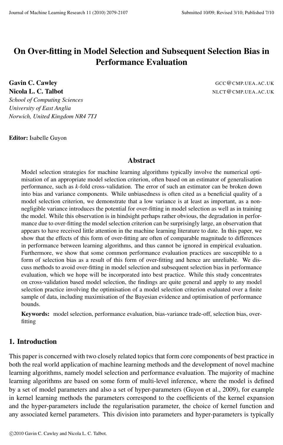
On Over-fitting in Model Selection and Subsequent Selection Bias in Performance Evaluation

G. CawleyN. L. C. Talbot

article2010JMLR2,471 citations

Demonstrates that hyperparameter tuning on finite datasets can cause severe overfitting during model selection, introducing substantial optimistic bias into performance evaluations and requiring nested cross-validation for reliable algorithm comparisons.

Listen

In real-world machine learning applications, selecting high-level configuration settings—known as hyper-parameters—is essential for optimizing model accuracy. While practitioners widely recognize the danger of a model memorizing noise during initial training, the article addresses a less recognized problem: tuning hyper-parameters against finite validation datasets can lead to a second layer of over-fitting during the model selection phase itself. This issue often results in misleadingly optimistic performance estimates when deploying models in production or comparing competing algorithms.

The article sets out to demonstrate how the statistical variability of model selection criteria causes this second-level over-fitting and evaluates how common performance evaluation workflows introduce significant selection bias. To demonstrate this, the authors evaluated standard classification algorithms—primarily kernel ridge regression and Gaussian process classifiers—using synthetic benchmarks with known optimal error rates alongside a standard suite of thirteen real-world benchmark datasets partitioned across up to one hundred distinct data splits.

The analysis revealed several critical findings. First, optimizing hyper-parameters against finite validation datasets initially improves generalization, but continuing optimization degrades test performance as the search tunes to sample-specific statistical noise. Second, having more hyper-parameters to tune makes models substantially more vulnerable to this failure; for example, simpler models with a single shared parameter statistically outperformed flexible models with feature-specific parameters across twelve of the thirteen benchmark datasets. Third, widespread evaluation shortcuts—such as selecting hyper-parameters on a preliminary data subset and applying their median value across all test partitions, or tuning hyper-parameters on the full dataset before cross-validation—introduce an artificial optimistic bias ranging up to roughly 1.0 to 1.2 percentage points in error rates. Crucially, this artificial bias is often larger than the actual performance differences between competing machine learning models.

These findings indicate that reported benchmark leads in technical literature may frequently be artifacts of flawed testing protocols rather than genuine algorithmic superiority. Shortcut workflows conceal performance degradation and unfairly favor unstable selection methods over more robust designs. For organizations building predictive models, trusting flawed validation metrics introduces operational and financial risk by delivering production models that underperform expectations.

To ensure reliable results, organizations should mandate rigorous nested evaluation workflows where model selection is treated as an inseparable part of training and repeated entirely within each data split. Flawed shortcut protocols—such as pre-tuning hyper-parameters or fixing median parameters across test folds—should be deprecated. When tuning complex models on small datasets, teams should implement variance-reduction strategies such as regularizing hyper-parameters, applying early stopping, or utilizing fully Bayesian parameter averaging. While these nested evaluations require greater computational power, the parallelizable nature of the workflows and modern computing architectures make rigorous validation entirely practical.

University of East Anglia bayesian methods cross validation evaluation models Overfit in Model Selection Select Bias in Performance Evaluation Cross‑Validate

Cawley et al (2010).pdf

Paper: A survey of cross-validation procedures for model selection, Sylvain Arlot et al. (2009). This survey provides a comprehensive theoretical and empirical foundation on the bias and variance trade-offs in cross-validation procedures that the source builds upon when evaluating selection bias.
Paper: A Study of Cross-Validation and Bootstrap for Accuracy Estimation and Model Selection, Ron Kohavi (1995). It establishes fundamental empirical benchmarks for cross-validation and bootstrap accuracy estimation in model selection, directly informing the evaluation pitfalls studied in the source.
Paper: Choosing Multiple Parameters for Support Vector Machines, OLIVIER CHAPELLE et al. (2002). It details how tuning multiple hyper-parameters simultaneously impacts generalization error bounds and optimization, which the source critically re-evaluates in the context of over-fitting during model selection.
Paper: Stability and Generalization, Olivier Bousquet et al. (2002). It formalizes algorithmic stability and its theoretical connection to generalization bounds, underpinning the source's analysis of how unstable model selection rules introduce optimism bias.
Paper: Approximate Statistical Tests for Comparing Supervised Classification Learning Algorithms, Thomas G. Dietterich (1998). It analyzes statistical testing procedures and false-positive rates when comparing supervised classifiers across validation folds, laying the groundwork for addressing selection bias in benchmark comparisons.

Paper: Random Search for Hyper-Parameter Optimization, James Bergstra et al. (2012). It demonstrates how randomized search mitigates the computational and over-fitting traps of exhaustive multi-parameter tuning exposed in the source.
Paper: Practical Bayesian Optimization of Machine Learning Algorithms, Jasper Snoek et al. (2012). It applies a fully Bayesian optimization treatment to hyperparameter selection, directly implementing the parameter averaging and variance-reduction strategies suggested by the source.
Paper: Making a Science of Model Search: Hyperparameter Optimization in Hundreds of Dimensions for Vision Architectures, J. Bergstra et al. (2013). It extends systematic hyperparameter search across hundreds of architecture dimensions while confronting the question of whether reported benchmark gains stem from genuine algorithmic improvements or intensive tuning.
Paper: Hyperband: A Novel Bandit-Based Approach to Hyperparameter Optimization, Lisha Li et al. (2016). It introduces a bandit-based framework for resource allocation in hyperparameter optimization that incorporates early stopping to improve search efficiency and guard against over-fitting.
Paper: Deep Reinforcement Learning at the Edge of the Statistical Precipice, Rishabh Agarwal et al. (2021). It extends the critique of flawed evaluation protocols and aggregate metrics to modern deep reinforcement learning benchmarks.
Paper: Deep Reinforcement Learning that Matters, Peter Henderson et al. (2018). It empirically examines reproducibility issues and optimistic reporting biases caused by hyperparameter tuning and random seeds across machine learning algorithms.
Paper: Do we need hundreds of classifiers to solve real world classification problems?, Manuel Fernández Delgado et al. (2014). It conducts a large-scale standardized benchmark of classifiers to test whether algorithmic performance claims hold up under controlled, uniform cross-validation splits.
Paper: On Hyperparameter Optimization of Machine Learning Algorithms: Theory and Practice, Li Yang et al. (2020). It provides a broad retrospective survey of modern hyperparameter optimization strategies and software workflows developed to handle high-dimensional tuning effectively.

Cover for On Over-fitting in Model Selection and Subsequent Selection Bias in Performance Evaluation

Abstract

Model selection strategies for machine learning algorithms typically involve the numerical optimisation of an appropriate model selection criterion, often based on an estimator of generalisation performance, such as k-fold cross-validation. The error of such an estimator can be broken down into bias and variance components. While unbiasedness is often cited as a beneficial quality of a model selection criterion, we demonstrate that a low variance is at least as important, as a non-negligible variance introduces the potential for over-fitting in model selection as well as in training the model. While this observation is in hindsight perhaps rather obvious, the degradation in performance due to over-fitting the model selection criterion can be surprisingly large, an observation that appears to have received little attention in the machine learning literature to date. In this paper, we show that the effects of this form of over-fitting are often of comparable magnitude to differences in performance between learning algorithms, and thus cannot be ignored in empirical evaluation. Furthermore, we show that some common performance evaluation practices are susceptible to a form of selection bias as a result of this form of over-fitting and hence are unreliable. We discuss methods to avoid over-fitting in model selection and subsequent selection bias in performance evaluation, which we hope will be incorporated into best practice. While this study concentrates on cross-validation based model selection, the findings are quite general and apply to any model selection practice involving the optimisation of a model selection criterion evaluated over a finite sample of data, including maximisation of the Bayesian evidence and optimisation of performance bounds.

2. Kernel Ridge Regression
2.1 Efficient Leave-One-Out Cross-Validation
3. Data Sets used in Empirical Demonstrations
3.1 A Synthetic Benchmark
3.2 A Suite of Benchmarks for Robust Performance Evaluation
4. Over-fitting in Model Selection
4.1 Bias and Variance in Model Selection
4.2 The Effects of Over-fitting in Model Selection
4.3 Is Over-fitting in Model Selection Really a Genuine Concern in Practice?
4.4 Avoiding Over-fitting in Model Selection
5. Bias in Performance Estimation
5.1 An Unbiased Performance Evaluation Methodology
5.2 An Example of Biased Evaluation Methodology
5.2.1 IS THE BIAS SOLELY DUE TO INADVERTENT RE-USE OF TEST SAMPLES?
5.2.2 IS THE MEDIAN PROTOCOL INTERNALLY CONSISTENT?
5.3 Another Example of Biased Evaluation Methodology
6. Conclusions
Acknowledgments
References

Knowls

Knowl 1 — Over-fitting in Model Selection
definition
Over-fitting in model selection refers to the phenomenon where a model selection criterion (such as $k$ -fold cross-validation error, leave-one-out cross-validation error, split-sample validation error, or negative marginal likelihood/Bayesian evidence), evaluated over a finite sample of training data $\mathcal{D}$ , is numerically optimized beyond the point where the true generalization performance of the model improves, causing the true test error to subsequently increase.

While over-fitting at the first level of inference (parameter training) occurs when model parameters over-fit empirical training loss, over-fitting at the second level of inference (hyperparameter selection) arises because empirical model selection criteria $g(\theta; \mathcal{D})$ are sample-based estimators of the true generalization function $G(\theta)$ . When the estimator $g(\theta; \mathcal{D})$ exhibits non-negligible variance across different sample realizations of $\mathcal{D}$ , numerical optimization of $g(\theta; \mathcal{D})$ with respect to hyperparameters $\theta$ exploits sample-specific random peculiarities rather than true underlying structure.
Knowl 2 — Bias-Variance Decomposition of Model Selection Criteria
equation
Let $G(\theta)$ denote the true generalization error of a machine learning model indexed by hyperparameter vector $\theta \in \Theta$ , and let $g(\theta; \mathcal{D})$ denote an estimator of generalization error computed over a finite sample $\mathcal{D}$ of $n$ observations. The expected squared error of the model selection estimator across independent realizations of datasets $\mathcal{D}$ of size $n$ decomposes into squared bias and variance components:

$\mathbb{E}_{\mathcal{D}}\left[ (g(\theta; \mathcal{D}) - G(\theta))^2 \right] = \left( \mathbb{E}_{\mathcal{D}}[g(\theta; \mathcal{D})] - G(\theta) \right)^2 + \mathbb{E}_{\mathcal{D}}\left[ \left( g(\theta; \mathcal{D}) - \mathbb{E}_{\mathcal{D}'}[g(\theta; \mathcal{D}')] \right)^2 \right]$

In the context of hyperparameter optimization, the objective is to locate the optimal hyperparameter $\theta^* = \arg\min_\theta G(\theta)$ . While an unbiased estimator ensures that $\mathbb{E}_{\mathcal{D}}[g(\theta; \mathcal{D})] = G(\theta)$ , on any single finite sample $\mathcal{D}_i$ the model selection procedure minimizes $g(\theta; \mathcal{D}_i)$ . A high variance term $\mathbb{E}_{\mathcal{D}}[ (g(\theta; \mathcal{D}) - \mathbb{E}[g(\theta; \mathcal{D})])^2 ]$ causes large scatter in the location of the empirical minimizer $\hat{\theta} = \arg\min_\theta g(\theta; \mathcal{D}_i)$ , leading to over-fitting in model selection. Consequently, a biased estimator with low variance can produce hyperparameter estimates closer to $\theta^*$ than an unbiased estimator with high variance.
Knowl 3 — Closed-Form Leave-One-Out Residuals and PRESS Statistic for Kernel Ridge Regression
model/method
In kernel ridge regression (KRR) for classification or regression with training data $\mathcal{D} = \{(\mathbf{x}_i, y_i)\}_{i=1}^\ell$ where $\mathbf{x}_i \in \mathbb{R}^d$ and $y_i \in \{-1, +1\}$ , the decision function is $f(\mathbf{x}) = \sum_{i=1}^\ell \alpha_i K(\mathbf{x}_i, \mathbf{x}) + b$ . The dual parameter vector $\boldsymbol{\alpha} = (\alpha_1, \dots, \alpha_\ell)^T$ and bias $b$ are obtained by solving the linear system:

$\begin{bmatrix} \mathbf{K} + \lambda \mathbf{I} & \mathbf{1} \\ \mathbf{1}^T & 0 \end{bmatrix} \begin{bmatrix} \boldsymbol{\alpha} \\ b \end{bmatrix} = \begin{bmatrix} \mathbf{y} \\ 0 \end{bmatrix}$

where $\mathbf{K} \in \mathbb{R}^{\ell \times \ell}$ is the kernel matrix with entries $K_{ij} = K(\mathbf{x}_i, \mathbf{x}_j)$ , $\mathbf{I}$ is the $\ell \times \ell$ identity matrix, $\mathbf{1} = (1, \dots, 1)^T \in \mathbb{R}^\ell$ , $\mathbf{y} = (y_1, \dots, y_\ell)^T$ , and $\lambda > 0$ is the regularization parameter.

Let $\mathbf{C} = \begin{bmatrix} \mathbf{K} + \lambda \mathbf{I} & \mathbf{1} \\ \mathbf{1}^T & 0 \end{bmatrix}$ . The leave-one-out residual for the $i$ -th training pattern when trained on the remaining $\ell - 1$ samples is given in closed form without explicit retraining by:

$r_i^{(-i)} = y_i - \hat{y}_i^{(-i)} = \frac{\alpha_i}{[\mathbf{C}^{-1}]_{ii}}$

where $[\mathbf{C}^{-1}]_{ii}$ denotes the $i$ -th diagonal element of the inverse matrix $\mathbf{C}^{-1}$ . Allen's Predicted Residual Sum-of-Squares (PRESS) statistic for hyperparameters $\boldsymbol{\theta} = (\lambda, \boldsymbol{\eta})$ is computed as:

$\text{PRESS}(\boldsymbol{\theta}) = \sum_{i=1}^\ell \left[ r_i^{(-i)} \right]^2 = \sum_{i=1}^\ell \left( \frac{\alpha_i}{[\mathbf{C}^{-1}]_{ii}} \right)^2$
Knowl 4 — Empirical Demonstration of Model Selection Over-fitting on Nested RBF and ARD Kernels
empirical result
When comparing isotropic Radial Basis Function (RBF) kernels: $K_{\text{RBF}}(\mathbf{x}, \mathbf{x}') = \exp\left( -\eta \|\mathbf{x} - \mathbf{x}'\|^2 \right)$ and Automatic Relevance Determination (ARD) Gaussian kernels with dimension-specific scaling parameters: $K_{\text{ARD}}(\mathbf{x}, \mathbf{x}') = \exp\left( -\sum_{j=1}^d \eta_j (x_j - x'_j)^2 \right)$ the isotropic RBF model is structurally nested inside the ARD model family as the special case $\eta_1 = \dots = \eta_d = \eta$ . In principle, the optimal generalization achievable by an ARD kernel must equal or exceed that of the RBF kernel.

However, empirical evaluation across 13 benchmark datasets (with sample sizes $\ell \in [140, 1300]$ and feature dimensions $d \in [2, 60]$ ) shows the opposite:
1. In Kernel Ridge Regression (KRR) tuned via the PRESS statistic, the RBF kernel achieves statistically significantly lower test error rates on 8 of 13 datasets, whereas ARD achieves superiority on only 1 (image). Across nearly all benchmarks, ARD achieves lower PRESS values on the training data than RBF while exhibiting higher test errors.
2. In Expectation-Propagation Gaussian Process Classifiers (EP-GPC) tuned by maximizing marginal likelihood, RBF achieves statistically significantly lower test error on 6 benchmarks, whereas ARD is superior on only 2 (image and splice). ARD consistently yields higher marginal likelihood on training data despite worse test generalization.
This confirms that increasing hyperparameter degrees of freedom increases the variance of the model selection criterion, exacerbating over-fitting in model selection and degrading test generalization.

Knowl 5 — Error Rates and Selection Criteria for Isotropic RBF versus ARD Kernels

data/table

The tables below compare the test error rates and model selection criteria for Kernel Ridge Regression (KRR, tuned by minimizing PRESS) and Expectation-Propagation Gaussian Process Classifiers (EP-GPC, tuned by minimizing negative log-evidence, $-\log \text{Evidence}$ ) across 13 benchmark datasets over 100 random realizations (20 for image and splice). Bold values indicate statistically superior error rates or significantly better selection criteria.

Data Set	KRR RBF Test Error	KRR ARD Test Error	KRR RBF PRESS	KRR ARD PRESS
banana	$10.610 \pm 0.051$	$10.638 \pm 0.052$	$60.808 \pm 0.636$	$60.957 \pm 0.624$
breast cancer	$\mathbf{26.727 \pm 0.466}$	$28.766 \pm 0.391$	$70.632 \pm 0.328$	$\mathbf{66.789 \pm 0.385}$
diabetis	$\mathbf{23.293 \pm 0.169}$	$24.520 \pm 0.215$	$146.143 \pm 0.452$	$\mathbf{141.465 \pm 0.606}$
flare solar	$34.140 \pm 0.175$	$34.375 \pm 0.175$	$267.332 \pm 0.480$	$\mathbf{263.858 \pm 0.550}$
german	$\mathbf{23.540 \pm 0.214}$	$25.847 \pm 0.267$	$228.256 \pm 0.666$	$\mathbf{221.743 \pm 0.822}$
heart	$\mathbf{16.730 \pm 0.359}$	$22.810 \pm 0.411$	$42.576 \pm 0.356$	$\mathbf{37.023 \pm 0.494}$
image	$2.990 \pm 0.159$	$\mathbf{2.188 \pm 0.134}$	$74.056 \pm 1.685$	$\mathbf{44.488 \pm 1.222}$
ringnorm	$\mathbf{1.613 \pm 0.015}$	$2.750 \pm 0.042$	$28.324 \pm 0.246$	$\mathbf{27.680 \pm 0.231}$
splice	$10.777 \pm 0.144$	$9.943 \pm 0.520$	$186.814 \pm 2.174$	$\mathbf{130.888 \pm 6.574}$
thyroid	$4.747 \pm 0.235$	$4.693 \pm 0.202$	$9.099 \pm 0.152$	$\mathbf{6.816 \pm 0.164}$
titanic	$22.483 \pm 0.085$	$22.562 \pm 0.109$	$48.332 \pm 0.622$	$\mathbf{47.801 \pm 0.623}$
twonorm	$\mathbf{2.846 \pm 0.021}$	$4.292 \pm 0.086$	$\mathbf{32.539 \pm 0.279}$	$35.620 \pm 0.490$
waveform	$\mathbf{9.792 \pm 0.045}$	$11.836 \pm 0.085$	$61.658 \pm 0.596$	$\mathbf{56.424 \pm 0.637}$

Data Set	EP-GPC RBF Test Error	EP-GPC ARD Test Error	EP-GPC RBF $-\log\text{Ev}$	EP-GPC ARD $-\log\text{Ev}$
banana	$\mathbf{10.413 \pm 0.046}$	$10.459 \pm 0.049$	$116.894 \pm 0.917$	$\mathbf{116.459 \pm 0.923}$
breast cancer	$\mathbf{26.506 \pm 0.487}$	$27.948 \pm 0.492$	$110.628 \pm 0.366$	$\mathbf{107.181 \pm 0.388}$
diabetis	$\mathbf{23.280 \pm 0.182}$	$23.853 \pm 0.193$	$230.211 \pm 0.553$	$\mathbf{222.305 \pm 0.581}$
flare solar	$34.200 \pm 0.175$	$\mathbf{33.578 \pm 0.181}$	$394.697 \pm 0.546$	$\mathbf{384.374 \pm 0.512}$
german	$\mathbf{23.363 \pm 0.211}$	$23.757 \pm 0.217$	$359.181 \pm 0.778$	$\mathbf{346.048 \pm 0.835}$
heart	$\mathbf{16.670 \pm 0.290}$	$19.770 \pm 0.365$	$73.464 \pm 0.493$	$\mathbf{67.811 \pm 0.571}$
image	$2.817 \pm 0.121$	$\mathbf{2.188 \pm 0.076}$	$205.061 \pm 1.687$	$\mathbf{123.896 \pm 1.184}$
ringnorm	$\mathbf{4.406 \pm 0.064}$	$8.589 \pm 0.097$	$121.260 \pm 0.499$	$\mathbf{91.356 \pm 0.583}$
splice	$11.609 \pm 0.180$	$\mathbf{8.618 \pm 0.924}$	$365.208 \pm 3.137$	$\mathbf{242.464 \pm 16.980}$
thyroid	$4.373 \pm 0.219$	$\mathbf{4.227 \pm 0.216}$	$25.461 \pm 0.182$	$\mathbf{18.867 \pm 0.170}$
titanic	$\mathbf{22.637 \pm 0.134}$	$22.725 \pm 0.133$	$78.952 \pm 0.670$	$\mathbf{78.373 \pm 0.683}$
twonorm	$\mathbf{3.060 \pm 0.034}$	$4.025 \pm 0.068$	$45.901 \pm 0.577$	$\mathbf{42.044 \pm 0.610}$
waveform	$\mathbf{10.100 \pm 0.047}$	$11.418 \pm 0.091$	$105.925 \pm 0.954$	$\mathbf{91.239 \pm 0.962}$

The data demonstrate that ARD models regularly achieve better training selection metrics (lower PRESS and lower negative log-evidence) but significantly worse test error rates.

Knowl 6 — The Internal Performance Evaluation Protocol
algorithm
To prevent selection bias in performance evaluation, model selection (hyperparameter tuning) and model training (parameter estimation) must be executed as an inseparable joint pipeline independently for every trial or fold of a resampling procedure.
Input: Dataset $D$ , outer fold count $K_{\text{out}}$ , inner fold count $K_{\text{in}}$ , hyperparameter space $\Theta$
Output: Unbiased generalization error estimate $\bar{E}$
Partition $D$ into $K_{\text{out}}$ disjoint folds $\{D_1, D_2, \dots, D_{K_{\text{out}}}\}$
for $k = 1$ to $K_{\text{out}}$ do
    Set test partition $D_{\text{test}}^{(k)} = D_k$
    Set training partition $D_{\text{train}}^{(k)} = D \setminus D_k$
    Perform model selection using only $D_{\text{train}}^{(k)}$ :
         $\hat{\theta}^{(k)} = \arg\min_{\theta \in \Theta} g(\theta; D_{\text{train}}^{(k)})$ using $K_{\text{in}}$ -fold CV, leave-one-out, or marginal likelihood
    Fit model parameters $\hat{\mathbf{w}}^{(k)}$ on $D_{\text{train}}^{(k)}$ using hyperparameters $\hat{\theta}^{(k)}$
    Evaluate error $E_k = \text{Loss}(\hat{\mathbf{w}}^{(k)}, \hat{\theta}^{(k)}; D_{\text{test}}^{(k)})$
end for
return $\bar{E} = \frac{1}{K_{\text{out}}} \sum_{k=1}^{K_{\text{out}}} E_k$
In this nested protocol, test samples in $D_{\text{test}}^{(k)}$ remain strictly unseen during both parameter optimization and hyperparameter selection.

Knowl 7 — Optimistic Selection Bias Induced by the Median Hyperparameter Protocol

empirical result

The median protocol is an evaluation heuristic where model selection is performed on only the first 5 realizations of a benchmark dataset to obtain candidate hyperparameter sets $\boldsymbol{\theta}_1, \dots, \boldsymbol{\theta}_5$ . The coordinate-wise median $\tilde{\boldsymbol{\theta}} = \text{median}(\boldsymbol{\theta}_1, \dots, \boldsymbol{\theta}_5)$ is then fixed and evaluated across all 100 data realizations.

Evaluating Kernel Ridge Regression (RBF-KRR) across 13 benchmark datasets reveals that the median protocol introduces an optimistic bias (underestimating test error) on 11 of 13 datasets:

Data Set	KRR (Internal)	KRR (Median)	Bias (Internal - Median)
banana	$10.610 \pm 0.051$	$10.384 \pm 0.042$	$+0.226 \pm 0.034$
breast cancer	$26.727 \pm 0.466$	$26.377 \pm 0.441$	$+0.351 \pm 0.195$
diabetis	$23.293 \pm 0.169$	$23.150 \pm 0.157$	$+0.143 \pm 0.074$
flare solar	$34.140 \pm 0.175$	$34.013 \pm 0.166$	$+0.128 \pm 0.082$
german	$23.540 \pm 0.214$	$23.380 \pm 0.220$	$+0.160 \pm 0.067$
heart	$16.730 \pm 0.359$	$15.720 \pm 0.306$	$+1.010 \pm 0.186$
image	$2.990 \pm 0.159$	$2.802 \pm 0.129$	$+0.188 \pm 0.095$
ringnorm	$1.613 \pm 0.015$	$1.573 \pm 0.010$	$+0.040 \pm 0.010$
splice	$10.777 \pm 0.144$	$10.763 \pm 0.137$	$+0.014 \pm 0.055$
thyroid	$4.747 \pm 0.235$	$4.560 \pm 0.200$	$+0.187 \pm 0.100$
titanic	$22.483 \pm 0.085$	$22.407 \pm 0.102$	$+0.076 \pm 0.077$
twonorm	$2.846 \pm 0.021$	$2.868 \pm 0.017$	$-0.022 \pm 0.014$
waveform	$9.792 \pm 0.045$	$9.821 \pm 0.039$	$-0.029 \pm 0.020$

For datasets such as heart ( $+1.010\%$ ) and breast cancer ( $+0.351\%$ ), the bias exceeds the difference in performance between competing classifiers evaluated under the internal protocol, falsely indicating statistical superiority under Wilcoxon signed ranks tests ( $p < 0.05$ ).

Knowl 8 — Mechanisms and Inconsistency of Bias in the Median Protocol
empirical result
The optimistic bias of the median hyperparameter evaluation protocol arises from three factors:
1. Data re-use: Training instances from the first 5 folds appear in test partitions of other realizations.
2. Hyperparameter variance reduction: The median operation across 5 folds acts as a variance reduction step, producing a hyperparameter vector with lower estimation variance than any single fold's selected hyperparameters.
3. Suppression of fold-specific over-fitting: Using fixed hyperparameters prevents the model selection procedure from over-fitting each realization's specific training partition.
In a controlled synthetic experiment using 100 independent realizations (64 training samples and a mutually disjoint 4096-sample test set, strictly eliminating data re-use), taking the median of hyperparameters over 5 folds still produced a statistically significant optimistic bias ( $p < 0.001$ , Wilcoxon signed ranks test).

Furthermore, the magnitude of the bias differs significantly across learning algorithms (e.g., Wilcoxon test on bias differences between KRR and EP-GPC yielded $p < 0.05$ on 5 of 13 benchmarks). When varying the number of folds in a repeated split-sample model selection procedure, the median protocol introduced the largest optimistic bias when the model selection variance was highest (fewest folds), thereby disguising poor model selection procedures and distorting relative algorithm rankings.

Knowl 9 — Optimistic Selection Bias in the External Cross-Validation Protocol

empirical result

In the "external" performance evaluation protocol, model selection is performed once on the entire dataset to determine fixed hyperparameters $\boldsymbol{\theta}^*$ , followed by 10-fold cross-validation with those fixed hyperparameters. Because the test samples in every fold were included in the initial model selection step, the hyperparameters retain a memory of the test data.

Evaluating Kernel Ridge Regression with an RBF kernel across 13 benchmark datasets shows that the external protocol yields consistently optimistic error estimates compared to the internal protocol:

Data Set	External Error (%)	Internal Error (%)	Bias (%)
banana	$10.355 \pm 0.146$	$10.495 \pm 0.158$	$+0.140 \pm 0.035$
breast cancer	$26.280 \pm 0.232$	$27.470 \pm 0.250$	$+1.190 \pm 0.135$
diabetis	$22.891 \pm 0.127$	$23.056 \pm 0.134$	$+0.165 \pm 0.050$
flare solar	$34.518 \pm 0.172$	$34.707 \pm 0.179$	$+0.189 \pm 0.051$
german	$23.999 \pm 0.117$	$24.217 \pm 0.125$	$+0.219 \pm 0.045$
heart	$16.335 \pm 0.214$	$16.571 \pm 0.220$	$+0.235 \pm 0.073$
image	$3.081 \pm 0.102$	$3.173 \pm 0.112$	$+0.092 \pm 0.035$
ringnorm	$1.567 \pm 0.058$	$1.607 \pm 0.057$	$+0.040 \pm 0.014$
splice	$10.930 \pm 0.219$	$11.170 \pm 0.280$	$+0.240 \pm 0.152$
thyroid	$3.743 \pm 0.137$	$4.279 \pm 0.152$	$+0.536 \pm 0.073$
titanic	$22.167 \pm 0.434$	$22.487 \pm 0.442$	$+0.320 \pm 0.077$
twonorm	$2.480 \pm 0.067$	$2.502 \pm 0.070$	$+0.022 \pm 0.021$
waveform	$9.613 \pm 0.168$	$9.815 \pm 0.183$	$+0.203 \pm 0.064$

The optimistic bias is statistically significant ( $\text{bias} > 2 \times \text{SE}$ ) on 11 of 13 datasets (all except splice and twonorm). On datasets like breast cancer ( $+1.190\%$ ) and thyroid ( $+0.536\%$ ), the bias is large enough to conceal genuine differences between competitive and uncompetitive learning algorithms even when optimizing only two hyperparameters.

Knowl 10 — Techniques for Mitigating Over-fitting in Model Selection
model/method
When sample sizes are limited and collecting additional data is not possible, over-fitting of the model selection criterion can be addressed using several methodological strategies:
1. Regularization of the model selection criterion: Incorporating explicit prior distributions or penalty terms over the hyperparameter space $\Theta$ to penalize extreme values during numerical optimization (e.g., Bayesian regularization of hyperparameters).
2. Early stopping in hyperparameter optimization: Halting the numerical minimization of the model selection criterion prior to convergence, preventing the optimizer from exploiting high-frequency statistical noise in the validation sample.
3. Hyperparameter averaging / Model averaging: Combining predictions across a distribution of candidate hyperparameter settings rather than committing to a single point-estimate minimizer $\hat{\boldsymbol{\theta}}$ .
4. Fully Bayesian integration: Integrating out hyperparameters via Markov Chain Monte Carlo (MCMC) or analytical approximations rather than performing numerical point optimization.
5. Constraining hyperparameter degrees of freedom: Restricting the hyperparameter search dimensionality (such as using isotropic kernel functions with a single shared bandwidth instead of Automatic Relevance Determination kernels) or optimizing feature weights at the inner training level under a single global regularization hyperparameter.

Coverage note — No substantial contributed material was omitted from the extracted knowls.

References

1.D. M. Allen. The relationship between variable selection and prediction. Technometrics, 16:125–127, 1974.
2.C. Ambroise and G. J. McLachlan. Selection bias in gene extraction on the basis of microarray gene-expression data. Proceedings of the National Academy of Sciences, 99(10):6562–6566, May 14 2002. doi: 10.1073/pnas.102102699.
3.S. An, W. Liu, and S. Venkatesh. Fast cross-validation algorithms for least squares support vector machines and kernel ridge regression. Pattern Recognition, 40(8):2154–2162, August 2007. doi: 10.1016/j.patcog.2006.12.015.
4.E. Andelić, M. Schafföner, M. Katz, S. E. Krüger, and A. Wendermuth. Kernel least-squares models using updates of the pseudoinverse. Neural Computation, 18(12):2928–2935, December 2006. doi: 10.1162/neco.2006.18.12.2928.
5.Y. Bengio and Y. Grandvalet. No unbiased estimator of the variance of k-fold cross-validation. Journal of Machine Learning Research, 5:1089–1105, 2004.
6.S. A. Billings and K. L. Lee. Nonlinear Fisher discriminant analysis using a minimum squared error cost function and the orthogonal least squares algorithm. Neural Networks, 15(2):263–270, March 2002. doi: 10.1016/S0893-6080(01)00142-3.
7.C. M. Bishop. Neural Networks for Pattern Recognition. Oxford University Press, 1995.
8.L. Bo, L. Wang, and L. Jiao. Feature scaling for kernel Fisher discriminant analysis using leave-one-out cross validation. Neural Computation, 18(4):961–978, April 2006. doi: 10.1162/neco.2006.18.4.961.
9.O. Bousquet and A. Elisseeff. Stability and generalization. Journal of Machine Learning Research, 2:499–526, 2002.
10.L. Breiman. Random forests. Machine Learning, 45(1):5–32, October 2001. doi: 10.1023/A:1010933404324.
11.G. C. Cawley. Leave-one-out cross-validation based model selection criteria for weighted LS-SVMs. In Proceedings of the IEEE/INNS International Joint Conference on Neural Networks (IJCNN-06), pages 1661–1668, Vancouver, BC, Canada, July 16–21 2006. doi: 10.1109/IJCNN.2006.246634.
12.G. C. Cawley and N. L. C. Talbot. Efficient leave-one-out cross-validation of kernel Fisher discriminant classifiers. Pattern Recognition, 36(11):2585–2592, November 2003. doi: 10.1016/S0031-3203(03)00136-5.
13.G. C. Cawley and N. L. C. Talbot. Preventing over-fitting during model selection via Bayesian regularisation of the hyper-parameters. Journal of Machine Learning Research, 8:841–861, April 2007.
14.G. C. Cawley and N. L. C. Talbot. Efficient approximate leave-one-out cross-validation for kernel logistic regression. Machine Learning, 71(2–3):243–264, June 2008. doi: 10.1007/s10994-008-5055-9.
15.G. C. Cawley, G. J. Janacek, and N. L. C. Talbot. Generalised kernel machines. In Proceedings of the IEEE/INNS International Joint Conference on Neural Networks (IJCNN-07), pages 1720–1725, Orlando, Florida, USA, August 12–17 2007. doi: 10.1109/IJCNN.2007.4371217.
16.O. Chapelle, V. Vapnik, O. Bousquet, and S. Mukherjee. Choosing multiple parameters for support vector machines. Machine Learning, 46(1–3):131–159, January 2002. doi: 10.1023/A:1012450327387.
17.H. Chen, P. Tino, and X. Yao. Probabilistic classification vector machines. IEEE Transactions on Neural Networks, 20(6):901–914, June 2009. doi: 10.1109/TNN.2009.2014161.
18.W. Chu, S. S. Keerthi, and C. J. Ong. Bayesian trigonometric support vector classifier. Neural Computation, 15(9):2227–2254, September 2003. doi: 10.1162/089976603322297368.
19.J. Demšar. Statistical comparisons of classifiers over multiple data sets. Journal of Machine Learning Research, 7:1–30, 2006.
20.R. O. Duda, P. E. Hart, and D. G. Stork. Pattern Classification. John Wiley and Sons, second edition, 2001.
21.B. Efron and R. J. Tibshirani. Introduction to the Bootstrap. Monographs on Statistics and Applied Probability. Chapman & Hall, 1994.
22.S. Geman, E. Bienenstock, and R. Doursat. Neural networks and the bias/variance dilemma. Neural Computation, 4(1):1–58, January 1992. doi: 10.1162/neco.1992.4.1.1.
23.C. Gold, A. Holub, and P. Sollich. Bayesian approach to feature selection and parameter tuning for support vector machine classifiers. Neural Networks, 18(5):693–701, July/August 2005. doi: 10.1016/j.neunet.2005.06.044.
24.I. Guyon, A. Saffari, G. Dror, and G. Cawley. Model selection: Beyond the Bayesian/frequentist divide. Journal of Machine Learning Research, 11:61–87, 2009.
25.P. Hall and A. P. Robinson. Reducing the variability of crossvalidation for smoothing parameter choice. Biometrika, 96(1):175–186, March 2009. doi: doi:10.1093/biomet/asn068.
26.M. Kearns and D. Ron. Algorithmic stability and sanity-check bounds for leave-one-out cross-validation. Neural Computation, 11(6):1427–1453, August 1999. doi: 10.1162/089976699300016304.
27.G. S. Kimeldorf and G. Wahba. Some results on Tchebycheffian spline functions. Journal of Mathematical Analysis and Applications, 33:82–95, 1971.
28.S. R. Kulkarni, G. Lugosi, and S. S. Venkatesh. Learning pattern classification — a survey. IEEE Transactions on Information Theory, 44(6):2178–2206, October 1998.
29.P. A. Lachenbruch and M. R. Mickey. Estimation of error rates in discriminant analysis. Technometrics, 10(1):1–12, February 1968.
30.A. Luntz and V. Brailovsky. On estimation of characters obtained in statistical procedure of recognition (in Russian). Techicheskaya Kibernetica, 3, 1969.
31.D. J. C. MacKay. Bayesian interpolation. Neural Computation, 4(3):415–447, May 1992. doi: 10.1162/neco.1992.4.3.415.
32.J. Mercer. Functions of positive and negative type and their connection with the theory of integral equations. Philosophical Transactions of the Royal Society of London, Series A, 209:415–446, 1909.
33.S. Mika, G. Rätsch, J. Weston, B. Schölkopf, and K.-R. Müller. Fisher discriminant analysis with kernels. In Neural Networks for Signal Processing IX, Proceedings of the 1999 IEEE Signal Processing Society Workshop, pages 41–48, Maddison, WI, USA, 21–25 August 1999. doi: 10.1109/NNSP.1999.788121.
34.S. Mika, G. Rätsch, J. Weston, B. Schölkpf, and K.-R. Müller. Contructing descriptive and discriminative nonlinear features: Rayleigh coefficients in kernel feature spaces. IEEE Transactions on Pattern Analysis and Machine Intelligence, 25(5):623–628, May 2003. doi: 10.1109/TPAMI.2003.1195996.
35.J. A. Nelder and R. Mead. A simplex method for function minimization. Computer Journal, 7:308–313, 1965.
36.T. Peña Centeno and Lawrence N. D. Optimising kernel parameters and regularisation coefficients for non-linear discriminant analysis. Journal of Machine Learning Research, 7:455–491, February 2006.
37.T. Poggio and F. Girosi. Networks for approximation and learning. Proceedings of the IEEE, 78(9):1481–1497, September 1990. doi: 10.1109/5.58326.
38.Y. Qi, T. P. Minka, R. W. Picard, and Z. Ghahramani. Predictive automatic relevance determination by expectation propagation. In Proceedings of the Twenty First International Conference on Machine Learning (ICML-04), pages 671–678, Banff, Alberta, Canada, July 4–8 2004.
39.C. E. Rasmussen and C. K. I. Williams. Gaussian Processes for Machine Learning. Adaptive Computation and Machine Learning. MIT Press, 2006.
40.G. Rätsch, T. Onoda, and K.-R. Müller. Soft margins for AdaBoost. Machine Learning, 42(3):287–320, March 2001. doi: 10.1023/A:1007618119488.
41.R. M. Rifkin and R. A. Lippert. Notes on regularized least squares. Technical Report MIT-CSAIL-TR-2007-025, Computer Science and Artificial Intelligence Laboratory, MIT, May 2007.
42.B. D. Ripley. Pattern Recognition and Neural Networks. Cambridge University Press, 1996.
43.C. Saunders, A. Gammerman, and V. Vovk. Ridge regression learning algorithm in dual variables. In Proceedings of the Fifteenth International Conference on Machine Learning (ICML-98), pages 515–521. Morgan Kaufmann, 1998.
44.J. Shao. Linear model selection by cross-validation. Journal of the American Statistical Society, 88:486–494, 1993.
45.I. Stewart. On the optimal parameter choice for ν-support vector machines. IEEE Transactions on Pattern Analysis and Machine Intelligence, 25(10):1274–1284, October 2003. doi: 10.1109/TPAMI.2003.1233901.
46.M. Stone. Cross-validatory choice and assessment of statistical predictions. Journal of the Royal Statistical Society, Series B (Statistical Methodology), 36(2):111–147, 1974.
47.M. Stone. Asymptotics for and against cross-validation. Biometrika, 64(1):29–35, April 1977. doi: 10.1093/biomet/64.1.29.
48.J. A. K. Suykens, T. Van Gestel, J. De Brabanter, B. De Moor, and J. Vanderwalle. Least Squares Support Vector Machine. World Scientific Publishing Company, Singapore, 2002. ISBN 981-238-151-1.
49.A. N. Tikhonov and V. Y. Arsenin. Solutions of Ill-posed Problems. John Wiley, New York, 1977.
50.G. Toussaint. Bibliography on estimation of misclassification. IEEE Transactions on Information Theory, IT-20(4):472–479, July 1974.
51.V. N. Vapnik. Estimation of Dependences Based on Empirical Data. Springer, 1982.
52.V. N. Vapnik. Statistical Learning Theory. Adaptive and learning systems for signal processing, communications and control series. Wiley, 1998.
53.S. Weisberg. Applied Linear Regression. Probability and Mathematical Statistics. John Wiley & Sons, second edition, 1985.
54.J. Weston. Leave-one-out support vector machines. In Proceedings of the Sixteenth International Joint Conference on Artificial Intelligence (IJCAI-99), pages 727–733, San Fransisco, CA, USA, 1999. Morgan Kaufmann.
55.C. K. I. Williams and D. Barber. Bayesian classification with Gaussian processes. IEEE Transactions on Pattern Analysis and Machine Intelligence, 20(12):1342–1351, December 1998. doi: 10.1109/34.735807.
56.P. M. Williams. A Marquardt algorithm for choosing the step size in backpropagation learning with conjugate gradients. Technical Report CSRP-229, University of Sussex, February 1991.
57.T. Zhang. Leave-one-out bounds for kernel machines. Neural Computation, 15(6):1397–1437, June 2003. doi: 10.1162/089976603321780326.

Citation

MLA

Cawley, G. C., and N. L. C. Talbot. “On Over-fitting in Model Selection and Subsequent Selection Bias in Performance Evaluation”. Journal of Machine Learning Research, vol. 11, no. 70, 2010, pp. 2079–107, https://www.jmlr.org/papers/v11/cawley10a.html.

APA

Cawley, G. C., & Talbot, N. L. C. (2010). On Over-fitting in Model Selection and Subsequent Selection Bias in Performance Evaluation. Journal of Machine Learning Research, 11(70), 2079–2107. https://www.jmlr.org/papers/v11/cawley10a.html

Chicago

Cawley, G. C., and N. L. C. Talbot. 2010. “On Over-fitting in Model Selection and Subsequent Selection Bias in Performance Evaluation”. Journal of Machine Learning Research 11 (70): 2079–2107. https://www.jmlr.org/papers/v11/cawley10a.html.

Harvard

Cawley, G.C. and Talbot, N.L.C. (2010) “On Over-fitting in Model Selection and Subsequent Selection Bias in Performance Evaluation”, Journal of Machine Learning Research, 11(70), pp. 2079–2107. Available at: https://www.jmlr.org/papers/v11/cawley10a.html.

Vancouver

1. Cawley GC, Talbot NLC (2010) On Over-fitting in Model Selection and Subsequent Selection Bias in Performance Evaluation. Journal of Machine Learning Research 11:2079–2107

BibTeX

@article{JMLR:v11:cawley10a,
  author  = {Gavin C. Cawley and Nicola L. C. Talbot},
  title   = {On Over-fitting in Model Selection and Subsequent Selection Bias in Performance Evaluation},
  journal = {Journal of Machine Learning Research},
  year    = {2010},
  volume  = {11},
  number  = {70},
  pages   = {2079--2107},
  url     = {http://jmlr.org/papers/v11/cawley10a.html}
}

Metadata:DOI registry

Access the Paper

This paper is available from its original source. Click below to access the PDF.

Open PDF

License: https://creativecommons.org/licenses/by/4.0/

On Over-fitting in Model Selection and Subsequent Selection Bias in Performance Evaluation

Abstract

Topics

Keywords

Table of Contents

Knowls

Knowl 1 — Over-fitting in Model Selection

Knowl 2 — Bias-Variance Decomposition of Model Selection Criteria

Knowl 3 — Closed-Form Leave-One-Out Residuals and PRESS Statistic for Kernel Ridge Regression

Knowl 4 — Empirical Demonstration of Model Selection Over-fitting on Nested RBF and ARD Kernels