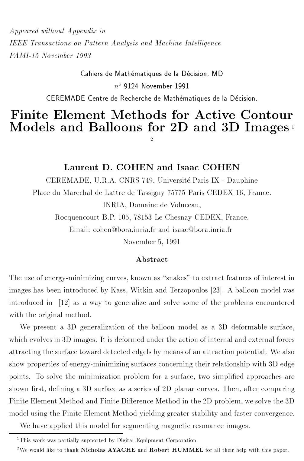
Finite-Element Methods for Active Contour Models and Balloons for 2-D and 3-D Images

L. CohenI. Cohen

article1993TPAMI1,663 citations

Presents a three-dimensional generalization of the balloon deformable surface model and implements a finite element framework that achieves faster convergence and superior numerical stability for volumetric medical image segmentation.

Listen

Extracting accurate boundaries and 3D geometric surfaces of anatomical structures from medical imaging—such as magnetic resonance imaging (MRI)—is a vital step in computer-assisted diagnosis, surgical planning, and quantitative measurement. Traditional active contour models (commonly known as "snakes") often fail in practical clinical settings because they are overly sensitive to initial placement, easily trapped by image noise or spurious edges, and computationally demanding when scaled to volumetric data.

The article develops and evaluates an enhanced deformable model framework that extends 2D active contours to true 3D deformable surfaces. It demonstrates how incorporating inflation and weight forces, integrating prior edge detection into attraction potentials, and applying finite element numerical methods provide a robust, automated method for segmenting complex anatomical objects.

The authors implemented the approach across both synthetic geometric data and real-world medical scans, including 3D MRI data of heart ventricles and human craniofacial anatomy. They compared simplified slice-by-slice 3D approximations with full 3D active surface formulations solved via the Finite Element Method (FEM) using Bogner-Fox-Schmit rectangular elements, contrasting these directly with traditional Finite Difference Methods (FDM).

Key findings include:

The introduction of internal pressure ("balloon") and directional "weight" forces prevents the model from collapsing, enables it to bypass isolated spurious noise, and allows convergence from simple, coarse initializations located far from the true target.
The Finite Element Method reduces the size of the required linear system by roughly nine times compared to finite differences (requiring node spacing around one-sixth the contour length rather than one node per pixel), yielding lower algorithmic complexity, greater numerical stability, and faster convergence without needing dynamic node additions.
True 3D deformable surface models successfully bridge large gaps and reconstruct missing edge data across successive image slices, whereas 2D slice-by-slice approaches fail under identical missing-data conditions.
The resulting continuous, analytical surface description provides direct access to differential properties, such as mean curvature and fundamental forms, which are critical for subsequent shape analysis and feature extraction.

These results demonstrate that the full 3D FEM deformable model substantially lowers operator intervention, mitigates segmentation failure risks caused by noisy or incomplete scan data, and delivers smooth, mathematically usable 3D organ surfaces. While full 3D FEM surface extraction requires approximately ten times more computation time than simplified 2D stack methods, the dramatic gain in reconstruction fidelity and robustness justifies the cost for complex anatomical targets.

For practical adoption, organizations and research teams should implement the full 3D FEM active surface framework for high-precision volumetric segmentation where slice-to-slice continuity is critical, while reserving faster, simplified slice-by-slice models for simpler cylindrical structures. Next steps include developing adaptive triangular meshes for arbitrary surface topologies and applying the reconstructed surfaces to atlas matching and automatic landmark identification. Users should note that parameter choices for elasticity and rigidity must be properly calibrated to ensure numerical stability and avoid over-smoothing fine structural details.

CEREMADE INRIA Paris Dauphine University computational efficiency edge detection feature extraction Active Contour Models Finite-Element Methods deformable surfaces

Cohen et al (1993).pdf

Paper: Marching cubes: A high resolution 3D surface construction algorithm, William E. Lorensen et al. (1987). This seminal work introduces the Marching Cubes algorithm for extracting 3D surface meshes directly from volumetric medical data, providing foundational context for representing and extracting 3D volumetric surfaces.
Paper: Surface reconstruction from unorganized points, Hugues Hoppe et al. (1992). This foundational paper establishes techniques for surface reconstruction and continuous implicit geometry extraction, directly preceding the geometric formulation of 3D active surfaces.
Paper: Decimation of triangle meshes, William J. Schroeder et al. (1992). This paper develops mesh decimation algorithms for simplifying volumetric isosurface models, establishing essential principles for efficient polygonal representations used in 3D medical modeling.
Paper: Free-form deformation of solid geometric models, Thomas W. Sederberg et al. (1986). This work introduces free-form deformation techniques for solid geometric models, laying foundational geometric mechanics for deformable surface modeling.

Paper: Region Competition: Unifying Snakes, Region Growing, and Bayes/MDL for Multiband Image Segmentation, Song Chun Zhu et al. (1996). This work unifies classic snake and balloon models with statistical region growing and Bayesian estimation under an energy-minimization framework for robust image segmentation.
Paper: Shape Modeling with Front Propagation: A Level Set Approach, R. Malladi et al. (1995). This paper extends active contour segmentation by embedding front propagation in a level set framework to handle complex topology changes without the mesh parametrization constraints of FEM snakes.
Paper: A Multiphase Level Set Framework for Image Segmentation Using the Mumford and Shah Model, Luminita A. Vese et al. (2002). This work advances variational active contour and surface models into a multiphase level set approach based on the Mumford-Shah functional to segment complex multi-region images.
Paper: A signal processing approach to fair surface design, Gabriel Taubin (1995). This paper presents non-shrinking signal-processing algorithms to fair and smooth 3D polyhedral surface meshes extracted from volumetric medical data.
Paper: Implicit fairing of irregular meshes using diffusion and curvature flow, Mathieu Desbrun et al. (1999). This study develops implicit curvature flow and scale-dependent Laplacian methods for fairing irregular 3D meshes, advancing the numerical treatment of extracted surface geometry.
Paper: Graph Cuts and Efficient N-D Image Segmentation, Yuri Boykov et al. (2006). This paper provides a discrete, globally optimal combinatorial alternative to continuous active contour and balloon models for N-dimensional volumetric medical segmentation.
Paper: Random Walks for Image Segmentation, Leo Grady (2006). This article formulates interactive 2D and 3D image segmentation using discrete Dirichlet random walks as an alternative to traditional continuous deformable models.
Paper: A volumetric method for building complex models from range images, Brian Curless et al. (1996). This work builds on volumetric surface reconstruction principles to integrate continuous signed-distance fields into seamless, watertight 3D models.

Cover for Finite-Element Methods for Active Contour Models and Balloons for 2-D and 3-D Images

Abstract

The use of energy-minimizing curves, known as "snakes" to extract features of interest in images has been introduced by Kass, Witkin and Terzopoulos [23]. A balloon model was introduced in [12] as a way to generalize and solve some of the problems encountered with the original method.

We present a 3D generalization of the balloon model as a 3D deformable surface, which evolves in 3D images. It is deformed under the action of internal and external forces attracting the surface toward detected edgels by means of an attraction potential. We also show properties of energy-minimizing surfaces concerning their relationship with 3D edge points. To solve the minimization problem for a surface, two simplified approaches are shown first, defining a 3D surface as a series of 2D planar curves. Then, after comparing Finite Element Method and Finite Difference Method in the 2D problem, we solve the 3D model using the Finite Element Method yielding greater stability and faster convergence.

We have applied this model for segmenting magnetic resonance images.

Topics

computational efficiency edge detection feature extraction finite difference method image noise linear systems medical images reconstruction computer assisted diagnosis numerical solution

Keywords

Active Contour Models Finite-Element Methods deformable surfaces balloon models magnetic resonance images edge detection boundary conditions basis functions feature extraction

Acknowledgments
1 Introduction
2 Energy Minimizing Curves and Surfaces
2.1 2D Active Contour Model
2.1.1 Definition
2.1.2 Finite Difference Solution
2.2 Improving the Model. The Balloon Model
2.2.1 Normalization of the Force
2.2.2 The Balloon Model. The Weight Force
2.2.3 Accounting for Prior Local Edge Detection: Attraction Potential
2.2.4 A Survey of Attraction Potential used in Reconstruction Methods
2.3 3D Active Surface Model
2.4 Minimizing Surfaces and 3D Image Edge Points
3 Simplified 3D Model
3.1 3D Reconstruction from a Sequence of 2D Contour Models
3.2 Fast Solution of the 3D Constrained Problem
4 Numerical Solution by Finite Element Method (FEM)
4.1 Mathematical Formulation
4.1.1 Variational Problem
4.1.2 Discrete Variational Problem
4.1.3 The Finite Element Method
4.1.4 The 2D Curve Case
4.1.5 The 3D Surface Case
4.2 Discretization of the Problem
4.3 Performance and Complexity Analysis
4.4 Elasticity and Rigidity Coefficients
4.5 The Computation of the Vector L
5 3D Results
6 Conclusion
References
7 Figures
Appendices
A Surfaces and 3D Edge Points
B Details of the Numerical Solution
B.1 Variational Formulation
B.2 Vh Basis Functions in 2D
B.3 Discrete Problem and Linear System in 2D
B.4 Tessellation of Ω and the Basis Functions in 3D
B.5 Discrete Problem and Linear System in 3D

Knowls

Knowl 1 — 3D Deformable Active Surface Energy Functional and Evolution Equation
model/method
The 3D deformable active surface model generalizes 2D active contours (snakes) to extract 3D surfaces from volumetric data. A surface is parameterized as a vector-valued mapping from a unit square domain to Euclidean 3-space:
$v : \Omega = [0, 1] \times [0, 1] \to \mathbb{R}^3, \quad (s, r) \mapsto v(s, r) = (v_1(s, r), v_2(s, r), v_3(s, r))$
The total energy functional $E: \mathcal{A} \to \mathbb{R}$ defined on an admissible deformation space $\mathcal{A}$ comprises internal regularization energies and an external potential energy:
$E(v) = \iint_\Omega \left( w_{10} \left\|\frac{\partial v}{\partial s}\right\|^2 + w_{01} \left\|\frac{\partial v}{\partial r}\right\|^2 + 2w_{11} \left\|\frac{\partial^2 v}{\partial s \partial r}\right\|^2 + w_{20} \left\|\frac{\partial^2 v}{\partial s^2}\right\|^2 + w_{02} \left\|\frac{\partial^2 v}{\partial r^2}\right\|^2 + P(v(s, r)) \right) ds \, dr$
where:
- $w_{10}(s, r)$ and $w_{01}(s, r)$ control the elasticity (membrane tension) of the surface along parameter coordinates $s$ and $r$ ;
- $w_{20}(s, r)$ and $w_{02}(s, r)$ control the rigidity (thin-plate bending resistance);
- $w_{11}(s, r)$ controls the resistance to surface twisting;
- $P(v) = -\|\nabla I(v)\|^2$ is the potential associated with image external forces, where $I$ represents the 3D image intensity.
A local minimum $v$ satisfies the associated Euler-Lagrange equilibrium equation:
$-\frac{\partial}{\partial s}\left(w_{10} \frac{\partial v}{\partial s}\right) - \frac{\partial}{\partial r}\left(w_{01} \frac{\partial v}{\partial r}\right) + 2\frac{\partial^2}{\partial s \partial r}\left(w_{11} \frac{\partial^2 v}{\partial s \partial r}\right) + \frac{\partial^2}{\partial s^2}\left(w_{20} \frac{\partial^2 v}{\partial s^2}\right) + \frac{\partial^2}{\partial r^2}\left(w_{02} \frac{\partial^2 v}{\partial r^2}\right) = F(v)$
where $F(v) = -\nabla P(v) + F_{balloon}$ combines image gradient attraction forces and auxiliary deformation forces. To find a solution close to an initial surface estimate $v_0(s, r)$ , the static problem is embedded in a dynamic evolution equation with artificial time parameter $t$ :
$\frac{\partial v}{\partial t} - \frac{\partial}{\partial s}\left(w_{10} \frac{\partial v}{\partial s}\right) - \frac{\partial}{\partial r}\left(w_{01} \frac{\partial v}{\partial r}\right) + 2\frac{\partial^2}{\partial s \partial r}\left(w_{11} \frac{\partial^2 v}{\partial s \partial r}\right) + \frac{\partial^2}{\partial s^2}\left(w_{20} \frac{\partial^2 v}{\partial s^2}\right) + \frac{\partial^2}{\partial r^2}\left(w_{02} \frac{\partial^2 v}{\partial r^2}\right) = F(v)$
with initial condition $v(0, s, r) = v_0(s, r)$ . The static solution is attained when $v(t, s, r)$ stabilizes ( $\frac{\partial v}{\partial t} \to 0$ as $t \to \infty$ ).
Knowl 2 — Equilibrium Condition for Potential-Minimizing Surfaces and Relation to 3D Canny Edges
theoretical result
Let a surface $S$ be parameterized by $v(s, r)$ over $\Omega = [0, L] \times [0, M]$ . Consider the area-normalized external potential energy:
$E_P(S) = \frac{1}{|S|} \iint_\Omega P(v(s, r)) \, dA$
where $|S| = \iint_\Omega \|v_s \wedge v_r\| \, ds \, dr$ is the total surface area and $dA = \sqrt{EG - F^2} \, ds \, dr$ is the surface area element defined via the coefficients $E, F, G$ of the first fundamental form.

A necessary and sufficient condition for the surface $S$ to be a local extremum of $E_P(S)$ with respect to infinitesimal deformations is:
$D_N P(v(s, r)) = \frac{eG - 2fF + gE}{EG - F^2} \left( P(v(s, r)) - \frac{1}{|S|} \iint_\Omega P(v(s, r)) \, dA \right)$
together with the boundary conditions:
$P(v(L, r)) = P(v(0, r)) = \frac{1}{|S|} \iint_\Omega P \, dA \quad \forall r \in [0, M]$ $P(v(s, M)) = P(v(s, 0)) = \frac{1}{|S|} \iint_\Omega P \, dA \quad \forall s \in [0, L]$
where $D_N P$ denotes the directional derivative of the potential $P$ along the unit surface normal $N$ , and $e, f, g$ are the coefficients of the second fundamental form of $S$ .

The coefficient multiplier represents the mean curvature $H$ of $S$ :
$H = \frac{1}{2} \frac{eG - 2fF + gE}{EG - F^2}$
This condition yields two properties:
1. If a minimizer of $E_P$ is a minimal surface ( $H = 0$ everywhere), it satisfies $D_N P = 0$ everywhere on $S$ , which matches Canny's definition of a 3D edge (where $D_N \|\nabla I\| = 0$ ).
2. If the minimizing surface lies entirely on a locus of constant potential $P$ , the right-hand term vanishes identically, so $D_N P = 0$ , and the surface coincides with a 3D edge.
Knowl 3 — Bogner-Fox-Schmit Finite Element Discretization for 3D Active Surfaces
model/method
To discretize the fourth-order partial differential equation of a 3D deformable surface while maintaining $C^1$ continuity, the parameter space $\Omega = [0, 1] \times [0, 1]$ is subdivided into a uniform grid of $N_s \times N_r$ rectangular elements:
$K_{ij} = [i h_s, (i+1)h_s] \times [j h_r, (j+1)h_r], \quad h_s = \frac{1}{N_s - 1}, \; h_r = \frac{1}{N_r - 1}$
with nodes $a_{ij} = (i h_s, j h_r)$ for $0 \le i \le N_s-1, 0 \le j \le N_r-1$ . The finite-dimensional approximation space $V_h \subset C^1(\Omega) \cap H^2_0(\Omega)$ is constructed using Bogner-Fox-Schmit (BFS) elements in $Q_3(K_{ij})$ (bicubic polynomials with individual degree $\le 3$ in each variable).

Each node $a_{ij}$ is assigned 4 degrees of freedom: the surface position $v_h(a_{ij})$ , first partial derivatives $\frac{\partial v_h}{\partial s}(a_{ij})$ and $\frac{\partial v_h}{\partial r}(a_{ij})$ , and the mixed second derivative $\frac{\partial^2 v_h}{\partial s \partial r}(a_{ij})$ . Over the entire domain, $v_h(s, r)$ is uniquely expressed by:
$v_h(s, r) = \sum_{i=0}^{N_s-1} \sum_{j=0}^{N_r-1} \left( v_h(a_{ij}) \varphi_{ij}(s, r) + \frac{\partial v_h}{\partial s}(a_{ij}) \psi_{ij}(s, r) + \frac{\partial v_h}{\partial r}(a_{ij}) \eta_{ij}(s, r) + \frac{\partial^2 v_h}{\partial s \partial r}(a_{ij}) \zeta_{ij}(s, r) \right)$
The basis functions are constructed as tensor products of 1D Hermite cubic basis functions $\phi_i(s)$ and $\Psi_i(s)$ :
$\varphi_{ij}(s, r) = \phi_i(s) \phi_j(r), \quad \psi_{ij}(s, r) = \Psi_i(s) \phi_j(r), \quad \eta_{ij}(s, r) = \phi_i(s) \Psi_j(r), \quad \zeta_{ij}(s, r) = \Psi_i(s) \Psi_j(r)$
where $\phi_i$ and $\Psi_i$ satisfy interpolation conditions $\phi_i(x_j) = \delta_{ij}, \phi'_i(x_j) = 0$ and $\Psi_i(x_j) = 0, \Psi'_i(x_j) = \delta_{ij}$ .
Knowl 4 — Semi-Implicit Time Integration Scheme for Finite Element Active Models
algorithm
The numerical solution of the variational active model equation is obtained by combining spatial Finite Element discretization with a semi-implicit time discretization. Because the differential operator is uncoupled across spatial dimensions, each coordinate function ( $x, y, z$ ) is solved independently.
Input: Initial mesh state vector $V^0$ containing nodal values and derivatives, time step $\tau$ , threshold $\epsilon$ , maximum iterations $T_{max}$ , elasticity and rigidity coefficients $w_{ij}$
Output: Equilibrium nodal state vector $V^*$
Compute symmetric positive-definite rigidity matrix $A$ where block entries are $A_{ij, kl} = a(e_{ij}, e_{kl})$
Form the iteration matrix $M = I + \tau A$
Compute the Cholesky factorization $M = L L^T$
for $t = 1$ to $T_{max}$ do
    Evaluate the load vector $L_{V^{t-1}}$ using nodal coordinates from $V^{t-1}$ :
         $L(e_p) = \iint_\Omega F(v^{t-1}(s, r)) e_p(s, r) \, ds \, dr$
    Solve the linear system $M V^t = V^{t-1} + \tau L_{V^{t-1}}$ via forward/backward substitution on $L L^T$

    if $\|V^t - V^{t-1}\| < \epsilon$ then
        return $V^t$
    end if
end for
return $V^{T_{max}}$
Key properties:
- The system matrix $M = I + \tau A$ is banded, symmetric, and positive definite. When material parameters $w_{ij}$ remain constant over time, $M$ and its Cholesky factorization are computed only once at initialization.
- Evaluating the external force vector $L_{V^{t-1}}$ explicitly at the previous time step avoids solving a nonlinear system at each iteration.
Knowl 5 — Balloon Inflation and Gravitational Weight Forces in Deformable Models
model/method
Standard snake and surface models require initializations very close to the true boundaries to avoid shrinking to a point or becoming trapped in spurious local minima. Two auxiliary dynamic forces address this limitation:
1. Inflation Pressure Force (Balloon Model): An internal pressure force pushes the boundary outward along the local surface normal $\vec{n}(s, r)$ :
$F(v) = k_1 \vec{n}(s, r) - k \frac{\nabla P}{\|\nabla P\|}(v(s, r))$
where $\vec{n}(s, r)$ is the unit surface normal vector, $k_1$ is the inflation amplitude, and $k$ is the image force amplitude. Selecting $k$ slightly larger than $k_1$ , with both magnitudes smaller than a pixel size, ensures that the inflation force drives the model across weak or spurious edges but is arrested by true edge points.
1. Weight Force (Simulated Gravity): For surface reconstruction from image boundaries, a uniform directional force causes a planar initial surface to "fall" into the volumetric image domain:
$F(v) = k_1 \vec{Z} - k \frac{\nabla P}{\|\nabla P\|}(v(s, r))$
where $\vec{Z}$ is a constant unit vector perpendicular to the initial planar surface positioned at an image boundary. To avoid boundary overshoot and allow larger values of $k_1$ , the weight force is deactivated locally at any surface point once a region of large image gradient variation is encountered.
Knowl 6 — Attraction Potentials from Distance Maps and Gaussian Convolutions
model/method
To combine local edge extractors (e.g., Canny-Deriche filters) with global deformable models, an external attraction potential $P(v)$ is constructed from detected binary edge points:
1. Gaussian-Convolved Edge Map: Convolving the binary edge map with a Gaussian filter produces a smooth potential well:
$P(v) = -\left(I_{edges} * G_\sigma\right)(v)$
Near an edge point, the potential behaves quadratically like $C + \|h\|^2$ , exerting a zero-length spring force that decays to zero at distant points.
1. Distance-Based Potentials: Using Euclidean or Chamfer distance transforms $d(v)$ (measuring distance from point $v$ to the nearest detected edgel):
$P(v) = -e^{-d(v)^2} \quad \text{or} \quad P(v) = -\frac{1}{d(v)} \; (\text{with } P(v) = -1 \text{ for } d(v) < 1)$
The inverse distance potential $-1/d(v)$ decays more slowly than Gaussian or exponential potentials, exerting stronger long-range attraction forces that accelerate convergence from distant initializations.
1. Force Normalization: To ensure uniform evolution velocity and prevent unstable large jumps near steep gradients, the external force is normalized:
$F_{image}(v) = -k \frac{\nabla P(v)}{\|\nabla P(v)\|}$
which acts as a localized, adaptive time step.
Knowl 7 — Discretization Efficiency and Complexity Advantage of FEM over FDM
theoretical result
In 2D active contour modeling, the Finite Difference Method (FDM) discretizes the contour strictly as a set of isolated point nodes. If the node spacing $h$ exceeds 2 pixels, the curve frequently fails to detect edges or crosses them. Consequently, FDM requires $N \approx l$ nodes (where $l$ is the contour perimeter in pixels), leading to a linear system of size $l \times l$ . Furthermore, curve expansion under inflation requires dynamic node resampling, necessitating repeated inversion or factorization of the $l \times l$ pentadiagonal matrix $A$ .

In contrast, the Finite Element Method (FEM) represents the contour or surface as a continuous, piecewise-polynomial function defined everywhere. As a result:
1. Nodal spacing can be increased to $h \approx 6$ pixels without missing edge data between nodes.
2. In 2D, with $N \approx l/6$ nodes and 2 degrees of freedom per node ( $v_h, v'_h$ ), the FEM linear system has dimension $2N \approx l/3$ . The resulting $(l/3) \times (l/3)$ matrix has a total entry size that is 9 times smaller than the $l \times l$ FDM system.
3. The total number of nodes in FEM is held fixed throughout deformation; node coordinates expand via the continuous interpolation functions rather than adding discrete nodes, eliminating the need to recompute the stiffness matrix inverse across iterations.
Knowl 8 — Adaptive Subdomain Numerical Integration for Continuous FEM Elements
algorithm
Because image potential $P(v) = -\|\nabla I(v)\|^2$ is defined on a discrete voxel grid while finite element basis functions $e_l(s, r)$ are continuous, the load vector $L = (L(e_1), \dots, L(e_M))^T$ must be computed by numerical integration:
$L(e_l) = \iint_\Omega F(v^{t-1}(s, r)) e_l(s, r) \, ds \, dr$
Input: Current surface state $v^{t-1}(s, r)$ , basis functions $\{e_l\}$ , 3D discrete potential volume $P$
Output: Load vector entries $L(e_l)$
for each rectangular parameter element $K_{ij} = [i h_s, (i+1)h_s] \times [j h_r, (j+1)h_r]$ do
    Determine the image bounding volume of the surface patch $v^{t-1}(K_{ij})$
    Subdivide $K_{ij}$ into an adaptive integration subgrid at single-pixel image resolution
    for each quadrature point $(s_q, r_q)$ in the subdivided element do
        Evaluate 3D continuous position $(x, y, z) = v^{t-1}(s_q, r_q)$
        Compute continuous gradient $\nabla P(x, y, z)$ using trilinear interpolation of the 8 neighboring voxels
        Form normalized image force $F(v^{t-1}(s_q, r_q)) = -k \frac{\nabla P}{\|\nabla P\|}$
        for each active basis function $e_l$ on element $K_{ij}$ do
            Accumulate contribution $F(v^{t-1}(s_q, r_q)) \cdot e_l(s_q, r_q) \cdot \Delta s \Delta r$ into $L(e_l)$
        end for
    end for
end for
return $L$
This adaptive integration ensures that every image voxel intersecting the element domain is evaluated, capturing all fine-scale image gradient details without introducing additional degrees of freedom to the global finite element stiffness matrix.
Knowl 9 — Simplified Inter-Slice Constrained 3D Active Surface Model
model/method
To reduce the computational burden of the full 3D surface model for tubular structures along a primary axis, the deformation is constrained to two spatial components by fixing the third component to the slice index:
$v(s, r) = (v_1(s, r), v_2(s, r), r)$
where $r$ is the continuous or discrete cross-sectional slice index and $s \in [0, 1]$ parameterizes the closed planar contour on slice $r$ .

The model is updated using an explicit iteration scheme:
$V^t = (I - \tau A) V^{t-1} + \tau F(V^{t-1})$
The smoothing operator $(I - \tau A)$ is approximated as a separable $5 \times 5$ 2D filter acting independently across parameter directions:
1. Intra-slice smoothing: A 1D low-pass filter of length 5 applied along the contour parameter $s$ within each individual slice plane $r$ .
2. Inter-slice smoothing: A 1D low-pass filter of length 5 applied across adjacent slice indices $r$ along the longitudinal axis.
This coupling enables neighboring slices to exchange spatial regularization forces simultaneously, allowing the model to bridge complete slice dropouts or large missing edge gaps across successive cross sections that fail under slice-by-slice 2D snake models.
Knowl 10 — Parameter Scaling for Elasticity and Rigidity Coefficients
model/method
To balance the internal regularizing forces against external image forces and ensure well-conditioned stiffness matrices in the finite element and finite difference formulations, the elasticity and rigidity coefficients must be scaled relative to the spatial discretization steps:
1. 2D Active Contours: For a spatial discretization step $h$ along parameter domain $[0, 1]$ :
$w_1 = \mathcal{O}(h^2) \quad (\text{elasticity}), \qquad w_2 = \mathcal{O}(h^4) \quad (\text{rigidity})$
1. 3D Active Surfaces: For discretization steps $h_s$ and $h_r$ along coordinates $s$ and $r$ under an assumption of isotropic volumetric data:
$w_{10} = w_{01} = h_s^2 h_r^2 \quad (\text{elasticity})$ $w_{20} = w_{11} = w_{02} = h_s^3 h_r^3 \quad (\text{rigidity and twist resistance})$
This parameter assignment ensures that all block components of the rigidity matrix $A$ have similar orders of magnitude, preventing matrix ill-conditioning and avoiding degenerate collapse of the active surface.

Coverage note — None was omitted; all primary theoretical, mathematical, algorithmic, and experimental modeling contributions (including 2D/3D FEM formulation, BFS elements, variational time-stepping, inflation/weight forces, potential design, and differential edge properties) are fully covered.

References

1.N. Ayache, J.D. Boissonnat, E. Brunet, L. Cohen, J.P. Chieze, B. Geiger, O. Monga, J.M. Rocchisani, and P. Sander. Building highly structured volume representations in 3D medical images. In Computer Aided Radiology, Juin 1989. Berlin, West-Germany.
2.N. Ayache, J.D. Boissonnat, L. Cohen, B. Geiger, O. Monga, J. Levy-Vehel, and P. Sander. Steps toward the automatic interpretation of 3D images. NATO ASI Series on 3D Imaging in Medicine, F 60:107–120, 1990.
3.Ruzena Bajcsy and Stane Kovacic. Multiresolution elastic matching. Computer Vision, Graphics, and Image Processing, 46:1–21, 1989.
4.Andrew Blake and Andrew Zisserman. Visual Reconstruction. The MIT Press, 1987.
5.Gunilla Borgefors. Distance transformations in arbitrary dimensions. Computer Vision, Graphics, and Image Processing, 27:321–345, 1984.
6.Michael Brady, Jean Ponce, Alan Yuille, and Haruo Asada. Describing surfaces. In Hideo Hanafusa and Hirochika Inoue, editors, Proceedings of the Second International Symposium on Robotics Research, pages 5–16, Cambridge, Mass., 1985. MIT Press.
7.John Canny. A computational approach to edge detection. IEEE Transactions on Pattern Analysis and Machine Intelligence, PAMI-8(6):679–698, November 1986.
8.P. G. Ciarlet. The finite element methods for elliptic problems. NORTH-HOLLAND, 1987.
9.Isaac Cohen. Modèles déformables 2-D et 3-D: Application à la segmentation d' images médicales. PhD thesis, Université Paris-IX Dauphine, June 1992.
10.Isaac Cohen, Laurent D. Cohen, and Nicholas Ayache. Using deformable surface to segment 3-D images and infer differential structures. In Proc. Second European Conference on Computer Vision, pages 648–652, Santa Margherita Ligure, Italy, May 1992.
11.Laurent D. Cohen. On active contours models. In Proceedings of NATO ASI Active perception and Robot vision, Maratea, July 1989. Springer.
12.Laurent D. Cohen. On active contour models and balloons. Computer Vision, Graphics, and Image Processing : Image Understanding, 53(2):211–218, March 1991.
13.Laurent D. Cohen and Isaac Cohen. A finite element method applied to new active contour models and 3D reconstruction from cross sections. In Proc. Third International Conference on Computer Vision, pages 587–591, Osaka, Japan, December 1990.
14.Laurent D. Cohen and Isaac Cohen. Finite element methods for active contour models and balloons from 2D to 3D. Technical Report 9124, Ceremade, December 1991.
15.P. E. Danielsson. Euclidean distance mapping. Computer Vision, Graphics, and Image Processing, 14:227–248, 1980.
16.H. Delingette, M. Hebert, and K. Ikeuchi. Shape representation and image segmentation using deformable surfaces. In Proc. 1991 IEEE Computer Society Conference on Computer Vision and Pattern Recognition, Maui, Hawai, June 1991.
17.Rachid Deriche. Using canny's criteria to derive a recursively implemented optimal edge detector. International Journal of Computer Vision, pages 167–187, 1987.
18.Manfredo P. do Carmo. Differential Geometry of Curves and Surfaces. Prentice-Hall, Englewood Cliffs, 1976.
19.Pascal Fua and Yvan G. Leclerc. Model driven edge detection. In DARPA Image Understanding Workshop, 1988.
20.R. Glowinski. Numerical Methods for Nonlinear Variational Problems. Springer-Verlag, 1984.
21.W.E.L. Grimson. From Images to Surfaces: A computational study of the Human Early vision system. The MIT Press, 1981.
22.I.L. Herlin and N. Ayache. Features extraction and analysis methods for sequences of ultrasound images. In Proceedings of the Second European Conference on Computer Vision 1992, Santa Margherita Ligure, Italy, May 1992.
23.Michael Kass, Andrew Witkin, and Demetri Terzopoulos. Snakes: Active contour models. International Journal of Computer Vision, 1:321–331, 1987.
24.O. Monga and R. Deriche. 3D edge detection using recursive filtering, application to scanner images. In IEEE Computer Society Conference on Vision and Pattern Recognition, San Diego, June 1989.
25.T. Poggio, H. Voohrees, and A. Yuille. A regularized solution to edge detection. Technical Report A.I. Memo 833, MIT, May 1985.
26.Jean Ponce and Michael Brady. Toward a surface primal sketch. In Proceedings, IJCAI, 1985.
27.Demetri Terzopoulos. Image analysis using multigrid relaxation methods. IEEE Transactions on Pattern Analysis and Machine Intelligence, PAMI-8(2):129–139, March 1986.
28.Demetri Terzopoulos. Regularisation of inverse visual problems involving discontinuities. IEEE Transactions on Pattern Analysis and Machine Intelligence, PAMI-8(4):413–424, July 1986.
29.Demetri Terzopoulos. On matching deformable models to images. In Topical meeting on machine vision, Technical Digest Series, volume 12, pages 160–163. Optical Society of America, 1987.
30.Demetri Terzopoulos. The computation of visible-surface representations. IEEE Transactions on Pattern Analysis and Machine Intelligence, PAMI-10(4):417–438, July 1988.
31.Demetri Terzopoulos, Andrew Witkin, and Michael Kass. Symmetry-seeking models for 3D object reconstruction. International Journal of Computer Vision, 1(3):211–221, October 1987.
32.Demetri Terzopoulos, Andrew Witkin, and Michael Kass. Constraints on deformable models: recovering 3D shape and nonrigid motion. AI Journal, 36:91–123, 1988.
33.A.N. Tikhonov and V.Y. Arsenin. Solutions of ill-posed problems. Winston and sons, 1977.
34.Isaac Weiss. Shape reconstruction on a varying mesh. IEEE Transactions on Pattern Analysis and Machine Intelligence, PAMI-12(4), April 1990.
35.A.L. Yuille, D.S. Cohen, and P.W. Hallinan. Feature extraction from faces using deformable templates. In Proceedings of Computer Vision and Pattern Recognition, San Diego, June 1989.
36.S.W. Zucker and R.M. Hummel. A three-dimensional edge operator. IEEE Transactions on Pattern Analysis and Machine Intelligence, PAMI-3(3):324–331, May 1981.

Citation

MLA

Cohen, L. D., and I. Cohen. “Finite-element Methods for Active Contour Models and Balloons for 2-D and 3-D Images”. IEEE Transactions on Pattern Analysis and Machine Intelligence, vol. 15, no. 11, 1993, pp. 1131–47, https://doi.org/10.1109/34.244675.

APA

Cohen, L. D., & Cohen, I. (1993). Finite-element methods for active contour models and balloons for 2-D and 3-D images. IEEE Transactions on Pattern Analysis and Machine Intelligence, 15(11), 1131–1147. https://doi.org/10.1109/34.244675

Chicago

Cohen, L. D., and I. Cohen. 1993. “Finite-element Methods for Active Contour Models and Balloons for 2-D and 3-D Images”. IEEE Transactions on Pattern Analysis and Machine Intelligence 15 (11): 1131–47. https://doi.org/10.1109/34.244675.

Harvard

Cohen, L.D. and Cohen, I. (1993) “Finite-element methods for active contour models and balloons for 2-D and 3-D images”, IEEE Transactions on Pattern Analysis and Machine Intelligence, 15(11), pp. 1131–1147. Available at: https://doi.org/10.1109/34.244675.

Vancouver

1. Cohen LD, Cohen I (1993) Finite-element methods for active contour models and balloons for 2-D and 3-D images. IEEE Transactions on Pattern Analysis and Machine Intelligence 15:1131–1147

BibTeX

@article{Cohen_1993, title={Finite-element methods for active contour models and balloons for 2-D and 3-D images}, volume={15}, ISSN={0162-8828}, url={http://dx.doi.org/10.1109/34.244675}, DOI={10.1109/34.244675}, number={11}, journal={IEEE Transactions on Pattern Analysis and Machine Intelligence}, publisher={Institute of Electrical and Electronics Engineers (IEEE)}, author={Cohen, L.D. and Cohen, I.}, year={1993}, pages={1131–1147} }

Metadata:Crossref

Access the Paper

This paper is available from its original source. Click below to access the PDF.

Open PDF

Finite-Element Methods for Active Contour Models and Balloons for 2-D and 3-D Images

Abstract

Topics

Keywords

Table of Contents

Knowls

Knowl 1 — 3D Deformable Active Surface Energy Functional and Evolution Equation

Knowl 2 — Equilibrium Condition for Potential-Minimizing Surfaces and Relation to 3D Canny Edges

Knowl 3 — Bogner-Fox-Schmit Finite Element Discretization for 3D Active Surfaces

Knowl 4 — Semi-Implicit Time Integration Scheme for Finite Element Active Models

Knowl 5 — Balloon Inflation and Gravitational Weight Forces in Deformable Models

Knowl 6 — Attraction Potentials from Distance Maps and Gaussian Convolutions

Knowl 7 — Discretization Efficiency and Complexity Advantage of FEM over FDM

Knowl 8 — Adaptive Subdomain Numerical Integration for Continuous FEM Elements

Knowl 9 — Simplified Inter-Slice Constrained 3D Active Surface Model

Knowl 10 — Parameter Scaling for Elasticity and Rigidity Coefficients

References

Citation

BibTeX

Access the Paper