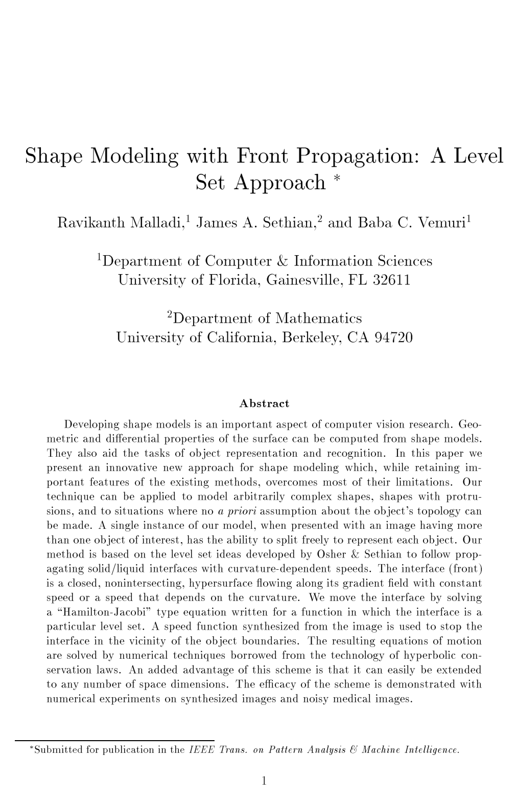
Shape Modeling with Front Propagation: A Level Set Approach

R. MalladiJames A. SethianBaba C. Vemuri

article1995TPAMI3,675 citations

Develops a level set framework for shape recovery that naturally handles topological changes like splitting and merging to reconstruct complex, branching structures from noisy images without relying on close initialization.

Listen

Researchers have long sought reliable ways to recover the shapes of objects from noisy two-dimensional images for applications such as medical analysis and object recognition. Existing techniques, including active-contour models, often require an initial guess close to the true boundary and assume a fixed object topology; as a result they fail on shapes with branches or protrusions and cannot split to represent multiple objects in one scene.

The work evaluates a new shape-recovery procedure that embeds the evolving boundary in a higher-dimensional function and advances it according to a speed derived from image gradients. The procedure solves the resulting equations with stable numerical schemes borrowed from conservation laws, allowing the front to stop automatically at object edges while handling arbitrary topology changes without user intervention.

Experiments on both synthetic images and real angiograms show that a single initial contour, placed anywhere inside the objects, converges to detailed boundaries regardless of starting position. The front successfully enters narrow protrusions, splits to isolate separate shapes, and produces consistent results on coarse as well as fine grids. In contrast, conventional active-contour models tested on the same arterial image either remain trapped or collapse to overly smooth outlines.

These capabilities remove the need for repeated manual initialization and topology specification, lowering the cost and time required for automated segmentation in noisy environments. The approach therefore supports downstream tasks such as quantitative measurement and motion tracking where shape accuracy directly affects diagnostic or operational decisions.

Further development should embed the algorithm in a multiresolution framework to reduce computation time on fine grids and should test extensions to three-dimensional medical volumes. The main remaining uncertainties concern performance on very sparse range data and the precise trade-off between grid resolution and boundary fidelity; additional controlled trials on diverse image types would strengthen before widespread deployment.

Cover for Shape Modeling with Front Propagation: A Level Set Approach

Abstract

Developing shape models is an important aspect of computer vision research. Geometric and differential properties of the surface can be computed from shape models. They also aid the tasks of object representation and recognition. In this paper we present an innovative new approach for shape modeling which, while retaining important features of the existing methods, overcomes most of their limitations. Our technique can be applied to model arbitrarily complex shapes, shapes with protrusions, and to situations where no a priori assumption about the object’s topology can be made. A single instance of our model, when presented with an image having more than one object of interest, has the ability to split freely to represent each object. Our method is based on the level set ideas developed by Osher & Sethian to follow propagating solid/liquid interfaces with curvature-dependent speeds. The interface (front) is a closed, nonintersecting, hypersurface flowing along its gradient field with constant speed or a speed that depends on the curvature. We move the interface by solving aHamilton-Jacobitype equation written for a function in which the interface is a particular level set. A speed function synthesized from the image is used to stop the interface in the vicinity of the object boundaries. The resulting equations of motion are solved by numerical techniques borrowed from the technology of hyperbolic conservation laws. An added advantage of this scheme is that it can easily be extended to any number of space dimensions. The efficacy of the scheme is demonstrated with numerical experiments on synthesized images and noisy medical images.

Table of Contents

  • 1 Introduction
  • 1.1 Overview
  • 2 Front propagation problem
  • 3 Shape reconstruction with front propagation
  • 4 Numerical solution and experimental results
  • 4.1 Experimental results
  • 5 Concluding remarks

Knowls

  1. Knowl 1 — Level Set Representation for Deformable Shape Modeling

    model/method

    Deformable boundary modeling is formulated by embedding a propagating (N1)(N-1)-dimensional interface (front) γ(t)\gamma(t) as the zero level set of a higher-dimensional time-dependent scalar function ψ(x,t):RN×[0,)R\psi(\mathbf{x}, t): \mathbb{R}^N \times [0, \infty) \to \mathbb{R}:

    γ(t)={xRNψ(x,t)=0}\gamma(t) = \{\mathbf{x} \in \mathbb{R}^N \mid \psi(\mathbf{x}, t) = 0\}

    At initial time t=0t = 0, ψ(x,0)\psi(\mathbf{x}, 0) is defined via the signed distance function:

    ψ(x,0)=±d(x)\psi(\mathbf{x}, 0) = \pm d(\mathbf{x})

    where d(x)d(\mathbf{x}) is the shortest Euclidean distance from point x\mathbf{x} to the initial interface γ(0)\gamma(0), taking a positive sign if x\mathbf{x} is outside the closed interface γ(0)\gamma(0) and a negative sign if inside.

    When every level set of ψ\psi propagates along its normal direction n=ψψ\mathbf{n} = \frac{\nabla \psi}{|\nabla \psi|} with scalar speed FF, differentiating the identity ψ(x(t),t)=0\psi(\mathbf{x}(t), t) = 0 with respect to time yields the Hamilton-Jacobi-type evolution equation:

    ψt+Fψ=0\psi_t + F |\nabla \psi| = 0

    Because the underlying coordinate grid remains fixed while the zero level set moves implicitly, the model handles topological transformations (splitting, merging, and pinching) and geometric singularities automatically without reparameterization or discrete marker bookkeeping.

  2. Knowl 2 — Curvature and Geometric Diffusion Term in 2D Level Sets

    equation

    When front propagation includes geometric regularization, the net speed FF is decomposed into an advection speed FAF_A and a geometry-dependent diffusion speed FG=ϵKF_G = -\epsilon K, where ϵ0\epsilon \ge 0 is a smoothing constant and KK is the local curvature of the level curve.

    For a two-dimensional domain x=(x,y)R2\mathbf{x} = (x, y) \in \mathbb{R}^2, the curvature KK at any point of the level set function ψ\psi is computed directly from its first and second spatial derivatives:

    K=(ψψ)=ψyyψx22ψxψyψxy+ψxxψy2(ψx2+ψy2)3/2K = \nabla \cdot \left( \frac{\nabla \psi}{|\nabla \psi|} \right) = \frac{\psi_{yy}\psi_x^2 - 2\psi_x \psi_y \psi_{xy} + \psi_{xx}\psi_y^2}{(\psi_x^2 + \psi_y^2)^{3/2}}

    Substituting F(K)=1ϵKF(K) = 1 - \epsilon K (or FAϵKF_A - \epsilon K) into the front propagation equation produces the viscous Hamilton-Jacobi formulation:

    ψt+ψ=ϵKψ\psi_t + |\nabla \psi| = \epsilon K |\nabla \psi|

    where the parabolic right-hand side acts as an intrinsic curvature-smoothing (viscous diffusion) term that prevents front instability and smooths high-curvature corners.

  3. Knowl 3 — Image-Synthesized Stopping Speeds for Front Arrest

    model/method

    To stop the evolving level set interface at target object boundaries in an intensity image I(x,y)I(x,y), image-dependent stopping functions are constructed from smoothed image gradients:

    1. Additive Stopping Term (Constant Speed / Pure Advection Case, F=FAF = F_A):

    FI(x,y)=FAM1M2(GσI(x,y)M2)F_I(x,y) = \frac{-F_A}{M_1 - M_2} \left( |\nabla G_\sigma * I(x,y)| - M_2 \right)

    where GσIG_\sigma * I denotes convolution of the image with a 2D Gaussian filter of standard deviation σ\sigma, and M1,M2M_1, M_2 are the maximum and minimum values of GσI(x,y)|\nabla G_\sigma * I(x,y)| across the image domain Ω\Omega. As image gradients increase toward M1M_1, FIF_I approaches FA-F_A, driving the total propagation speed FA+F^IF_A + \hat{F}_I to zero in the evolution equation:

    ψt+(FA+F^I)ψ=0\psi_t + (F_A + \hat{F}_I) |\nabla \psi| = 0

    1. Multiplicative Stopping Term (Curvature-Dependent Case, F=FA+FGF = F_A + F_G):

    kI(x,y)=11+GσI(x,y)k_I(x,y) = \frac{1}{1 + |\nabla G_\sigma * I(x,y)|}

    where kI(x,y)(0,1]k_I(x,y) \in (0, 1] scales the combined advection and geometric diffusion speeds, yielding the evolution equation:

    ψt+k^I(FA+FG)ψ=0\psi_t + \hat{k}_I (F_A + F_G) |\nabla \psi| = 0

    Here, F^I\hat{F}_I and k^I\hat{k}_I represent global extensions of the image terms off the zero level set.

  4. Knowl 4 — Speed Extension Off the Zero Level Set

    definition

    Because image-derived terms FI(x,y)F_I(x,y) and kI(x,y)k_I(x,y) are physically meaningful only along the target object boundary where the moving contour {ψ=0}\{\psi = 0\} is located, their values must be extended across the entire domain Ω\Omega to evolve all neighboring level sets {ψ=C}\{\psi = C\} without causing level sets to collide or cross each other.

    Extension Construction: The value of the extended speed function F^I\hat{F}_I (or k^I\hat{k}_I) at any point PP lying on the level set {ψ=C}\{\psi = C\} is defined as the value of FIF_I (or kIk_I) at the point QQ lying on the zero level set {ψ=0}\{\psi = 0\} that is at Euclidean distance C|C| from PP along the normal trajectory.

    This construction ensures that F^IFI\hat{F}_I \equiv F_I and k^IkI\hat{k}_I \equiv k_I on {ψ=0}\{\psi = 0\}, adheres to Huygens' principle, and prevents level curves from crossing during propagation.

  5. Knowl 5 — Entropy-Satisfying Upwind Numerical Scheme for Front Evolution

    algorithm

    To preserve sharp corners and select the correct entropy-satisfying weak solution without unphysical oscillations, spatial derivatives in the hyperbolic advective term are approximated using Osher-Sethian upwind finite differences, while the parabolic curvature term is approximated by central differences.

    Let ψi,jnψ(iΔx,jΔy,nΔt)\psi_{i,j}^n \approx \psi(i\Delta x, j\Delta y, n\Delta t) on a grid with spacing Δx=Δy=h\Delta x = \Delta y = h. Define standard difference operators:

    Dxψi,j=ψi,jnψi1,jnΔx,Dx+ψi,j=ψi+1,jnψi,jnΔxD_x^- \psi_{i,j} = \frac{\psi_{i,j}^n - \psi_{i-1,j}^n}{\Delta x}, \quad D_x^+ \psi_{i,j} = \frac{\psi_{i+1,j}^n - \psi_{i,j}^n}{\Delta x}

    Dyψi,j=ψi,jnψi,j1nΔy,Dy+ψi,j=ψi,j+1nψi,jnΔyD_y^- \psi_{i,j} = \frac{\psi_{i,j}^n - \psi_{i,j-1}^n}{\Delta y}, \quad D_y^+ \psi_{i,j} = \frac{\psi_{i,j+1}^n - \psi_{i,j}^n}{\Delta y}

    Input: Grid values ψi,jn\psi_{i,j}^n, extended image factor (k^I)i,j(\hat{k}_I)_{i,j}, advection speed FAF_A, curvature factor ϵ\epsilon, grid spacing hh, time step Δt\Delta t
    Output: Updated level set values ψi,jn+1\psi_{i,j}^{n+1}
    for each grid cell (i,j)(i,j) do
        x,upwind2max(Dxψi,jn,0)2+min(Dx+ψi,jn,0)2\nabla_{x,\text{upwind}}^2 \leftarrow \max(D_x^- \psi_{i,j}^n, 0)^2 + \min(D_x^+ \psi_{i,j}^n, 0)^2
        y,upwind2max(Dyψi,jn,0)2+min(Dy+ψi,jn,0)2\nabla_{y,\text{upwind}}^2 \leftarrow \max(D_y^- \psi_{i,j}^n, 0)^2 + \min(D_y^+ \psi_{i,j}^n, 0)^2
        Θi,jx,upwind2+y,upwind2\Theta_{i,j} \leftarrow \sqrt{\nabla_{x,\text{upwind}}^2 + \nabla_{y,\text{upwind}}^2}
        Compute curvature Ki,jK_{i,j} and magnitude ψi,j|\nabla \psi_{i,j}| using standard central differences
        FGϵKi,jF_G \leftarrow -\epsilon K_{i,j}
        ψi,jn+1ψi,jnΔtFA(k^I)i,jΘi,jΔtFG(k^I)i,jψi,j\psi_{i,j}^{n+1} \leftarrow \psi_{i,j}^n - \Delta t \, F_A (\hat{k}_I)_{i,j} \, \Theta_{i,j} - \Delta t \, F_G (\hat{k}_I)_{i,j} \, |\nabla \psi_{i,j}|
    end for
    return ψn+1\psi^{n+1}
  6. Knowl 6 — Piecewise Linear Extraction of Zero Level Contours

    algorithm

    To identify the instantaneous interface location γ(t)={xψ(x,t)=0}\gamma(t) = \{\mathbf{x} \mid \psi(\mathbf{x}, t) = 0\} for visualization and speed extension evaluation without explicit marker particle tracking:

    Input: 2D scalar field ψi,j\psi_{i,j} on Cartesian grid cells [i,i+1]×[j,j+1][i, i+1] \times [j, j+1]
    Output: List LL of line segments representing the zero level set contour
    Initialize LL \leftarrow \emptyset
    for each grid cell bounded by (i,j),(i+1,j),(i,j+1),(i+1,j+1)(i,j), (i+1,j), (i,j+1), (i+1,j+1) do
        vminmin(ψi,j,ψi+1,j,ψi,j+1,ψi+1,j+1)v_{\min} \leftarrow \min(\psi_{i,j}, \psi_{i+1,j}, \psi_{i,j+1}, \psi_{i+1,j+1})
        vmaxmax(ψi,j,ψi+1,j,ψi,j+1,ψi+1,j+1)v_{\max} \leftarrow \max(\psi_{i,j}, \psi_{i+1,j}, \psi_{i,j+1}, \psi_{i+1,j+1})
        if vmin0v_{\min} \le 0 and vmax0v_{\max} \ge 0 then
            Compute edge entrance point PenterP_{\text{enter}} where ψ=0\psi = 0 via 1D linear interpolation
            Compute edge exit point PexitP_{\text{exit}} where ψ=0\psi = 0 via 1D linear interpolation
            Append segment (Penter,Pexit)(P_{\text{enter}}, P_{\text{exit}}) to LL
        end if
    end for
    return LL
  7. Knowl 7 — Numerical Stability Conditions for Explicit Level Set Time Stepping

    theoretical result

    The numerical stability constraints for explicit time integration of the level set equation depend on whether curvature diffusion is present:

    1. Curvature-Dependent Diffusion (FG0F_G \neq 0): Because the curvature term introduces second-order spatial derivatives into the PDE, the explicit time step is subject to a parabolic stability restriction:

    Δt=O(Δx2)\Delta t = O(\Delta x^2)

    1. Pure Advection (FG=0F_G = 0): When the front propagates under constant normal speed without curvature regularization, the equation is a first-order hyperbolic Hamilton-Jacobi equation governed by the Courant-Friedrichs-Lewy (CFL) condition:

    Δt=O(Δx)\Delta t = O(\Delta x)

    To mitigate the computational cost of the small Δt\Delta t required by fine grids, the speed extension field k^I\hat{k}_I or F^I\hat{F}_I can be updated once every kk time steps (k>1k > 1) rather than at every integration step.

  8. Knowl 8 — Arterial Tree Segmentation and Protrusion Tracking

    empirical result

    In segmenting complex branching vasculature from digital subtraction angiograms:

    • Active Contour Model (Snakes with Balloon Forces): Across three distinct initializations of increasing proximity to the target vessel, the parametric active contour model fails to extract the branching arterial tree even after 1000 iterations. Due to internal energy minimization terms that penalize arc-length (elasticity) and curvature (rigidity), the snake snaps back into a smoothed, bumpless shape and cannot extrude into narrow vascular protrusions.
    • Level Set Front Propagation: Initialized as a simple closed curve within the vessel lumen, the level set front propagates along its normal vector field, enters narrow branches, and reconstructs the complete arterial tree in 391 iterations on a 64×6464 \times 64 grid with time step Δt=0.001\Delta t = 0.001. Shape recovery does not require placing the initialization near the boundary or optimizing a nonconvex objective functional.
  9. Knowl 9 — Dynamic Topological Splitting for Multi-Object Segmentation

    empirical result

    When a single initial closed curve is placed around an image containing three distinct disconnected objects and propagated inward in the negative normal direction:

    1. The zero level set {ψ=0}\{\psi = 0\} contracts, conforms around the outer boundaries of the three objects, and subsequently splits into four disconnected closed contours.
    2. Three of the closed contour segments wrap around and isolate the three individual target objects, while the fourth isolated segment formed in the void between the objects contracts to a point and disappears.
    3. Complete convergence to the three separate target boundaries is reached in 140 iterations on a 64×6464 \times 64 grid with Δt=0.001\Delta t = 0.001.

    This confirms that a single level set instance can dynamically change its topology and segment multiple disjoint objects simultaneously without explicit heuristics or split-and-merge algorithms.

  10. Knowl 10 — Fine-Grid Time Complexity and Sparse Data Reconstruction Limitations

    limitation

    The front propagation level set shape modeling framework has two main limitations:

    1. Parabolic Fine-Grid Time Step Restriction: The explicit stability requirement Δt=O(Δx2)\Delta t = O(\Delta x^2) severely restricts the allowable time step on high-resolution meshes (e.g., requiring Δt=0.00005\Delta t = 0.00005 on a 256×256256 \times 256 grid versus Δt=0.008\Delta t = 0.008 on a 64×6464 \times 64 grid), creating a substantial computational burden unless multiresolution coarse-to-fine acceleration is employed.
    2. Dependence on Dense Continuum Gradients: The stopping criteria rely on computing continuum image gradient fields across regular spatial grids. Consequently, the method cannot be directly applied in its continuous PDE form to reconstruct surface shapes from sparse, irregularly sampled range or depth data.

Coverage note — None was omitted; all primary contributions, mathematical equations, numerical algorithms, empirical findings, and stated limitations were fully extracted.

References

  1. 1.R. Bajcsy and S. Kovačič, “Multiresolution elastic matching,” Computer Vision, Graphics, and Image Processing, Vol. 46, pp. 1–21, 1989.
  2. 2.R. M. Bolle and B. C. Vemuri, “On three-dimensional surface reconstruction methods,” IEEE Trans. on Pattern Analysis and Machine Intelligence, vol. PAMI 13, No. 1, pp. 1–13, 1991.
  3. 3.T.E. Boult and J.R. Kender, “Visual surface reconstruction using sparse depth data,” in Proc. IEEE Conf. on Computer Vision and Pattern Recognition, June 1986, pp. 68–76.
  4. 4.A. Blake and A. Zisserman, Visual Reconstruction, MIT Press, Cambridge, MA.
  5. 5.L. D. Cohen, “On Active Contour Models and Balloons,” Computer Vision, Graphics, and Image Processing, Vol. 53, No. 2, pp. 211–218, March 1991.
  6. 6.L. D. Cohen and I. Cohen, “Deformable models for 3D medical images using finite elements and balloons,” in Proceedings of IEEE Conference on Computer Vision and Pattern Recognition, pp. , Urbana Illinois, June 1992.
  7. 7.H. Delingette, M. Hebert, and K. Ikeuchi, “Shape representation and image segmentation using deformable models,” in Proceedings of IEEE Conference on Computer Vision and Pattern Recognition, pp. 467–472, Maui Hawaii, June 1991.
  8. 8.L. C. Evans and J. Spruck, “Motion of level sets by mean curvature. I,” Journal of Differential Geometry, Vol. 33, pp. 635–681, 1991.
  9. 9.M. Kass, A. Witkin, and D. Terzopoulos, “Snakes: Active Contour Models,” International Journal of Computer Vision, pp. 321–331, 1988.
  10. 10.B. B. Kimia, A. R. Tannenbaum, and S. W. Zucker, “Shapes, shocks, and deformations I: The components of shape and reaction-diffusion space,” Technical Report LEMS-105, Division of Engineering, Brown University, June 1992.
  11. 11.D. Lee and T. Pavlidis, “One-dimensional regularization with discontinuities,” IEEE Trans. on Pattern Analysis and Machine Intelligence, vol. PAMI 10, pp. 822–829, 1986.
  12. 12.R. Malladi, J. A. Sethian, and B. C. Vemuri, “A topology-independent shape modeling scheme,” in Proceedings of SPIE Conference on Geometric Methods in Computer Vision II, San Diego, July 1993.
  13. 13.S. Osher and J. A. Sethian, “Fronts propagating with curvature dependent speed: Algorithms based on Hamilton-Jacobi formulation,” Journal of Computational Physics, Vol. 79, pp. 12-49, 1988.
  14. 14.W. Press, B. Flannery, S. Teukolsky, and W. Vetterling, Numerical Recipes in C, Cambridge University Press, Cambridge, 1988.
  15. 15.R. Samadani, “Changes in connectivity in active contour models,” Proceedings of the Workshop on Visual Motion, pp. 337–343, Irvine California, March 1989.
  16. 16.R. Samadani, “Adaptive snakes: control of damping and material parameters,” Proceedings of SPIE Conference on Geometric Methods in Computer Vision, Vol. 1570, pp. 202–213, San Diego California, July 1991.
  17. 17.L.L. Schumaker, “Fitting Surfaces to Scattered data,” in Approximation Theory II, G.G. Lorentz, C.K. Chui, and L.L. Schumaker, (eds.). New York: Academic Press, 1976, pp. 203–267.
  18. 18.J. A. Sethian, “Curvature and the evolution of fronts,” Commun. in Mathematical Physics, Vol. 101, pp. 487–499, 1985.
  19. 19.J. A. Sethian, “Numerical algorithms for propagating interfaces: Hamilton-Jacobi equations and conservation laws,” Journal of Differential Geometry, Vol. 31, pp. 131–161, 1990.
  20. 20.R. Szeliski and D. Tonnesen, “Surface modeling with oriented particle systems,” Computer Graphics SIGGRAPH, Vol. 26, No. 2, pp. 185–194, July 1992.
  21. 21.D. Terzopoulos, “Regularization of inverse visual problems involving discontinuities,” IEEE Trans. on Pattern Analysis and Machine Intelligence, Vol. PAMI 8, No. 2, pp. 413–424, 1986.
  22. 22.D. Terzopoulos, A. Witkin, and M. Kass, “Constraints on deformable models: Recovering 3D shape and nonrigid motion,” Artificial Intelligence, 36, pp. 91–123, 1988.
  23. 23.D. Terzopoulos, “The computation of visible surface representations,” IEEE Trans. on Pattern Analysis and Machine Intelligence, vol. PAMI 4, Vol. 10, pp. 417–438, 1988.
  24. 24.B. C. Vemuri, A. Mitiche, and J. K. Aggarwal, "Curvature-based representation of objects from range data," Int. Journal of Image and Vision Computing, 4, pp. 107–114, 1986.
  25. 25.B. C. Vemuri and R. Malladi, “Deformable models: Canonical parameters for surface representation and multiple view integration,” Proc. IEEE Conference on Computer Vision and Pattern Recognition, pp. 724–725, Maui Hawaii, June 1991.
  26. 26.B. C. Vemuri and R. Malladi, “Surface griding with intrinsic parameters,” Pattern Recognition Letters, Vol. 13, No. 11, pp. 805–812, November 1992.
  27. 27.B. C. Vemuri and R. Malladi, “Constructing intrinsic parameters with active models for invariant surface reconstruction,” IEEE Trans. on Pattern Analysis and Machine Intelligence, in press.
  28. 28.Y. F. Wang and J. F. Wang, “Surface reconstruction using deformable models with interior and boundary constraints,” in Proceedings of ICCV, pp. 300–303, Osaka, Japan, 1990.

Citation

MLA
Malladi, R., et al. “Shape Modeling with Front Propagation: A Level Set Approach”. IEEE Transactions on Pattern Analysis and Machine Intelligence, vol. 17, no. 2, 1995, pp. 158–75, https://doi.org/10.1109/34.368173.
APA
Malladi, R., Sethian, J. A., & Vemuri, B. C. (1995). Shape modeling with front propagation: a level set approach. IEEE Transactions on Pattern Analysis and Machine Intelligence, 17(2), 158–175. https://doi.org/10.1109/34.368173
Chicago
Malladi, R., J. A. Sethian, and B. C. Vemuri. 1995. “Shape Modeling with Front Propagation: A Level Set Approach”. IEEE Transactions on Pattern Analysis and Machine Intelligence 17 (2): 158–75. https://doi.org/10.1109/34.368173.
Harvard
Malladi, R., Sethian, J.A. and Vemuri, B.C. (1995) “Shape modeling with front propagation: a level set approach”, IEEE Transactions on Pattern Analysis and Machine Intelligence, 17(2), pp. 158–175. Available at: https://doi.org/10.1109/34.368173.
Vancouver
1. Malladi R, Sethian JA, Vemuri BC (1995) Shape modeling with front propagation: a level set approach. IEEE Transactions on Pattern Analysis and Machine Intelligence 17:158–175

BibTeX

@article{Malladi_1995, title={Shape modeling with front propagation: a level set approach}, volume={17}, ISSN={0162-8828}, url={http://dx.doi.org/10.1109/34.368173}, DOI={10.1109/34.368173}, number={2}, journal={IEEE Transactions on Pattern Analysis and Machine Intelligence}, publisher={Institute of Electrical and Electronics Engineers (IEEE)}, author={Malladi, R. and Sethian, J.A. and Vemuri, B.C.}, year={1995}, pages={158–175} }
Metadata:Crossref

Access the Paper

This paper is available from its original source. Click below to access the PDF.

Open PDF