Graph Neural Controlled Differential Equations for Traffic Forecasting

Jeongwhan ChoiHwangyong ChoiJeehyun HwangNoseong Park

article2022AAAI504 citations

Develops a unified spatio-temporal neural controlled differential equation framework that continuously models both spatial graph dynamics and temporal traffic patterns, significantly outperforming existing baselines across benchmark forecasting datasets.

Listen

Accurate traffic forecasting is essential for modern transportation planning, congestion management, and smart city infrastructure. However, predicting road conditions remains challenging because traffic patterns continuously fluctuate over time and across interconnected road networks. A major operational hurdle is that standard models struggle with real-world sensor data, which is frequently irregular or missing due to hardware failures and communication dropouts.

The article demonstrates the effectiveness of a novel framework called Spatio-Temporal Graph Neural Controlled Differential Equation (STG-NCDE) for forecasting traffic volumes and speeds. The main objective is to provide high-accuracy, continuous time-series forecasting across road networks while inherently maintaining robustness against missing or irregular sensor readings.

To evaluate this framework, the authors integrated two continuous differential equation models—one capturing temporal dynamics and the other processing spatial graph connections—into a unified architecture. They conducted extensive empirical testing across six real-world highway benchmark datasets from the California Performance of Transportation System (PeMS), comparing the model against 20 baseline approaches. The evaluation assessed standard multi-step prediction tasks as well as stress tests where 10% to 50% of sensor observations were randomly omitted to simulate real-world data loss.

The findings show that STG-NCDE consistently outperformed all 20 baseline methods across all six datasets and evaluation metrics. Overall, older baseline models exhibited error rates roughly 10% to 28% higher than STG-NCDE, with the closest competing advanced models still trailing in average accuracy. Ablation analyses revealed that combining both temporal and spatial continuous modeling is essential for peak performance, as the unified model converged faster and achieved lower overall error than either component in isolation. Crucially, in irregular traffic tests where up to half of the sensor data was removed, STG-NCDE maintained stable, reliable predictions without architectural modifications, whereas standard baselines could not process such irregular inputs.

These results demonstrate that treating traffic data as continuous paths significantly reduces prediction errors and mitigates operational risks associated with intermittent sensor blackouts. For transportation authorities and decision-makers, adopting continuous differential equation frameworks can improve real-time traffic routing, enhance network safety, and reduce the maintenance costs required for rigid data cleaning pipelines.

Organizations seeking to improve traffic management should consider piloting continuous spatio-temporal architectures in operational forecasting environments, particularly where sensor reliability is variable. Further work should explore deploying these models within live transportation control centers and extending the architecture to other spatio-temporal domains such as weather modeling and energy grid management.

Confidence in these findings is high given the breadth of the comparative evaluation across standard public benchmarks. However, stakeholders should note that the evaluation was conducted on fixed highway network topologies with predetermined prediction windows, meaning performance on rapidly shifting urban network graphs may require further validation.

Yonsei University difference equations ordinary differential equations Graph Neural Controlled Differential Equations traffic forecasting spatio-temporal forecasting

arXiv: 2112.03558

Paper: Diffusion Convolutional Recurrent Neural Network: Data-Driven Traffic Forecasting, Yaguang Li et al. (2017). This paper establishes the foundational spatio-temporal graph modeling paradigm for traffic forecasting by integrating graph convolutions with recurrent sequence architectures.
Paper: Spatio-temporal Graph Convolutional Neural Network: A Deep Learning Framework for Traffic Forecasting, Bing Yu et al. (2017). This work introduces the combination of spectral graph convolutions and temporal convolutions for traffic forecasting, defining the core problem setting and baselines advanced by STG-NCDE.
Paper: Graph WaveNet for Deep Spatial-Temporal Graph Modeling, Zonghan Wu et al. (2019). This paper introduces adaptive graph learning and temporal convolutions for spatial-temporal forecasting, serving as a primary baseline and conceptual predecessor to continuous spatial-temporal modeling.
Paper: Adaptive Graph Convolutional Recurrent Network for Traffic Forecasting, Lei Bai et al. (2020). This work develops adaptive graph convolutional recurrent networks for traffic forecasting, establishing key benchmark architectures that STG-NCDE directly compares against.
Paper: GMAN: A Graph Multi-Attention Network for Traffic Prediction, Chuanpan Zheng et al. (2019). This paper proposes graph multi-attention networks for multi-step traffic prediction, providing foundational attention mechanisms for dynamic spatial-temporal modeling in transportation networks.
Paper: T-GCN: A Temporal Graph Convolutional Network for Traffic Prediction, Ling Zhao et al. (2018). This work presents the standard coupling of graph convolutional networks and gated recurrent units for urban traffic forecasting that STG-NCDE aims to supersede.
Paper: Graph Neural Network for Traffic Forecasting: A Survey, Weiwei Jiang et al. (2021). This survey provides a comprehensive taxonomy of graph neural networks and spatio-temporal architectures applied across traffic forecasting benchmarks.

Paper: LargeST: A Benchmark Dataset for Large-Scale Traffic Forecasting, Xu Liu et al. (2023). This work introduces a multi-year, large-scale traffic forecasting benchmark that provides an extensive real-world testbed to evaluate the scalability and accuracy of spatio-temporal graph models like STG-NCDE.
Paper: GREAD: Graph Neural Reaction-Diffusion Networks, Jeongwhan Choi et al. (2023). This paper extends differential equation frameworks on graphs by modeling both reaction and diffusion dynamics, offering a complementary continuous-depth perspective to neural controlled differential equations.
Paper: Neural Stochastic PDEs: Resolution-Invariant Learning of Continuous Spatiotemporal Dynamics, Cristopher Salvi et al. (2022). This paper generalizes continuous spatio-temporal modeling from ordinary and controlled differential equations to resolution-invariant neural stochastic partial differential equations.

Cover for Graph Neural Controlled Differential Equations for Traffic Forecasting

Abstract

Traffic forecasting is one of the most popular spatio-temporal tasks in the field of machine learning. A prevalent approach in the field is to combine graph convolutional networks and recurrent neural networks for the spatio-temporal processing. There has been fierce competition and many novel methods have been proposed. In this paper, we present the method of spatio-temporal graph neural controlled differential equation (STG-NCDE). Neural controlled differential equations (NCDEs) are a breakthrough concept for processing sequential data. We extend the concept and design two NCDEs: one for the temporal processing and the other for the spatial processing. After that, we combine them into a single framework. We conduct experiments with 6 benchmark datasets and 20 baselines. STG-NCDE shows the best accuracy in all cases, outperforming all those 20 baselines by non-trivial margins.

Topics

difference equations ordinary differential equations

Keywords

Graph Neural Controlled Differential Equations traffic forecasting spatio-temporal forecasting spatial-temporal graph adaptive adjacency matrix graph convolution ODE solvers NCDE model time series forecasting traffic flow

Introduction
Related Work and Preliminaries
Neural Ordinary Differential Equations (NODEs)
Neural Controlled Differential Equations (NCDEs)
Traffic Forecasting
Proposed Method
Overall Design
Graph Neural Controlled Differential Equations
How to Train
Experiments
Datasets
Experimental Settings
Experimental Results
Ablation, Sensitivity, and Additional Studies
Conclusions
Acknowledgements
References

Knowls

Knowl 1 — Spatio-Temporal Graph Neural Controlled Differential Equation Framework
model/method
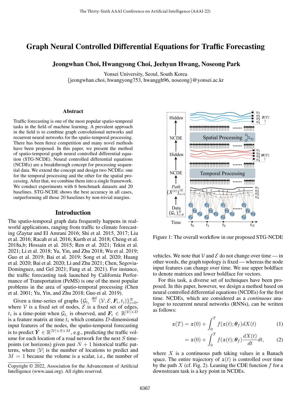
The Spatio-Temporal Graph Neural Controlled Differential Equation (STG-NCDE) framework processes time-series on static graphs $\mathcal{G} = (\mathcal{V}, \mathcal{E})$ with fixed node set $\mathcal{V}$ and edge set $\mathcal{E}$ . Let $\mathbf{X}(t) \in \mathbb{R}^{|\mathcal{V}| \times D}$ be a continuous multivariate path constructed from node feature time series over $t \in [0, T]$ .

STG-NCDE couples two neural controlled differential equations (NCDEs) sequentially:
1. Temporal NCDE: Computes node-wise continuous temporal representations $\mathbf{H}(t) \in \mathbb{R}^{|\mathcal{V}| \times \dim(\mathbf{h}^{(v)})}$ : $\mathbf{H}(T) = \mathbf{H}(0) + \int_0^T f(\mathbf{H}(t); \theta_f) \frac{d\mathbf{X}(t)}{dt} dt$ where $f: \mathbb{R}^{|\mathcal{V}| \times \dim(\mathbf{h}^{(v)})} \to \mathbb{R}^{|\mathcal{V}| \times \dim(\mathbf{h}^{(v)})}$ is a row-wise neural vector field parameterized by $\theta_f$ .
2. Spatial NCDE: Governs node spatial interaction states $\mathbf{Z}(t) \in \mathbb{R}^{|\mathcal{V}| \times \dim(\mathbf{z}^{(v)})}$ controlled by the temporal state trajectory $\mathbf{H}(t)$ : $\mathbf{Z}(T) = \mathbf{Z}(0) + \int_0^T g(\mathbf{Z}(t); \theta_g) \frac{d\mathbf{H}(t)}{dt} dt$ where $g: \mathbb{R}^{|\mathcal{V}| \times \dim(\mathbf{z}^{(v)})} \to \mathbb{R}^{|\mathcal{V}| \times \dim(\mathbf{z}^{(v)})}$ is a graph-convolutional vector field parameterized by $\theta_g$ .
Combining both stages yields a single Riemann-Stieltjes integral system: $\mathbf{Z}(T) = \mathbf{Z}(0) + \int_0^T g(\mathbf{Z}(t); \theta_g) f(\mathbf{H}(t); \theta_f) \frac{d\mathbf{X}(t)}{dt} dt$

For joint numerical integration, the system is formulated as an augmented ordinary differential equation (ODE): $\frac{d}{dt} \begin{bmatrix} \mathbf{Z}(t) \\ \mathbf{H}(t) \end{bmatrix} = \begin{bmatrix} g(\mathbf{Z}(t); \theta_g) f(\mathbf{H}(t); \theta_f) \frac{d\mathbf{X}(t)}{dt} \\ f(\mathbf{H}(t); \theta_f) \frac{d\mathbf{X}(t)}{dt} \end{bmatrix}$

The multi-step future traffic prediction $\hat{\mathbf{y}}^{(v)} \in \mathbb{R}^{S \times M}$ for node $v$ (across $S$ future horizons with $M$ feature dimensions) is generated from the final hidden state $\mathbf{z}^{(v)}(T)$ (the $v$ -th row of $\mathbf{Z}(T)$ ) via a linear output layer: $\hat{\mathbf{y}}^{(v)} = \mathbf{z}^{(v)}(T) \mathbf{W}_{\text{output}} + \mathbf{b}_{\text{output}}$ where $\mathbf{W}_{\text{output}} \in \mathbb{R}^{\dim(\mathbf{z}^{(v)}) \times (S \cdot M)}$ and $\mathbf{b}_{\text{output}} \in \mathbb{R}^{S \times M}$ .
Knowl 2 — Adaptive Spatial Graph CDE Vector Field
model/method
The spatial processing vector field $g(\mathbf{Z}(t); \theta_g) : \mathbb{R}^{|\mathcal{V}| \times \dim(\mathbf{z}^{(v)})} \to \mathbb{R}^{|\mathcal{V}| \times \dim(\mathbf{z}^{(v)})}$ in STG-NCDE integrates an adaptive graph convolution mechanism to mix representations across nodes $\mathcal{V}$ . It is defined as:

$\mathbf{B}_0 = \sigma(\text{FC}_{\dim(\mathbf{z}^{(v)}) \to \dim(\mathbf{z}^{(v)})}(\mathbf{Z}(t)))$ $\mathbf{B}_1 = \left(\mathbf{I} + \phi\left(\sigma\left(\mathbf{E} \cdot \mathbf{E}^T\right)\right)\right) \mathbf{B}_0 \mathbf{W}_{\text{spatial}}$ $g(\mathbf{Z}(t); \theta_g) = \psi(\text{FC}_{\dim(\mathbf{z}^{(v)}) \to \dim(\mathbf{z}^{(v)})}(\mathbf{B}_1))$

where:
- $\sigma$ is the ReLU activation function.
- $\psi$ is the hyperbolic tangent ( $\tanh$ ) activation function.
- $\text{FC}$ denotes a fully-connected layer applied row-wise.
- $\mathbf{I} \in \mathbb{R}^{|\mathcal{V}| \times |\mathcal{V}|}$ is the identity matrix.
- $\mathbf{E} \in \mathbb{R}^{|\mathcal{V}| \times C}$ is a learnable node-embedding matrix with embedding dimension $C$ , and $\mathbf{E}^T$ is its transpose.
- $\phi$ is the softmax function applied row-wise, normalizing the learned adaptive adjacency matrix $\mathbf{A} = \sigma(\mathbf{E} \cdot \mathbf{E}^T)$ .
- $\mathbf{W}_{\text{spatial}} \in \mathbb{R}^{\dim(\mathbf{z}^{(v)}) \times \dim(\mathbf{z}^{(v)})}$ is a learnable linear transformation weight matrix.
The operation $(\mathbf{I} + \phi(\sigma(\mathbf{E} \mathbf{E}^T)))\mathbf{B}_0 \mathbf{W}_{\text{spatial}}$ corresponds to a 1st-order Chebyshev polynomial graph convolution based on the normalized adaptive graph topology.
Knowl 3 — Temporal CDE Vector Field Parameterization
model/method
The temporal vector field $f(\mathbf{H}(t); \theta_f) : \mathbb{R}^{|\mathcal{V}| \times \dim(\mathbf{h}^{(v)})} \to \mathbb{R}^{|\mathcal{V}| \times \dim(\mathbf{h}^{(v)})}$ in STG-NCDE operates independently on each node's row representation in $\mathbf{H}(t)$ without cross-node mixing. It is parameterized as a $K$ -layer feedforward network:

$\mathbf{A}_0 = \sigma(\text{FC}_{\dim(\mathbf{h}^{(v)}) \to \dim(\mathbf{h}^{(v)})}(\mathbf{H}(t)))$ $\mathbf{A}_k = \sigma(\text{FC}_{\dim(\mathbf{h}^{(v)}) \to \dim(\mathbf{h}^{(v)})}(\mathbf{A}_{k-1})), \quad \text{for } k = 1, \dots, K-1$ $f(\mathbf{H}(t); \theta_f) = \psi(\text{FC}_{\dim(\mathbf{h}^{(v)}) \to \dim(\mathbf{h}^{(v)})}(\mathbf{A}_K))$

where $\sigma$ denotes the ReLU activation, $\psi$ denotes the hyperbolic tangent ( $\tanh$ ) activation, $\text{FC}$ denotes fully connected layers with weights in $\theta_f$ , and $K \in \{1, 2, 3\}$ is the depth of hidden transformations.
Knowl 4 — Continuous Path Construction and Initial Value Generation
model/method
Given discrete historical graph observations $\{\mathbf{G}_{t_i} = (\mathcal{V}, \mathcal{E}, \mathbf{F}_i, t_i)\}_{i=0}^N$ where $\mathbf{F}_i \in \mathbb{R}^{|\mathcal{V}| \times D}$ is the node feature matrix at time $t_i$ , STG-NCDE constructs a continuous-time representation before solving the differential equations:
1. Natural Cubic Spline Interpolation: For each node $v \in \mathcal{V}$ , the sequence of historical feature vectors $\{\mathbf{F}_i^{(v)}\}_{i=0}^N \subset \mathbb{R}^D$ is fitted using natural cubic splines to obtain a continuous, twice-differentiable trajectory $\mathbf{X}^{(v)}(t)$ over $t \in [0, T]$ , stacked as $\mathbf{X}(t) \in \mathbb{R}^{|\mathcal{V}| \times D}$ .
2. Initial State Mapping: The initial conditions $\mathbf{H}(0)$ and $\mathbf{Z}(0)$ are generated from the initial observation $\mathbf{F}_{t_0}$ via feedforward mappings: $\mathbf{H}(0) = \text{FC}_{D \to \dim(\mathbf{h}^{(v)})}(\mathbf{F}_{t_0})$ $\mathbf{Z}(0) = \text{FC}_{\dim(\mathbf{h}^{(v)}) \to \dim(\mathbf{z}^{(v)})}(\mathbf{H}(0))$
3. Training Objective: The parameters of the initial layers, CDE vector fields $f$ and $g$ , node embedding $\mathbf{E}$ , and output layer are optimized end-to-end using the $L_1$ loss over training set $\mathcal{T}$ : $\mathcal{L} = \frac{1}{|\mathcal{V}| \cdot |\mathcal{T}|} \sum_{\tau \in \mathcal{T}} \sum_{v \in \mathcal{V}} \|\mathbf{y}^{(\tau, v)} - \hat{\mathbf{y}}^{(\tau, v)}\|_1$ with $L_2$ weight decay regularization.
Knowl 5 — Well-Posedness of STG-NCDE Vector Fields
theoretical result
By the fundamental theory of controlled differential equations (Lyons, Caruana, and Lévy, 2007), an NCDE initial value problem is well-posed (i.e., a unique solution exists and depends continuously on the driving path) if the driving vector fields are Lipschitz continuous.

In STG-NCDE, the vector fields $f$ and $g$ are constructed entirely from standard neural network operations: linear fully connected layers, matrix multiplications with bounded parameter matrices, dropout, batch normalization, and standard activation functions (ReLU, Leaky ReLU, SoftPlus, Tanh, Sigmoid, Softmax), all of which have bounded Lipschitz constants (e.g., Lipschitz constant of 1 for ReLU and Tanh). Consequently, the composite vector fields $f(\mathbf{H}(t); \theta_f)$ and $g(\mathbf{Z}(t); \theta_g)$ satisfy Lipschitz continuity, ensuring that STG-NCDE defines a mathematically well-posed dynamical system with stable numerical training.
Knowl 6 — PeMS Traffic Forecasting Benchmark Setup
experimental setup
STG-NCDE is evaluated on six California Performance of Transportation System (PeMS) traffic benchmark datasets:
- PeMSD3: 358 nodes, 26,208 time steps (09/2018–11/2018), traffic volume (# of vehicles).
- PeMSD4: 307 nodes, 16,992 time steps (01/2018–02/2018), traffic volume.
- PeMSD7: 883 nodes, 28,224 time steps (05/2017–08/2017), traffic volume.
- PeMSD8: 170 nodes, 17,856 time steps (07/2016–08/2016), traffic volume.
- PeMSD7(M): 228 nodes, 12,672 time steps (05/2012–06/2012), traffic velocity.
- PeMSD7(L): 1,026 nodes, 12,672 time steps (05/2012–06/2012), traffic velocity.
Protocol:
- Sampling interval is 5 minutes.
- Datasets are split chronologically into training, validation, and test sets with a 6:2:2 ratio.
- Forecasting task: 12-sequence-to-12-sequence prediction ( $N=11$ past snapshots, $S=12$ future horizons, $M=1$ ).
- Evaluation metrics: Mean Absolute Error (MAE), Root Mean Squared Error (RMSE), and Mean Absolute Percentage Error (MAPE).
- Training hyperparameters: Adam optimizer, 200 epochs, batch size 64, hidden dimensions $\dim(\mathbf{h}^{(v)}), \dim(\mathbf{z}^{(v)}) \in \{32, 64, 128, 256\}$ , node embedding dimension $C \in \{1, \dots, 10\}$ , learning rate $\in \{10^{-4}, 5\times 10^{-4}, 10^{-3}, 5\times 10^{-3}, 10^{-2}\}$ , weight decay $\in \{10^{-4}, 10^{-3}, 10^{-2}\}$ , and early stopping patience of 15 epochs.

Knowl 7 — Traffic Volume Forecasting Performance Across PeMS Benchmarks

data/table

STG-NCDE outperforms competitive spatial-temporal deep learning baselines across all four traffic volume benchmarks (PeMSD3, PeMSD4, PeMSD7, PeMSD8) under the standard 12-to-12 prediction setting.

Model	PeMSD3			PeMSD4			PeMSD7			PeMSD8
	MAE	RMSE	MAPE	MAE	RMSE	MAPE	MAE	RMSE	MAPE	MAE	RMSE	MAPE
HA	31.58	52.39	33.78%	38.03	59.24	27.88%	45.12	65.64	24.51%	34.86	59.24	27.88%
ARIMA	35.41	47.59	33.78%	33.73	48.80	24.18%	38.17	59.27	19.46%	31.09	44.32	22.73%
VAR	23.65	38.26	24.51%	24.54	38.61	17.24%	50.22	75.63	32.22%	19.19	29.81	13.10%
FC-LSTM	21.33	35.11	23.33%	26.77	40.65	18.23%	29.98	45.94	13.20%	23.09	35.17	14.99%
TCN	19.32	33.55	19.93%	23.22	37.26	15.59%	32.72	42.23	14.26%	22.72	35.79	14.03%
GRU-ED	19.12	32.85	19.31%	23.68	39.27	16.44%	27.66	43.49	12.20%	22.00	36.22	13.33%
STGCN	17.55	30.42	17.34%	21.16	34.89	13.83%	25.33	39.34	11.21%	17.50	27.09	11.29%
DCRNN	17.99	30.31	18.34%	21.22	33.44	14.17%	25.22	38.61	11.82%	16.82	26.36	10.92%
GraphWaveNet	19.12	32.77	18.89%	24.89	39.66	17.29%	26.39	41.50	11.97%	18.28	30.05	12.15%
ASTGCN(r)	17.34	29.56	17.21%	22.93	35.22	16.56%	24.01	37.87	10.73%	18.25	28.06	11.64%
STSGCN	17.48	29.21	16.78%	21.19	33.65	13.90%	24.26	39.03	10.21%	17.13	26.80	10.96%
AGCRN	15.98	28.25	15.23%	19.83	32.26	12.97%	22.37	36.55	9.12%	15.95	25.22	10.09%
STFGNN	16.77	28.34	16.30%	20.48	32.51	16.77%	23.46	36.60	9.21%	16.94	26.25	10.60%
STGODE	16.50	27.84	16.69%	20.84	32.82	13.77%	22.59	37.54	10.14%	16.81	25.97	10.62%
Z-GCNETs	16.64	28.15	16.39%	19.50	31.61	12.78%	21.77	35.17	9.25%	15.76	25.11	10.01%
STG-NCDE	15.57	27.09	15.06%	19.21	31.09	12.76%	20.53	33.84	8.80%	15.45	24.81	9.92%

Across all six benchmark datasets, STG-NCDE achieves an overall average MAE of 12.72, RMSE of 21.33, and MAPE of 10.10%, outperforming the second-best baseline (Z-GCNETs at 13.22 MAE, 21.92 RMSE, 10.44% MAPE) and AGCRN (13.32 MAE, 22.29 RMSE, 10.37% MAPE).

Knowl 8 — Traffic Velocity Forecasting Performance on PeMSD7 Benchmarks

data/table

On the velocity forecasting benchmarks PeMSD7(M) and PeMSD7(L), STG-NCDE achieves lower prediction errors than existing spatial-temporal baseline models across MAE, RMSE, and MAPE.

Model	PeMSD7(M)			PeMSD7(L)
	MAE	RMSE	MAPE	MAE	RMSE	MAPE
HA	4.59	8.63	14.35%	4.84	9.03	14.90%
ARIMA	7.27	13.20	15.38%	7.51	12.39	15.83%
VAR	4.25	7.61	10.28%	4.45	8.09	11.62%
FC-LSTM	4.16	7.51	10.10%	4.66	8.20	11.69%
TCN	4.36	7.20	9.71%	4.05	7.29	10.43%
TCN(w/o causal)	4.43	7.53	9.44%	4.58	7.77	11.53%
GRU-ED	4.78	9.05	12.66%	3.98	7.71	10.22%
DSANet	3.52	6.98	8.78%	3.66	7.20	9.02%
STGCN	3.86	6.79	10.06%	3.89	6.83	10.09%
DCRNN	3.83	7.18	9.81%	4.33	8.33	11.41%
GraphWaveNet	3.19	6.24	8.02%	3.75	7.09	9.41%
ASTGCN(r)	3.14	6.18	8.12%	3.51	6.81	9.24%
MSTGCN	3.54	6.14	9.00%	3.58	6.43	9.01%
STG2Seq	3.48	6.51	8.95%	3.78	7.12	9.50%
LSGCN	3.05	5.98	7.62%	3.49	6.55	8.77%
STSGCN	3.01	5.93	7.55%	3.61	6.88	9.13%
AGCRN	2.79	5.54	7.02%	2.99	5.92	7.59%
STFGNN	2.90	5.79	7.23%	2.99	5.91	7.69%
STGODE	2.97	5.66	7.36%	3.22	5.98	7.94%
Z-GCNETs	2.75	5.62	6.89%	2.91	5.83	7.33%
STG-NCDE	2.68	5.39	6.76%	2.87	5.76	7.31%

Knowl 9 — Irregular Traffic Forecasting Robustness to Missing Sensor Observations

empirical result

Because STG-NCDE operates over continuous paths $\mathbf{X}(t)$ formed by natural cubic spline interpolation, it natively accommodates irregularly sampled or partially missing time-series without modifications to the neural architecture. Standard discrete graph neural networks cannot directly process irregular sequences.

Evaluating performance on PeMSD4 and PeMSD8 with randomly dropped sensor values (missing rates of 10%, 30%, and 50% applied independently per node) demonstrates minimal performance degradation for STG-NCDE:

Model	Missing	PeMSD4			PeMSD8
	Rate	MAE	RMSE	MAPE	MAE	RMSE	MAPE
STG-NCDE	10%	19.36	31.28	12.79%	15.68	24.96	10.05%
Only Temporal	10%	26.26	40.89	17.66%	21.18	33.02	13.26%
Only Spatial	10%	19.73	31.67	13.20%	16.85	26.63	11.12%
STG-NCDE	30%	19.40	31.30	13.04%	16.21	25.64	10.43%
Only Temporal	30%	26.86	41.73	18.35%	21.46	33.37	13.57%
Only Spatial	30%	19.83	31.95	13.29%	18.46	29.03	12.16%
STG-NCDE	50%	19.98	32.09	13.48%	16.68	26.17	10.67%
Only Temporal	50%	28.15	43.54	19.14%	22.68	35.14	14.11%
Only Spatial	50%	20.14	32.30	13.30%	17.98	28.12	11.87%

Even with 50% missing values on PeMSD4, STG-NCDE maintains an MAE of 19.98, compared to 19.21 on complete data.

Knowl 10 — Ablation Analysis of Spatial and Temporal NCDE Components
empirical result
To analyze the contribution of each NCDE component, two ablation variants are evaluated:
1. Only Temporal: Employs solely the temporal NCDE $\mathbf{H}(T) = \mathbf{H}(0) + \int_0^T f(\mathbf{H}(t); \theta_f) \frac{d\mathbf{X}(t)}{dt} dt$ , omitting spatial graph convolution.
2. Only Spatial: Employs solely the spatial NCDE directly driven by the input path $\mathbf{X}(t)$ , defined by: $\mathbf{Z}(T) = \mathbf{Z}(0) + \int_0^T g(\mathbf{Z}(t); \theta_g) \frac{d\mathbf{X}(t)}{dt} dt$
Experimental results show:
- On all datasets, the spatial-only model significantly outperforms the temporal-only model (e.g., PeMSD3 RMSE of 27.17 for spatial vs. 32.82 for temporal; PeMSD7 RMSE of 34.73 vs. 44.39).
- The full STG-NCDE combining both temporal and spatial NCDEs achieves superior accuracy over both variants (e.g., PeMSD3 RMSE of 27.09; PeMSD7 RMSE of 33.84).
- The training loss of the full STG-NCDE stabilizes after 2 epochs, whereas both ablation models take significantly longer to stabilize.
- Error metrics (MAE and MAPE) monotonically improve with node embedding dimension $C$ up to $C=7$ and achieve the best accuracy at $C=10$ .

Coverage note — Omitted specific qualitative node prediction plots and routine baseline descriptions, as their key empirical trends and performance numbers are fully captured in the benchmark and ablation knowls.

References

1.Bai, L.; Yao, L.; Kanhere, S. S.; Wang, X.; and Sheng, Q. Z. 2019. STG2Seq: Spatial-Temporal Graph to Sequence Model for Multi-step Passenger Demand Forecasting. In IJCAI.
2.Bai, L.; Yao, L.; Li, C.; Wang, X.; and Wang, C. 2020. Adaptive Graph Convolutional Recurrent Network for Traffic Forecasting. In NeurIPS, volume 33, 17804–17815.
3.Bai, S.; Kolter, J. Z.; and Koltun, V. 2018. An Empirical Evaluation of Generic Convolutional and Recurrent Networks for Sequence Modeling. arXiv:1803.01271.
4.Chen, C.; Petty, K.; Skabardonis, A.; Varaiya, P.; and Jia, Z. 2001. Freeway performance measurement system: mining loop detector data. Transportation Research Record, 1748(1): 96–102.
5.Chen, Y.; Segovia-Dominguez, I.; and Gel, Y. R. 2021. Z-GCNETs: Time Zigzags at Graph Convolutional Networks for Time Series Forecasting. In ICML.
6.Cheng, L.; Zang, H.; Ding, T.; Sun, R.; Wang, M.; Wei, Z.; and Sun, G. 2018a. Ensemble recurrent neural network based probabilistic wind speed forecasting approach. Energies, 11(8).
7.Cheng, W.; Shen, Y.; Zhu, Y.; and Huang, L. 2018b. A neural attention model for urban air quality inference: Learning the weights of monitoring stations. In AAAI.
8.Cho, K.; van Merrienboer, B.; Gulcehre, C.; Bougares, F.; Schwenk, H.; and Bengio, Y. 2014. Learning phrase representations using RNN encoder-decoder for statistical machine translation. In EMNLP.
9.Choi, J.; Choi, H.; Hwang, J.; and Park, N. 2021. Graph Neural Controlled Differential Equations for Traffic Forecasting. arXiv preprint arXiv:2112.03558.
10.Dormand, J.; and Prince, P. 1980. A family of embedded Runge-Kutta formulae. Journal of Computational and Applied Mathematics, 6(1): 19 – 26.
11.Fang, Z.; Long, Q.; Song, G.; and Xie, K. 2021. Spatial-Temporal Graph ODE Networks for Traffic Flow Forecasting. In KDD.
12.Guo, S.; Lin, Y.; Feng, N.; Song, C.; and Wan, H. 2019. Attention Based Spatial-Temporal Graph Convolutional Networks for Traffic Flow Forecasting. In AAAI.
13.Hamilton, J. D. 2020. Time series analysis. Princeton university press.
14.Hossain, M.; Rekabdar, B.; Louis, S. J.; and Dascalu, S. 2015. Forecasting the weather of Nevada: A deep learning approach. In IJCNN.
15.Huang, R.; Huang, C.; Liu, Y.; Dai, G.; and Kong, W. 2020. LSGCN: Long Short-Term Traffic Prediction with Graph Convolutional Networks. In IJCAI, 2355–2361.
16.Huang, S.; Wang, D.; Wu, X.; and Tang, A. 2019. DSANet: Dual Self-Attention Network for Multivariate Time Series Forecasting. In CIKM.
17.Kipf, T. N.; and Welling, M. 2017. Semi-Supervised Classification with Graph Convolutional Networks. In ICLR.
18.Kurth, T.; Treichler, S.; Romero, J.; Mudigonda, M.; Luehr, N.; Phillips, E.; Mahesh, A.; Matheson, M.; Deslippe, J.; Fatica, M.; et al. 2018. Exascale deep learning for climate analytics. In International Conference for High Performance Computing, Networking, Storage and Analysis. IEEE.
19.Li, M.; and Zhu, Z. 2021. Spatial-Temporal Fusion Graph Neural Networks for Traffic Flow Forecasting. In AAAI.
20.Li, Y.; Yu, R.; Shahabi, C.; and Liu, Y. 2018. Diffusion Convolutional Recurrent Neural Network: Data-Driven Traffic Forecasting. In ICLR.
21.Liu, Y.; Racah, E.; Correa, J.; Khosrowshahi, A.; Lavers, D.; Kunkel, K.; Wehner, M.; Collins, W.; et al. 2016. Application of deep convolutional neural networks for detecting extreme weather in climate datasets. arXiv preprint.
22.Lyons, T. J.; Caruana, M.; and Levy, T. 2007. Differential equations driven by rough paths. Springer.
23.Racah, E.; Beckham, C.; Maharaj, T.; Kahou, S. E.; Pal, C.; et al. 2016. ExtremeWeather: A large-scale climate dataset for semi-supervised detection, localization, and understanding of extreme weather events. arXiv preprint.
24.Ren, X.; Li, X.; Ren, K.; Song, J.; Xu, Z.; Deng, K.; and Wang, X. 2021. Deep Learning-Based Weather Prediction: A Survey. Big Data Research, 23.
25.Shi, X.; Chen, Z.; Wang, H.; Yeung, D.-Y.; Wong, W.-K.; and Woo, W.-c. 2015. Convolutional LSTM network: A machine learning approach for precipitation nowcasting. In NeurIPS.
26.Shi, X.; Gao, Z.; Lausen, L.; Wang, H.; Yeung, D.-Y.; Wong, W.-k.; and Woo, W.-c. 2017. Deep learning for precipitation nowcasting: A benchmark and a new model. arXiv preprint.
27.Song, C.; Lin, Y.; Guo, S.; and Wan, H. 2020. Spatial-Temporal Synchronous Graph Convolutional Networks: A New Framework for Spatial-Temporal Network Data Forecasting. In AAAI.
28.Sutskever, I.; Vinyals, O.; and Le, Q. V. 2014. Sequence to sequence learning with neural networks. In NeurIPS.
29.Tekin, S. F.; Karaahmetoglu, O.; Ilhan, F.; Balaban, I.; and Kozat, S. S. 2021. Spatio-temporal Weather Forecasting and Attention Mechanism on Convolutional LSTMs. arXiv preprint.
30.Wu, Z.; Pan, S.; Long, G.; Jiang, J.; and Zhang, C. 2019. Graph WaveNet for Deep Spatial-Temporal Graph Modeling. In IJCAI, 1907–1913.
31.Yu, B.; Yin, H.; and Zhu, Z. 2018. Spatio-Temporal Graph Convolutional Networks: A Deep Learning Framework for Traffic Forecasting. In IJCAI.
32.Zaytar, M. A.; and El Amrani, C. 2016. Sequence to sequence weather forecasting with long short-term memory recurrent neural networks. International Journal of Computer Applications.

Citation

MLA

Choi, J., et al. “Graph Neural Controlled Differential Equations for Traffic Forecasting”. arXiv, 2021, http://arxiv.org/abs/2112.03558v1.

APA

Choi, J., Choi, H., Hwang, J., & Park, N. (2021). Graph Neural Controlled Differential Equations for Traffic Forecasting. arXiv. http://arxiv.org/abs/2112.03558v1

Chicago

Choi, J., H. Choi, J. Hwang, and N. Park. 2021. “Graph Neural Controlled Differential Equations for Traffic Forecasting”. arXiv. http://arxiv.org/abs/2112.03558v1.

Harvard

Choi, J. et al. (2021) “Graph Neural Controlled Differential Equations for Traffic Forecasting”, arXiv [Preprint]. Available at: http://arxiv.org/abs/2112.03558v1.

Vancouver

1. Choi J, Choi H, Hwang J, Park N (2021) Graph Neural Controlled Differential Equations for Traffic Forecasting. arXiv

BibTeX

@article{choi2021graph,
  title = {Graph Neural Controlled Differential Equations for Traffic Forecasting},
  author = {Choi, Jeongwhan and Choi, Hwangyong and Hwang, Jeehyun and Park, Noseong},
  year = {2021},
  journal = {arXiv},
  url = {http://arxiv.org/abs/2112.03558v1},
  eprint = {2112.03558}
}

Metadata:arXiv

Access the Paper

This paper is available from its original source. Click below to access the PDF.

Open PDF

Graph Neural Controlled Differential Equations for Traffic Forecasting

Abstract

Topics

Keywords

Table of Contents

Knowls

Knowl 1 — Spatio-Temporal Graph Neural Controlled Differential Equation Framework

Knowl 2 — Adaptive Spatial Graph CDE Vector Field

Knowl 3 — Temporal CDE Vector Field Parameterization

Knowl 4 — Continuous Path Construction and Initial Value Generation

Knowl 5 — Well-Posedness of STG-NCDE Vector Fields

Knowl 6 — PeMS Traffic Forecasting Benchmark Setup