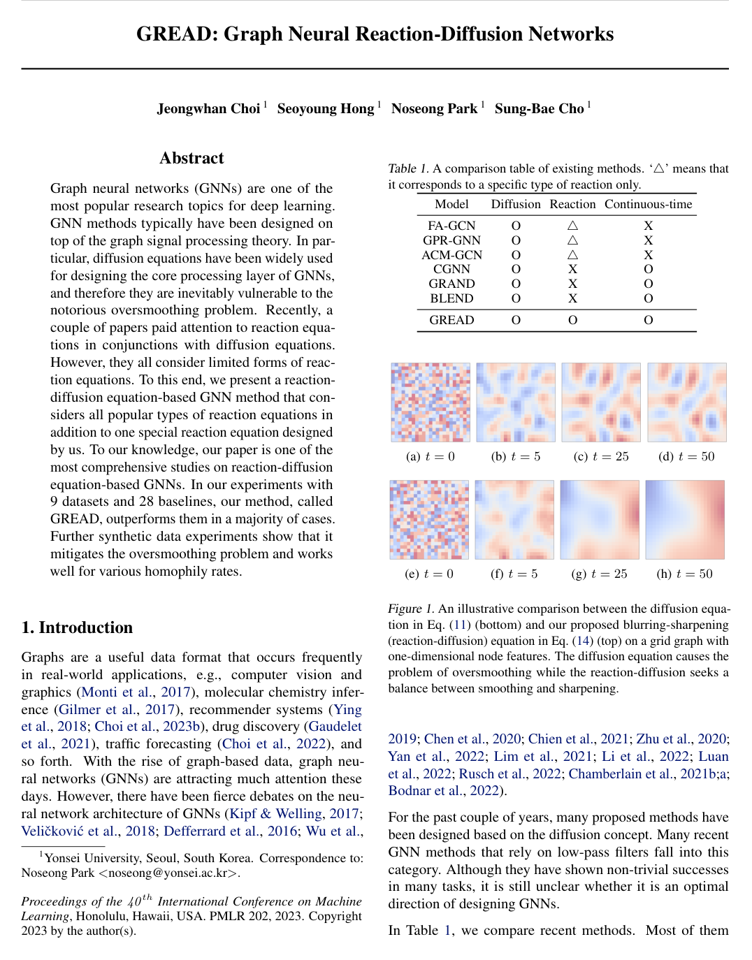
GREAD: Graph Neural Reaction-Diffusion Networks

Jeongwhan ChoiSeoyoung HongNoseong ParkSung-Bae Cho

article2023ICML59 citations

Develops a continuous graph neural network framework based on reaction-diffusion equations that incorporates diverse reaction mechanisms to effectively overcome the oversmoothing problem across both homophilic and heterophilic graphs.

Listen

Graph neural networks are widely used in machine learning for applications ranging from recommender systems to molecular chemistry. However, prevailing models rely heavily on diffusion equations (low-pass filtering) that cause oversmoothing, where node features converge to uniform values as network depth increases. Additionally, standard models struggle on heterophilic graphs, where interconnected nodes possess different labels rather than similar ones.

The article evaluates Graph Neural Reaction-Diffusion Networks (GREAD), a continuous-time framework designed to overcome these fundamental limitations. The primary objective is to demonstrate that integrating diverse reaction processes with diffusion prevents feature oversmoothing and delivers superior classification performance across diverse network structures.

The authors conducted a comprehensive empirical evaluation comparing GREAD against 28 baseline architectures across nine real-world datasets spanning high and low homophily, alongside controlled synthetic experiments. The framework incorporates seven distinct reaction formulations, including classical scientific formulations and an author-designed blurring-sharpening mechanism, solved continuously using neural ordinary differential equation solvers and an optional learned soft adjacency matrix.

The core findings indicate that GREAD-BS (the blurring-sharpening variant) achieves the highest overall performance, securing an average rank of 1.56 and 76.64% mean accuracy across real-world datasets, outperforming leading baselines like GloGNN (74.99%) and ACM-GCN (74.92%) with statistical significance. In synthetic stress tests, GREAD maintained stable classification across all homophily levels, whereas pure-diffusion models suffered sharp performance degradations. Energy tracking confirmed that traditional models lost expressive diversity within five layers, while GREAD bounded feature energy over 40 layers, successfully avoiding oversmoothing.

These results demonstrate that reaction-diffusion dynamics provide a robust architectural foundation for enterprise graph analytics. By dynamically balancing smoothing with sharpening, organizations can deploy deeper, more reliable graph models across heterogeneous relational data without incurring failure modes typical of pure diffusion-based approaches.

Organizations developing graph-based machine learning systems should consider adopting reaction-diffusion layers, particularly the blurring-sharpening variant paired with learned soft adjacency matrices and vector parameters, when handling complex or heterophilic network data. While GREAD introduces minor computational overhead due to additional reaction calculations and lacks global Lipschitz continuity under soft adjacency configurations, its consistent empirical gains provide high confidence in its operational effectiveness.

Yonsei University deep learning diffusion equations graph neural networks Graph Neural Reaction-Diffusion Networks GREAD reaction-diffusion layer

arXiv: 2211.14208

Paper: Neural Sheaf Diffusion: A Topological Perspective on Heterophily and Oversmoothing in GNNs, Cristian Bodnar et al. (2022). Provides the foundational continuous-time and geometric perspective on treating oversmoothing and heterophily via generalized differential diffusion operators on graphs.
Paper: Graph-Coupled Oscillator Networks, T. Konstantin Rusch et al. (2022). Introduces continuous physical dynamical systems (coupled oscillators) to prevent oversmoothing and gradient degradation in deep graph neural architectures.
Paper: Measuring and Relieving the Over-smoothing Problem for Graph Neural Networks from the Topological View, Deli Chen et al. (2019). Establishes standard topological metrics and conceptual analysis of the oversmoothing phenomenon in graph neural networks.
Paper: Beyond Homophily in Graph Neural Networks: Current Limitations and Effective Designs, Jiong Zhu et al. (2020). Analyzes the foundational limitations of standard GNNs under heterophily and outlines essential structural design principles for non-homophilous graphs.
Paper: Finding Global Homophily in Graph Neural Networks When Meeting Heterophily, Xiang Li et al. (2022). Introduces GloGNN, a key competitive baseline benchmarked against GREAD for learning representations across heterophilic graphs.
Paper: Simple and Deep Graph Convolutional Networks, Ming Chen et al. (2020). Demonstrates early architectural methods for maintaining expressive diversity and preventing oversmoothing in deep graph networks.
Paper: Geom-GCN: Geometric Graph Convolutional Networks, Hongbin Pei et al. (2020). Presents geometric approaches and continuous embedding spaces to tackle structural bottlenecks on disassortative and heterophilic graphs.
Paper: Diffusion-Convolutional Neural Networks, James Atwood et al. (2015). Introduces diffusion processes as a foundational message-passing mechanism on graph-structured data.

Paper: Characterizing Graph Datasets for Node Classification: Homophily-Heterophily Dichotomy and Beyond, Oleg Platonov et al. (2023). Extends the evaluation of heterophily by establishing formal informativeness metrics to reassess the performance and benchmarks of models designed for non-homophilous graphs.
Paper: Demystifying Structural Disparity in Graph Neural Networks: Can One Size Fit All?, Haitao Mao et al. (2023). Investigates local structural disparity between homophilic and heterophilic nodes within the same graph, offering deeper theoretical error bounds for non-uniform graph architectures.
Paper: Ordered GNN: Ordering Message Passing to Deal with Heterophily and Over-smoothing, Yunchong Song et al. (2023). Presents an alternative architectural strategy for simultaneously mitigating oversmoothing and heterophily via neuron-level hierarchical gating.
Paper: On Over-Squashing in Message Passing Neural Networks: The Impact of Width, Depth, and Topology, Francesco Di Giovanni et al. (2023). Provides formal sensitivity bounds connecting continuous and deep graph propagation to topological over-squashing and effective resistance.

Cover for GREAD: Graph Neural Reaction-Diffusion Networks

Abstract

Graph neural networks (GNNs) are one of the most popular research topics for deep learning. GNN methods typically have been designed on top of the graph signal processing theory. In particular, diffusion equations have been widely used for designing the core processing layer of GNNs, and therefore they are inevitably vulnerable to the notorious oversmoothing problem. Recently, a couple of papers paid attention to reaction equations in conjunctions with diffusion equations. However, they all consider limited forms of reaction equations. To this end, we present a reaction-diffusion equation-based GNN method that considers all popular types of reaction equations in addition to one special reaction equation designed by us. To our knowledge, our paper is one of the most comprehensive studies on reaction-diffusion equation-based GNNs. In our experiments with 9 datasets and 28 baselines, our method, called GREAD, outperforms them in a majority of cases. Further synthetic data experiments show that it mitigates the oversmoothing problem and works well for various homophily rates.

1. Introduction
2. Preliminaries & Related Work
2.1. Reaction-Diffusion Equations
2.2. Graph Neural Networks
2.3. Neural Ordinary Differential Equations (NODEs)
3. Proposed Method
3.1. Overview of GREAD
3.2. Soft Adjacency Matrix Generation
3.3. Reaction-diffusion Layer
3.4. Training Algorithm
3.5. Comparison with GNNs
4. Experiments
4.1. Node Classification on Real-world Datasets
4.2. Oversmoothing and Dirichlet Energy
4.3. Different Homophily Levels
5. Conclusions
Acknowledgement
References
A. Full Ranking of Table 2
B. Full Result of Table 4
C. Full Derivation of Eq. (12)
D. Computational Complexity
E. Additional Details for Experiments
E.1. Details of Datasets
E.2. Details of Experimental Settings
F. Additional Experimental Results on Real-world Datasets
F.1. Ablation Studies
F.2. Sensitivity Analyses
F.3. Training Time
F.4. Visualizations
G. Additional Experimental Results on Synthetic Datasets
G.1. Ablation Studies on β
H. Comparison with GRAND++ and GREAD-ST
I. Well-posedness of GREAD
J. Statistical Testing on Cora Dataset

Knowls

Knowl 1 — Continuous Graph Neural Reaction-Diffusion Architecture
model/method
The Graph Neural Reaction-Diffusion Network (GREAD) models feature propagation over a graph $\mathcal{G} = (\mathcal{V}, \mathcal{E})$ as a continuous dynamical system governed by a reaction-diffusion ordinary differential equation (ODE).

Let $X \in \mathbb{R}^{|\mathcal{V}| \times F}$ be the input node feature matrix for $|\mathcal{V}|$ nodes with $F$ features, and let $\tilde{L} = I - \tilde{A}$ denote the normalized graph Laplacian, where $\tilde{A} \in [0, 1]^{|\mathcal{V}| \times |\mathcal{V}|}$ is either the standard symmetric normalized adjacency matrix $A = D^{-1/2} A^{\text{raw}} D^{-1/2}$ or a parameterized soft adjacency matrix. The GREAD model consists of three sequential components:
1. Encoding Layer: $H(0) = e(X)$ where $e: \mathbb{R}^{|\mathcal{V}| \times F} \to \mathbb{R}^{|\mathcal{V}| \times d}$ is an encoder composed of fully-connected layers with Rectified Linear Unit (ReLU) activations.
2. Reaction-Diffusion Layer: $H(T) = H(0) + \int_0^T f(H(t)) \, dt$ where $T > 0$ is the terminal integration time, solved using numerical ODE solvers (such as Euler, 4th-order Runge-Kutta (RK4), or Dormand-Prince (DOPRI5)), and the vector field $f(H(t)) := \frac{dH(t)}{dt}$ is defined as: $f(H(t)) = -\alpha \tilde{L} H(t) + \beta r(H(t))$ Here, $-\alpha \tilde{L} H(t)$ is the diffusion term (low-pass smoothing operator), $r(H(t))$ is a reaction term, $\alpha$ is a trainable diffusion weighting parameter, and $\beta$ is a trainable reaction weighting parameter. Both $\alpha$ and $\beta$ can be configured as shared scalar coefficients (SC) or node-wise learnable vector coefficients (VC) of dimension $|\mathcal{V}|$ .
3. Output Layer: $\hat{y} = o(H(T))$ where $o: \mathbb{R}^{|\mathcal{V}| \times d} \to \mathbb{R}^{|\mathcal{V}| \times C}$ is a fully-connected classification layer followed by a softmax activation across $C$ target classes.
Knowl 2 — Reaction Terms in Graph Neural Reaction-Diffusion Networks
equation
In the GREAD reaction-diffusion layer, the reaction term $r(H(t)) \in \mathbb{R}^{|\mathcal{V}| \times d}$ controls local transformation and feature sharpening to balance global diffusion. The framework defines seven distinct reaction formulations:

$r(H(t)) := \begin{cases} H(t) \odot (1 - H(t)), & \text{if Fisher (F)} \\ H(t) \odot (1 - H(t)^{\circ 2}), & \text{if Allen-Cahn (AC)} \\ H(t) \odot (H(t) - H(t)^{\circ 2}), & \text{if Zeldovich (Z)} \\ (\tilde{A} - \tilde{A}^2) H(t), & \text{if Blurring-Sharpening (BS)} \\ H(0), & \text{if Source Term (ST)} \\ \tilde{L} H(t), & \text{if Filter Bank (FB)} \\ \tilde{L} H(t) + H(t), & \text{if Filter Bank* (FB*)} \end{cases}$

where $\odot$ denotes the element-wise Hadamard product, $H(t)^{\circ 2} = H(t) \odot H(t)$ is the Hadamard square, $\tilde{A}$ is the normalized (or soft) adjacency matrix, $\tilde{L} = I - \tilde{A}$ is the corresponding graph Laplacian, and $H(0)$ is the initial node embedding representation.

The Fisher, Allen-Cahn, and Zeldovich terms represent classical nonlinear reaction equations from population biology, phase separation alloy systems, and combustion theory, respectively. The Filter Bank variants (FB and FB*) inject explicit high-pass graph filtering signals and identity shortcuts into the velocity vector field.
Knowl 3 — Blurring-Sharpening Reaction-Diffusion Formulation
model/method
The Blurring-Sharpening (BS) reaction dynamics is derived by alternating low-pass smoothing (blurring) and high-pass sharpening graph filtering operations within an infinitesimal step $h$ .

Given the current node representation $H(t)$ and normalized adjacency $\tilde{A}$ with Laplacian $\tilde{L} = I - \tilde{A}$ , the blurring step produces an intermediate state: $B(t + h) = H(t) - \tilde{L}H(t) = \tilde{A} H(t)$

Applying a high-pass sharpening operation to $B(t + h)$ yields: $H(t + h) = B(t + h) + \tilde{L}(B(t + h)) = \tilde{A} H(t) + (I - \tilde{A}) \tilde{A} H(t) = (2I - \tilde{A}) \tilde{A} H(t)$

Rewriting $(2I - \tilde{A})\tilde{A}$ in terms of the Laplacian and adjacency matrices gives: $H(t + h) = H(t) - \tilde{L}H(t) + (\tilde{A} - \tilde{A}^2)H(t)$

Forming the finite difference $\frac{H(t + h) - H(t)}{h}$ and taking the continuous limit $h \to 0$ with learnable scaling coefficients $\alpha$ and $\beta$ yields the differential equation: $\frac{dH(t)}{dt} = -\alpha \tilde{L} H(t) + \beta (\tilde{A} - \tilde{A}^2) H(t)$

This demonstrates that alternating discrete low-pass and high-pass graph convolutions reduces to a continuous reaction-diffusion equation where the reaction function is specifically $r(H(t)) = (\tilde{A} - \tilde{A}^2) H(t)$ .
Knowl 4 — Soft Adjacency Matrix Generation via Scaled Dot-Product Attention
model/method
To learn dynamic, feature-dependent diffusivity across graph nodes, GREAD parameterizes a soft adjacency matrix $\tilde{A} \in [0, 1]^{|\mathcal{V}| \times |\mathcal{V}|}$ using scaled dot-product attention over node representations.

For any pair of nodes $i, j \in \mathcal{V}$ with embedding vectors $H_i, H_j \in \mathbb{R}^d$ , the soft adjacency matrix element $\tilde{A}_{[i,j]}$ is computed as: $\tilde{A}_{[i,j]} := \text{softmax}_j \left( \frac{(W_K H_i)^T (W_Q H_j)}{d_K} \right)$ where $W_K, W_Q \in \mathbb{R}^{d_K \times d}$ are learnable projection matrices, and $d_K$ is the scaling dimensionality factor. The corresponding soft Laplacian matrix is computed as $\tilde{L} = I - \tilde{A}$ , which replaces the static normalized Laplacian in the diffusion and reaction operations to allow adaptive spatial propagation.
Knowl 5 — Oversmoothing Mitigation and Dirichlet Energy Conservation
theoretical result
The degree of oversmoothing in deep graph neural networks is quantified by the Dirichlet energy $E(H, A^{\text{raw}})$ of node representations $H \in \mathbb{R}^{|\mathcal{V}| \times d}$ on an undirected graph $\mathcal{G} = (\mathcal{V}, \mathcal{E})$ with adjacency $A^{\text{raw}}$ :

$E(H, A^{\text{raw}}) = \frac{1}{|\mathcal{V}|} \sum_{i \in \mathcal{V}} \sum_{j \in \mathcal{N}_i} A^{\text{raw}}_{[i,j]} \|H_i - H_j\|_2^2$ where $H_i, H_j$ are the row feature vectors of nodes $i$ and $j$ , and $\mathcal{N}_i$ denotes the one-hop neighborhood of node $i$ .

In conventional diffusion-based GNNs (such as GCN, GAT, and linear GRAND), the Dirichlet energy decays exponentially towards zero as depth or integration time increases ( $E(H(t), A^{\text{raw}}) \to 0$ as $t \to \infty$ ), causing all node representations to collapse to a constant vector. In contrast, incorporating the reaction term $\beta r(H(t))$ in GREAD prevents asymptotic collapse, maintaining bounded non-zero Dirichlet energy across 40 continuous layers on synthetic contextual stochastic block models (cSBMs). This structural property allows GREAD to propagate signals across deep continuous trajectories without succumbing to oversmoothing.

Knowl 6 — Real-World Benchmark Node Classification Accuracy

data/table

The node classification performance of GREAD and representative baseline GNNs was evaluated across 6 heterophilic datasets (Texas, Wisconsin, Cornell, Film, Squirrel, Chameleon) and 3 homophilic datasets (Cora, Citeseer, PubMed). The table reports the mean $\pm$ standard deviation of classification accuracy (%) over 10 fixed train/validation/test splits.

Dataset	Texas	Wisconsin	Cornell	Film	Squirrel	Chameleon	Cora	Citeseer	PubMed	Avg.
Geom-GCN	66.762.72	64.513.66	60.543.67	31.591.15	38.150.92	60.002.81	85.351.57	78.021.15	89.950.47	63.87
H2GCN	84.867.23	87.654.98	82.705.28	35.701.00	36.481.86	60.112.15	87.871.20	77.111.57	89.490.38	71.33
GGCN	84.864.55	86.863.29	85.686.63	37.541.56	55.171.58	71.141.84	87.951.05	77.141.45	89.150.37	75.05
LINKX	74.608.37	75.495.72	77.845.81	36.101.55	61.811.80	68.421.38	84.641.13	73.190.99	87.860.77	71.11
GloGNN	84.324.15	87.063.53	83.514.26	37.351.30	57.541.39	69.782.42	88.311.13	77.411.65	89.620.35	74.99
ACM-GCN	87.844.40	88.433.22	85.146.07	36.281.09	54.401.88	66.931.85	87.910.95	77.321.70	90.000.52	74.92
GCNII	77.573.83	80.393.40	77.863.79	37.441.30	38.471.58	63.863.04	88.371.25	77.331.48	90.150.43	70.16
CGNN	71.354.05	74.317.26	66.227.69	35.950.86	29.241.09	46.891.66	87.101.35	76.911.81	87.700.49	63.96
GRAND	75.687.25	79.413.64	82.167.09	35.621.01	40.051.50	54.672.54	87.360.96	76.461.77	89.020.51	68.94
BLEND	83.244.65	84.123.56	85.956.82	35.631.01	43.061.39	60.112.09	88.091.22	76.631.60	89.240.42	71.79
Sheaf	85.055.51	89.414.74	84.864.71	37.811.15	56.341.32	68.041.58	86.901.13	76.701.57	89.490.40	75.06
GRAFF	88.384.53	87.452.94	83.246.49	36.090.81	54.521.37	71.081.75	87.610.97	76.921.70	88.950.52	74.92
GREAD-BS	88.923.72	89.413.30	86.497.15	37.901.17	59.221.44	71.381.31	88.570.66	77.601.81	90.230.55	76.64
GREAD-F	89.734.49	86.474.84	86.495.13	36.720.66	46.161.44	65.201.40	88.390.91	77.401.54	90.090.31	74.13
GREAD-AC	85.952.65	86.083.56	87.034.95	37.211.10	45.102.11	65.091.08	88.290.67	77.381.53	90.100.36	73.71
GREAD-Z	87.305.68	86.294.32	85.685.41	37.011.11	46.251.72	62.702.30	88.311.10	77.391.90	90.110.27	73.45
GREAD-ST	81.085.67	86.673.01	86.225.98	37.660.90	45.831.40	63.031.32	88.471.19	77.251.47	90.130.36	72.93
GREAD-FB	86.765.05	87.653.17	86.225.85	37.400.55	50.832.27	66.051.21	88.030.78	77.281.73	90.070.45	74.48
GREAD-FB*	87.033.97	88.041.63	85.955.64	37.700.51	50.571.52	65.831.10	88.010.80	77.421.93	90.080.46	74.51

GREAD-BS achieves an average ranking of 1.56 and the highest mean overall accuracy of 76.64%, statistically significantly outperforming leading baselines like GloGNN (74.99%, average rank 8.17) and ACM-GCN (74.92%, average rank 8.67) under the Wilcoxon signed-rank test ( $p < 0.05$ ).

Knowl 7 — Computational Complexity of GREAD Reaction-Diffusion Layers
theoretical result
The space and time complexities of the GREAD continuous reaction-diffusion layer depend on the chosen reaction formulation $r(H(t))$ and graph topology.

Space Complexity: Dominated by the soft adjacency evaluation, which requires $O(|\mathcal{E}| \cdot \text{dim}(H))$ , where $|\mathcal{E}|$ is the number of edges and $\text{dim}(H)$ is the hidden representation dimension.

Time Complexity per ODE Step: Using the original adjacency matrix (OA) and scalar reaction weighting $\beta$ (SC):
- GREAD-BS: $O(n_\tau (|\mathcal{E}| + |\mathcal{E}_2|) \text{dim}(H) + |\mathcal{E}| d_{\max})$ , where $n_\tau$ is the number of ODE integration steps in $[0, T]$ , $d_{\max}$ is the maximum node degree in $\mathcal{G}$ , and $|\mathcal{E}_2| = \frac{1}{2} \sum_{v \in \mathcal{V}} |\mathcal{N}_2(v)|$ denotes two-hop neighborhood reachability.
- GREAD-F: $O(n_\tau (|\mathcal{E}| + \text{dim}(H)) \text{dim}(H))$ .
- GREAD-AC and GREAD-Z: $O(n_\tau (|\mathcal{E}| + \text{dim}(H)^k) \text{dim}(H))$ , with $k = 2$ for Allen-Cahn and $k = 3$ for Zeldovich.
- GREAD-ST, GREAD-FB, and GREAD-FB:* $O(n_\tau |\mathcal{E}| \text{dim}(H) + |\mathcal{E}| d_{\max})$ .
Knowl 8 — Impact of Soft Adjacency and Node-Wise Reaction Vector Parameters
empirical result
Ablation experiments on GREAD demonstrate significant performance improvements when replacing the static original adjacency (OA) with a parameterized soft adjacency matrix (SA), and when replacing a scalar coefficient $\beta$ (SC) with a learnable node-wise vector coefficient $\beta$ (VC):
1. Adjacency Parameterization (OA vs. SA): Generating soft adjacency matrices $\tilde{A}$ via dot-product attention improves classification across the majority of datasets. For example, on Chameleon, GREAD-BS improves from 67.79% (OA) to 71.38% (SA), and on Squirrel, GREAD-BS improves from 47.03% (OA) to 59.22% (SA).
2. Reaction Parameter Dimension (SC vs. VC): Employing a per-node learnable vector $\beta \in \mathbb{R}^{|\mathcal{V}|}$ enables fine-grained, node-specific reaction scaling. On Squirrel, GREAD-BS accuracy increases from 42.74% (SC) to 59.22% (VC); on Chameleon, it rises from 62.02% (SC) to 71.38% (VC). Dirichlet energy analysis on synthetic random graphs confirms that VC maintains significantly higher representation energy across continuous integration time than SC.
Knowl 9 — Classification Performance Across Synthetic Homophily Levels
empirical result
Experiments on synthetic Cora networks with controlled node homophily ratios ranging from $0.0$ to $1.0$ (in increments of $0.1$ ) reveal the sensitivity of GNN architectures to graph assortativity:
- Pure diffusion-based models (GCN, GAT, and GRAND) experience severe performance degradation in heterophilic regimes (homophily ratio $< 0.5$ ), with accuracy falling towards $40\% - 60\%$ at homophily ratio $0.0$ .
- Baseline models with heuristic heterophily handling (e.g., H2GCN) improve upon diffusion models at low homophily but suffer from sudden accuracy drops at intermediate homophily ratios.
- All GREAD variants (BS, F, AC, Z, ST, FB, FB*) exhibit stable classification accuracy across the entire spectrum of homophily levels ( $0.0$ to $1.0$ ) without abrupt performance drops, maintaining accuracy above $70\% - 80\%$ at homophily ratio $0.0$ and scaling monotonically up to $\sim 90\%$ at homophily ratio $1.0$ . The reaction terms enable GREAD to handle high-frequency graph signals that pure diffusion models smooth out.
Knowl 10 — GREAD Training Algorithm
algorithm
GREAD is trained end-to-end via mini-batch stochastic optimization minimizing the node classification cross-entropy loss over continuous ODE integration trajectories.
Input: Training dataset $D_{\text{train}}$ , validation dataset $D_{\text{val}}$ , maximum iterations $\text{max\_iter}$ , initial parameters $\theta$
Output: Optimized model parameters $\theta^*$
Initialize model parameters $\theta$
$k \leftarrow 0$
$\theta^* \leftarrow \theta$
while $k < \text{max\_iter}$ do
    Construct mini-batch $B$ from $D_{\text{train}}$
    Compute initial hidden state $H(0) = e(X_B; \theta_e)$
    Integrate reaction-diffusion ODE: $H(T) = H(0) + \int_0^T f(H(t); \theta_f) \, dt$
    Compute output predictions: $\hat{y} = o(H(T); \theta_o)$
    Compute loss: $\mathcal{L} = -\sum_{i \in B} y_i^T \log \hat{y}_i$
    Compute gradients $\nabla_\theta \mathcal{L}$ and update $\theta$ via Adam optimizer
    Evaluate classification accuracy on $D_{\text{val}}$
    if validation accuracy improves then
         $\theta^* \leftarrow \theta$
     $k \leftarrow k + 1$
return $\theta^*$
The continuous ODE trajectory is solved using standard numerical integration methods, including explicit Euler, 4th-order Runge-Kutta (RK4), or adaptive Dormand-Prince (DOPRI5), with step size $\tau \in [0.1, 1.5]$ and integration time $T \in [0.1, 6.0]$ .

Coverage note — None was omitted. All key models, equations, derivations, theoretical energy bounds, complexity metrics, datasets, empirical benchmarks, and ablation studies from the paper and its appendix were captured in full self-sufficiency.

References

1.Abu-El-Haija, S., Perozzi, B., Kapoor, A., Alipourfard, N., Lerman, K., Harutyunyan, H., Ver Steeg, G., and Galstyan, A. Mixhop: Higher-order graph convolutional architectures via sparsified neighborhood mixing. In ICML, pp. 21–29, 2019.
2.Allen, S. M. and Cahn, J. W. A microscopic theory for antiphase boundary motion and its application to antiphase domain coarsening. Acta metallurgica, 27(6):1085–1095, 1979.
3.Balcilar, M., Renton, G., H´eroux, P., Ga¨uz`ere, B., Adam, S., and Honeine, P. Analyzing the expressive power of graph neural networks in a spectral perspective. In ICLR, 2021.
4.Belkin, M. and Niyogi, P. Laplacian eigenmaps for dimensionality reduction and data representation. Neural computation, 15(6):1373–1396, 2003.
5.Biewald, L. Experiment tracking with weights and biases, 2020. URL https://www.wandb.com/. Software available from wandb.com.
6.Bo, D., Wang, X., Shi, C., and Shen, H. Beyond low-frequency information in graph convolutional networks. In AAAI, 2021.
7.Bodnar, C., Giovanni, F. D., Chamberlain, B. P., Lio, P., and Bronstein, M. M. Neural sheaf diffusion: A topological perspective on heterophily and oversmoothing in GNNs. In NeurIPS, 2022.
8.Chamberlain, B. P., Rowbottom, J., Eynard, D., Di Giovanni, F., Xiaowen, D., and Bronstein, M. M. Beltrami flow and neural diffusion on graphs. In NeurIPS, 2021a.
9.Chamberlain, B. P., Rowbottom, J., Goronova, M., Webb, S., Rossi, E., and Bronstein, M. M. GRAND: Graph neural diffusion. In ICML, 2021b.
10.Chen, J., Ma, T., and Xiao, C. FastGCN: Fast learning with graph convolutional networks via importance sampling. In ICLR, 2018a.
11.Chen, J., Zhu, J., and Song, L. Stochastic training of graph convolutional networks with variance reduction. In ICML, 2018b.
12.Chen, M., Wei, Z., Huang, Z., Ding, B., and Li, Y. Simple and deep graph convolutional networks. In ICML, 2020.
13.Chen, R. T. Q., Rubanova, Y., Bettencourt, J., and Duvenaud, D. K. Neural ordinary differential equations. In NeurIPS, 2018c.
14.Chien, E., Peng, J., Li, P., and Milenkovic, O. Adaptive universal generalized pagerank graph neural network. In ICLR, 2021.
15.Choi, H., Choi, J., Hwang, J., Lee, K., Lee, D., and Park, N. Climate modeling with neural advection–diffusion equation. Knowledge and Information Systems, pp. 1–25, 2023a.
16.Choi, J., Jeon, J., and Park, N. LT-OCF: Learnable-time ode-based collaborative filtering. In CIKM, 2021.
17.Choi, J., Choi, H., Hwang, J., and Park, N. Graph neural controlled differential equations for traffic forecasting. In AAAI, 2022.
18.Choi, J., Hong, S., Park, N., and Cho, S.-B. Blurring-sharpening process models for collaborative filtering. In SIGIR. ACM, 2023b.
19.Coifman, R. R., Lafon, S., Lee, A. B., Maggioni, M., Nadler, B., Warner, F., and Zucker, S. W. Geometric diffusions as a tool for harmonic analysis and structure definition of data: Diffusion maps. Proceedings of the national academy of sciences, 102(21):7426–7431, 2005.
20.Defferrard, M., Bresson, X., and Vandergheynst, P. Convolutional neural networks on graphs with fast localized spectral filtering. In NeurIPS, 2016.
21.Deshpande, Y., Sen, S., Montanari, A., and Mossel, E. Contextual stochastic block models. In NeurIPS, 2018.
22.Desquesnes, X., Elmoataz, A., and L´ezoray, O. Eikonal equation adaptation on weighted graphs: fast geometric diffusion process for local and non-local image and data processing. Journal of Mathematical Imaging and Vision, 46(2):238–257, 2013.
23.Di Giovanni, F., Rowbottom, J., Chamberlain, B. P., Markovich, T., and Bronstein, M. M. Graph neural networks as gradient flows. arXiv preprint arXiv:2206.10991, 2022.
24.Dormand, J. and Prince, P. A family of embedded runge-kutta formulae. Journal of Computational and Applied Mathematics, 6(1):19–26, 1980.
25.Elmoataz, A., Lezoray, O., and Bougleux, S. Nonlocal discrete regularization on weighted graphs: a framework for image and manifold processing. IEEE transactions on Image Processing, 17(7):1047–1060, 2008.
26.Fisher, R. A. The wave of advance of advantageous genes. Annals of eugenics, 7(4):355–369, 1937.
27.Freidlin, M. and Sheu, S.-J. Diffusion processes on graphs: stochastic differential equations, large deviation principle. Probability theory and related fields, 116(2):181–220, 2000.
28.Freidlin, M. I. and Wentzell, A. D. Diffusion processes on graphs and the averaging principle. The Annals of probability, pp. 2215–2245, 1993.
29.Gaudelet, T., Day, B., Jamasb, A. R., Soman, J., Regep, C., Liu, G., Hayter, J. B., Vickers, R., Roberts, C., Tang, J., et al. Utilizing graph machine learning within drug discovery and development. Briefings in bioinformatics, 22(6):bbab159, 2021.
30.Gilboa, G. and Osher, S. Nonlocal operators with applications to image processing. Multiscale Modeling & Simulation, 7(3):1005–1028, 2009.
31.Gilding, B. H. and Kersner, R. Travelling waves in nonlinear diffusion-convection reaction, volume 60. Springer Science & Business Media, 2004.
32.Gilmer, J., Schoenholz, S. S., Riley, P. F., Vinyals, O., and Dahl, G. E. Neural message passing for quantum chemistry. In ICML, 2017.
33.Hamilton, W., Ying, Z., and Leskovec, J. Inductive representation learning on large graphs. In NeurIPS, 2017.
34.He, M., Wei, Z., Huang, Z., and Xu, H. BernNet: Learning arbitrary graph spectral filters via bernstein approximation. In NeurIPS, 2021.
35.Huang, W., Zhang, T., Rong, Y., and Huang, J. Adaptive sampling towards fast graph representation learning. In NeurIPS, 2018.
36.Hwang, J., Choi, J., Choi, H., Lee, K., Lee, D., and Park, N. Climate modeling with neural diffusion equations. In ICDM, pp. 230–239, 2021.
37.Kipf, T. N. and Welling, M. Semi-supervised classification with graph convolutional networks. In ICLR, 2017.
38.Li, G., Muller, M., Thabet, A., and Ghanem, B. DeepGCNs: Can gcns go as deep as cnns? In ICCV, 2019.
39.Li, Q., Han, Z., and Wu, X.-M. Deeper insights into graph convolutional networks for semi-supervised learning. In AAAI, 2018.
40.Li, X., Zhu, R., Cheng, Y., Shan, C., Luo, S., Li, D., and Qian, W. Finding global homophily in graph neural networks when meeting heterophily. In Chaudhuri, K., Jegelka, S., Song, L., Szepesvari, C., Niu, G., and Sabato, S. (eds.), ICML, volume 162, pp. 13242–13256, 2022.
41.Li, Y., Jin, W., Xu, H., and Tang, J. Deeprobust: a platform for adversarial attacks and defenses. In AAAI, pp. 16078–16080, 2021.
42.Lim, D., Hohne, F., Li, X., Huang, S. L., Gupta, V., Bhalerao, O., and Lim, S. N. Large scale learning on non-homophilous graphs: New benchmarks and strong simple methods. In NeurIPS, volume 34, pp. 20887–20902. Curran Associates, Inc., 2021.
43.Liu, M., Gao, H., and Ji, S. Towards deeper graph neural networks. In KDD, pp. 338–348, 2020.
44.Luan, S., Hua, C., Lu, Q., Zhu, J., Zhao, M., Zhang, S., Chang, X.-W., and Precup, D. Revisiting heterophily for graph neural networks. In NeurIPS, 2022.
45.Lyons, T., Caruana, M., and L´evy, T. Differential Equations Driven by Rough Paths. Springer, 2004. ´Ecole D’´Et´e de Probabilit´es de Saint-Flour XXXIV - 2004.
46.McCallum, A. K., Nigam, K., Rennie, J., and Seymore, K. Automating the construction of internet portals with machine learning. Information Retrieval, 3(2):127–163, 2000.
47.Monti, F., Boscaini, D., Masci, J., Rodol`a, E., Svoboda, J., and Bronstein, M. M. Geometric deep learning on graphs and manifolds using mixture model cnns. In CVPR, pp. 5425–5434, 2017.
48.Nt, H. and Maehara, T. Revisiting graph neural networks: All we have is low-pass filters. arXiv preprint arXiv:1905.09550, 2019.
49.Oono, K. and Suzuki, T. Graph neural networks exponentially lose expressive power for node classification. In ICLR, 2020.
50.Pei, H., Wei, B., Chang, K. C.-C., Lei, Y., and Yang, B. Geom-gcn: Geometric graph convolutional networks. In ICLR, 2020.
51.Poli, M., Massaroli, S., Park, J., Yamashita, A., Asama, H., and Park, J. Graph neural ordinary differential equations. arXiv preprint arXiv:1911.07532, 2019.
52.Rozemberczki, B., Allen, C., and Sarkar, R. Multi-Scale Attributed Node Embedding. Journal of Complex Networks, 9(2), 2021.
53.Rusch, T. K., Chamberlain, B., Rowbottom, J., Mishra, S., and Bronstein, M. Graph-coupled oscillator networks. In ICML, volume 162, pp. 18888–18909, 2022.
54.Rusch, T. K., Bronstein, M. M., and Mishra, S. A survey on oversmoothing in graph neural networks. arXiv preprint arXiv: Arxiv-2303.10993, 2023.
55.Sen, P., Namata, G., Bilgic, M., Getoor, L., Galligher, B., and Eliassi-Rad, T. Collective Classification in Network Data. AI Magazine, 29(3):93, September 2008.
56.Suresh, S., Budde, V., Neville, J., Li, P., and Ma, J. Breaking the limit of graph neural networks by improving the assortativity of graphs with local mixing patterns. In KDD, pp. 1541–1551, 2021.
57.Tang, J., Sun, J., Wang, C., and Yang, Z. Social influence analysis in large-scale networks. In KDD, pp. 807–816, 2009.
58.Thorpe, M., Nguyen, T. M., Xia, H., Strohmer, T., Bertozzi, A., Osher, S., and Wang, B. GRAND++: Graph neural diffusion with a source term. In ICLR, 2022.
59.Tiezzi, M., Marra, G., Melacci, S., and Maggini, M. Deep constraint-based propagation in graph neural networks. IEEE Transactions on Pattern Analysis and Machine Intelligence, 44(2):727–739, 2021.
60.Turing, A. The chemical basis of morphogenesis. Phil. Trans. R. Soc. Lond. B, 1952.
61.Vaswani, A., Shazeer, N., Parmar, N., Uszkoreit, J., Jones, L., Gomez, A. N., Kaiser, Ł., and Polosukhin, I. Attention is all you need. In NeurIPS, 2017.
62.Veliˇckovi´c, P., Cucurull, G., Casanova, A., Romero, A., Li`o, P., and Bengio, Y. Graph Attention Networks. In ICLR, 2018.
63.Wang, Y., Wang, Y., Yang, J., and Lin, Z. Dissecting the diffusion process in linear graph convolutional networks. In NeurIPS, 2021.
64.Wang, Y., Yi, K., Liu, X., Wang, Y. G., and Jin, S. ACMP: Allen-cahn message passing for graph neural networks with particle phase transition. In ICLR, 2023.
65.Wu, F., Zhang, T., de Souza, A. H., Fifty, C., Yu, T., and Weinberger, K. Q. Simplifying graph convolutional networks. In ICML, 2019.
66.Xhonneux, L.-P. A. C., Qu, M., and Tang, J. Continuous graph neural networks. In ICML, 2020.
67.Xu, K., Li, C., Tian, Y., Sonobe, T., Kawarabayashi, K.-i., and Jegelka, S. Representation learning on graphs with jumping knowledge networks. In ICML, pp. 5453–5462, 2018.
68.Yan, Y., Hashemi, M., Swersky, K., Yang, Y., and Koutra, D. Two sides of the same coin: Heterophily and oversmoothing in graph convolutional neural networks. In ICDM, 2022.
69.Yang, Z., Cohen, W. W., and Salakhutdinov, R. Revisiting semi-supervised learning with graph embeddings. In ICML, 2016.
70.Ying, R., He, R., Chen, K., Eksombatchai, P., Hamilton, W. L., and Leskovec, J. Graph convolutional neural networks for web-scale recommender systems. In KDD, 2018.
71.Zhao, L. and Akoglu, L. PairNorm: Tackling oversmoothing in gnns. In ICLR, 2020.
72.Zhu, H. and Koniusz, P. Simple spectral graph convolution. In ICLR, 2020.
73.Zhu, J., Yan, Y., Zhao, L., Heimann, M., Akoglu, L., and Koutra, D. Beyond homophily in graph neural networks: Current limitations and effective designs. In NeurIPS, 2020.

Citation

MLA

Choi, J., et al. “GREAD: Graph Neural Reaction-Diffusion Networks”. International Conference on Machine Learning, vol. 202, 2023, pp. 5722–47, https://proceedings.mlr.press/v202/choi23a.html.

APA

Choi, J., Hong, S., Park, N., & Cho, S.-B. (2023). GREAD: Graph Neural Reaction-Diffusion Networks. International Conference on Machine Learning, 202, 5722–5747. https://proceedings.mlr.press/v202/choi23a.html

Chicago

Choi, J., S. Hong, N. Park, and S.-B. Cho. 2023. “GREAD: Graph Neural Reaction-Diffusion Networks”. International Conference on Machine Learning 202: 5722–47. https://proceedings.mlr.press/v202/choi23a.html.

Harvard

Choi, J. et al. (2023) “GREAD: Graph Neural Reaction-Diffusion Networks”, International Conference on Machine Learning. PMLR, pp. 5722–5747. Available at: https://proceedings.mlr.press/v202/choi23a.html.

Vancouver

1. Choi J, Hong S, Park N, Cho S-B (2023) GREAD: Graph Neural Reaction-Diffusion Networks. In: International Conference on Machine Learning. PMLR, pp 5722–5747

BibTeX

@InProceedings{pmlr-v202-choi23a,
  title = 	 {{GREAD}: Graph Neural Reaction-Diffusion Networks},
  author =       {Choi, Jeongwhan and Hong, Seoyoung and Park, Noseong and Cho, Sung-Bae},
  booktitle = 	 {Proceedings of the 40th International Conference on Machine Learning},
  pages = 	 {5722--5747},
  year = 	 {2023},
  editor = 	 {Krause, Andreas and Brunskill, Emma and Cho, Kyunghyun and Engelhardt, Barbara and Sabato, Sivan and Scarlett, Jonathan},
  volume = 	 {202},
  series = 	 {Proceedings of Machine Learning Research},
  month = 	 {23--29 Jul},
  publisher =    {PMLR},
  pdf = 	 {https://proceedings.mlr.press/v202/choi23a/choi23a.pdf},
  url = 	 {https://proceedings.mlr.press/v202/choi23a.html},
  abstract = 	 {Graph neural networks (GNNs) are one of the most popular research topics for deep learning. GNN methods typically have been designed on top of the graph signal processing theory. In particular, diffusion equations have been widely used for designing the core processing layer of GNNs, and therefore they are inevitably vulnerable to the notorious oversmoothing problem. Recently, a couple of papers paid attention to reaction equations in conjunctions with diffusion equations. However, they all consider limited forms of reaction equations. To this end, we present a reaction-diffusion equation-based GNN method that considers all popular types of reaction equations in addition to one special reaction equation designed by us. To our knowledge, our paper is one of the most comprehensive studies on reaction-diffusion equation-based GNNs. In our experiments with 9 datasets and 28 baselines, our method, called GREAD, outperforms them in a majority of cases. Further synthetic data experiments show that it mitigates the oversmoothing problem and works well for various homophily rates.}
}

Metadata:DOI registry

Access the Paper

This paper is available from its original source. Click below to access the PDF.

Open PDF

License: https://creativecommons.org/licenses/by/4.0/

GREAD: Graph Neural Reaction-Diffusion Networks

Abstract

Topics

Keywords

Table of Contents

Knowls

Knowl 1 — Continuous Graph Neural Reaction-Diffusion Architecture

Knowl 2 — Reaction Terms in Graph Neural Reaction-Diffusion Networks

Knowl 3 — Blurring-Sharpening Reaction-Diffusion Formulation

Knowl 4 — Soft Adjacency Matrix Generation via Scaled Dot-Product Attention

Knowl 5 — Oversmoothing Mitigation and Dirichlet Energy Conservation

Knowl 6 — Real-World Benchmark Node Classification Accuracy

Knowl 7 — Computational Complexity of GREAD Reaction-Diffusion Layers

Knowl 8 — Impact of Soft Adjacency and Node-Wise Reaction Vector Parameters

Knowl 9 — Classification Performance Across Synthetic Homophily Levels

Knowl 10 — GREAD Training Algorithm

References

Citation

BibTeX

Access the Paper