LargeST: A Benchmark Dataset for Large-Scale Traffic Forecasting

Xu LiuYutong XiaYuxuan LiangJunfeng HuYiwei WangLei BaiChao HuangZhenguang LiuBryan HooiRoger Zimmermann

article2023NeurIPS168 citations

Presents LargeST, a large-scale traffic forecasting benchmark covering 8,600 sensors over five years in California alongside rich metadata, providing a realistic testbed to evaluate the scalability and long-term predictive accuracy of spatio-temporal deep learning models.

Listen

Accurate road traffic forecasting is essential for modern urban planning, traffic management, and public safety initiatives. While recent advances in deep learning—particularly spatial-temporal graph neural networks—have shown strong predictive performance, existing public benchmarks suffer from severe limitations. Standard datasets typically cover only a few hundred sensors, span less than six months of data, and omit critical contextual metadata. These deficiencies restrict the ability to evaluate model scalability across realistic road networks, hinder the analysis of multi-year seasonal patterns, and leave models unable to leverage physical road attributes.

The article introduces LargeST, a comprehensive, large-scale traffic forecasting benchmark dataset designed to evaluate the accuracy, computational efficiency, and scalability of deep learning models under real-world conditions.

To construct LargeST, the authors gathered five continuous years of traffic flow readings (2017 to 2021) at five-minute intervals from the California Department of Transportation Performance Measurement System. The dataset encompasses 8,600 highway mainline sensors organized into a statewide dataset and three regional sub-datasets covering Greater Los Angeles, the Greater Bay Area, and San Diego. In total, the dataset contains over 4.5 billion data points and integrates detailed node metadata, including sensor coordinates, highway categories, travel directions, and lane counts. The authors evaluated twelve representative baseline models, ranging from standard time-series methods to complex spatial-temporal graph neural networks, measuring forecasting accuracy across multiple time horizons alongside training runtime and memory consumption.

The evaluation yielded several critical findings regarding model viability on large-scale infrastructure. First, existing advanced forecasting models face severe scalability bottlenecks: half of the tested deep learning models failed to execute on the full 8,600-sensor dataset due to out-of-memory errors on high-end hardware with 48 gigabytes of memory. Second, older and structurally simpler models using temporal convolutions and adaptive graph learning, such as Graph WaveNet and AGCRN, achieved competitive predictive accuracy while maintaining practical training speeds. Third, highly complex architectures incorporating dynamic spatial graphs demonstrated strong accuracy on smaller regional subsets but suffered from prohibitive computational costs and poor scaling. Finally, exploratory data analysis confirmed that traffic volume strongly correlates with highway classifications and lane configurations, while also exhibiting notable seasonal and multi-year shifts across different regions.

These findings demonstrate that high predictive accuracy on small, legacy benchmark datasets does not translate directly to practical deployment at city or regional scales. Transportation authorities and engineering teams should avoid adopting overly complex graph architectures that cannot scale within realistic hardware constraints. Instead, development efforts should prioritize computationally efficient, simple yet robust models, while actively integrating physical road metadata to improve interpretability and performance.

The dataset's primary limitation is its geographic focus on California highways, which may constrain its generalizability to urban street grids or international traffic systems, along with the presence of typical real-world sensor noise and missing values. Nevertheless, the empirical findings provide high confidence that current state-of-the-art modeling practices require substantial re-engineering toward efficiency before large-scale operational deployment is viable.

National University of Singapore Shanghai Artificial Intelligence Laboratory The Hong Kong University of Science and Technology University of Hong Kong Zhejiang University deep learning dynamic traffic interpretability LargeST dataset large-scale traffic forecasting traffic flow forecasting

arXiv: 2306.08259 liuxu77/LargeST

Paper: Diffusion Convolutional Recurrent Neural Network: Data-Driven Traffic Forecasting, Yaguang Li et al. (2017). This paper establishes the foundational spatio-temporal graph modeling framework and popularizes the California PeMS traffic forecasting benchmark setups that LargeST directly aims to scale up.
Paper: Spatio-temporal Graph Convolutional Neural Network: A Deep Learning Framework for Traffic Forecasting, Bing Yu et al. (2017). It introduces STGCN, combining spectral graph convolutions with temporal convolutions, serving as a primary baseline model benchmarked on LargeST.
Paper: Graph WaveNet for Deep Spatial-Temporal Graph Modeling, Zonghan Wu et al. (2019). It introduces Graph WaveNet with adaptive adjacency matrices and dilated convolutions, providing one of the core spatio-temporal baselines evaluated in LargeST.
Paper: Adaptive Graph Convolutional Recurrent Network for Traffic Forecasting, Lei Bai et al. (2020). It develops the AGCRN architecture for automated spatial dependency discovery, which represents another key modern baseline tested on the LargeST benchmark.
Paper: Attention Based Spatial-Temporal Graph Convolutional Networks for Traffic Flow Forecasting, Shengnan Guo et al. (2019). It establishes the ASTGCN framework on PeMS sensor networks, exemplifying the standard small-scale benchmarks and attention-based baselines LargeST expands upon.
Paper: GMAN: A Graph Multi-Attention Network for Traffic Prediction, Chuanpan Zheng et al. (2019). It introduces the GMAN attention network for multi-step traffic prediction on PeMS data, serving as a baseline for spatio-temporal forecasting under benchmark conditions.
Paper: Spatial-Temporal Synchronous Graph Convolutional Networks: A New Framework for Spatial-Temporal Network Data Forecasting, Chao Song et al. (2020). It proposes STSGCN for capturing synchronous spatial-temporal correlations on California PeMS datasets, providing methodological context for traffic forecasting baselines.
Paper: Graph Neural Network for Traffic Forecasting: A Survey, Weiwei Jiang et al. (2021). This comprehensive survey categorizes graph neural network architectures and standard traffic datasets, contextualizing the historical limitations in dataset scale and duration that LargeST resolves.
Paper: Connecting the Dots: Multivariate Time Series Forecasting with Graph Neural Networks, Zonghan Wu et al. (2020). It introduces MTGNN for multivariate time series forecasting with adaptive graph learning, evaluated as a foundational structure-learning baseline in traffic benchmarking.
Paper: T-GCN: A Temporal Graph Convolutional Network for Traffic Prediction, Ling Zhao et al. (2018). It presents the T-GCN model uniting graph convolutions with recurrent units, offering standard baseline methodology for road-network traffic speed prediction.

No sufficiently relevant recommendations were found.

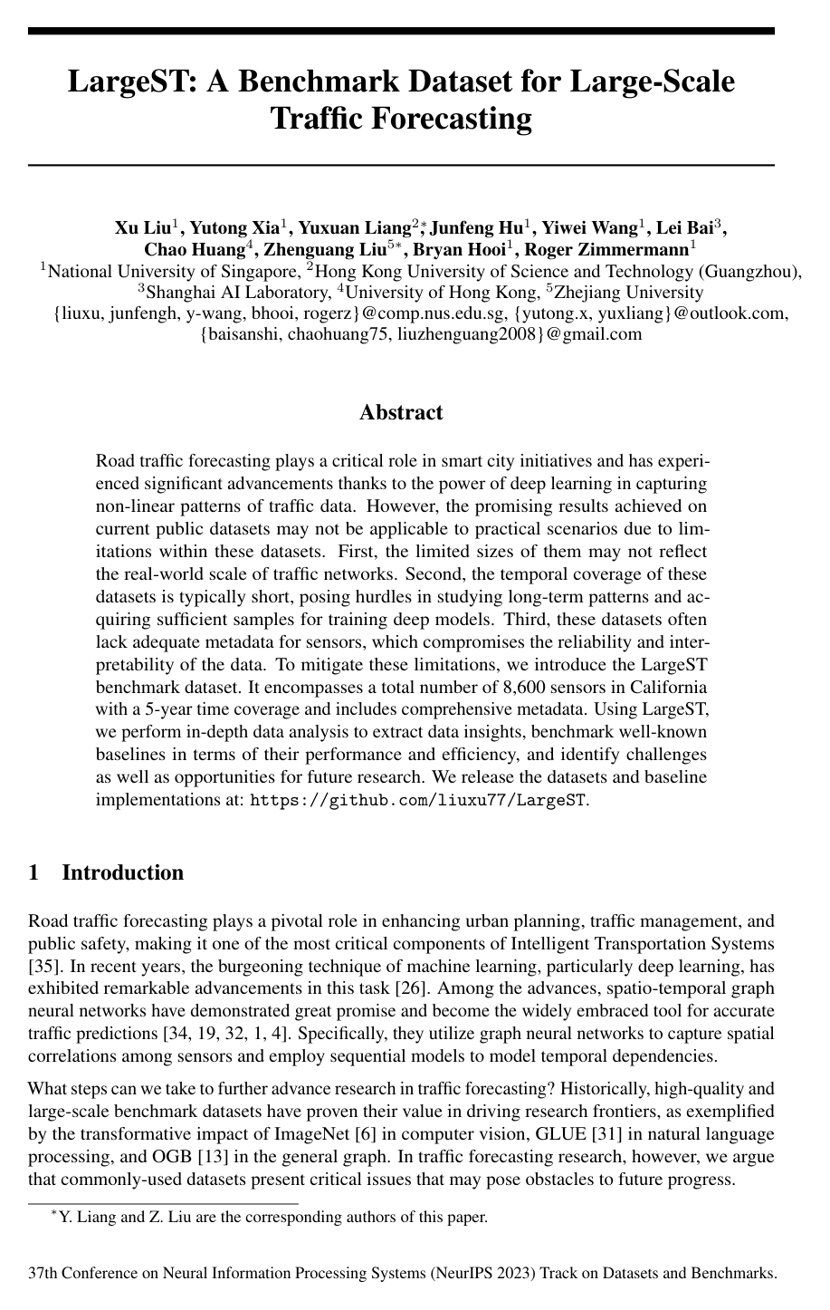
Cover for LargeST: A Benchmark Dataset for Large-Scale Traffic Forecasting

Abstract

Road traffic forecasting plays a critical role in smart city initiatives and has experienced significant advancements thanks to the power of deep learning in capturing non-linear patterns of traffic data. However, the promising results achieved on current public datasets may not be applicable to practical scenarios due to limitations within these datasets. First, the limited sizes of them may not reflect the real-world scale of traffic networks. Second, the temporal coverage of these datasets is typically short, posing hurdles in studying long-term patterns and acquiring sufficient samples for training deep models. Third, these datasets often lack adequate metadata for sensors, which compromises the reliability and interpretability of the data. To mitigate these limitations, we introduce the LargeST benchmark dataset. It encompasses a total number of 8,600 sensors in California with a 5-year time coverage and includes comprehensive metadata. Using LargeST, we perform in-depth data analysis to extract data insights, benchmark well-known baselines in terms of their performance and efficiency, and identify challenges as well as opportunities for future research. We release the datasets and baseline implementations at: https://github.com/liuxu77/LargeST.

Topics

deep learning dynamic traffic interpretability network traffic smart cities traffic networks vehicle density correlation analysis integrated data

Keywords

LargeST dataset large-scale traffic forecasting traffic flow forecasting benchmark dataset intelligent transportation systems road network

1 Introduction
2 Preliminaries
2.1 Problem Statement
2.2 Deep Learning-based Traffic Forecasting
3 Limitations of Existing Traffic Datasets
4 The LargeST Benchmark Dataset
4.1 Data Collection and Organization
4.2 Data Analysis
4.2.1 Regional Disparities
4.2.2 Temporal Dynamics
4.2.3 Metadata Characteristics
4.3 LargeST License
5 Experiments
5.1 Experimental Setup
5.2 Performance Comparisons
5.3 Efficiency Comparisons
6 Future Opportunities & Limitations
Acknowledgments and Disclosure of Funding
References
A Dataset Documentation
A.1 Motivation
A.2 Composition
A.3 Collection Process
A.4 Preprocessing/cleaning/labeling
A.5 Uses
A.6 Distribution
A.7 Maintenance
B More Dataset Information
C More Experimental Settings

Knowls

Knowl 1 — LargeST Benchmark Dataset Organization and Properties
definition
LargeST is a large-scale spatial-temporal traffic forecasting benchmark dataset based on traffic flow readings from loop detectors across the California state highway system, collected from the California Department of Transportation (CalTrans) Performance Measurement System (PeMS). The dataset encompasses $8{,}600$ mainline sensors observed continuously over a 5-year period from January 1, 2017 to December 31, 2021 at 5-minute sampling intervals ( $525{,}888$ time steps).

LargeST is organized into a hierarchical structure comprising the statewide dataset and three regional sub-datasets:
- California (CA): The full statewide network consisting of $8{,}600$ sensor nodes, $201{,}363$ directed edges, an average node degree of $23.4$ , a graph density of $0.0027$ , and $4.52$ billion total data points.
- Greater Los Angeles (GLA): Covers 5 counties (Los Angeles, Orange, Riverside, San Bernardino, Ventura) with $3{,}834$ sensor nodes, $98{,}703$ directed edges, an average node degree of $25.7$ , a graph density of $0.0067$ , and $2.02$ billion data points.
- Greater Bay Area (GBA): Covers 11 counties (Alameda, Contra Costa, Marin, Napa, San Benito, San Francisco, San Mateo, Santa Clara, Santa Cruz, Solano, Sonoma) with $2{,}352$ sensor nodes, $61{,}246$ directed edges, an average node degree of $26.0$ , a graph density of $0.0111$ , and $1.24$ billion data points.
- San Diego (SD): Covers San Diego county with $716$ sensor nodes, $17{,}319$ directed edges, an average node degree of $24.2$ , a graph density of $0.0338$ , and $0.38$ billion data points.
Knowl 2 — Graph Adjacency Matrix Construction with Geodesic Filtering and Routing Distances
model/method
To construct the directed graph adjacency matrix $A \in \mathbb{R}^{N \times N}$ for $N$ sensors, road network driving distances are determined using the Open Source Routing Machine (OSRM) on OpenStreetMap road network data. To avoid prohibitive $O(N^2)$ computational overhead for large sensor sets, pairwise geodesic distances are computed first, and exact road network driving distance queries are restricted to sensor pairs $(i, j)$ that fall within a 4-kilometer geodesic radius.

The edge weight between sensor $i$ and sensor $j$ is computed via a thresholded Gaussian kernel:

$A_{ij} = \begin{cases} \exp\left(-\frac{d_{ij}^2}{\sigma^2}\right), & \text{if } \exp\left(-\frac{d_{ij}^2}{\sigma^2}\right) \ge r \\ 0, & \text{otherwise} \end{cases}$

where $d_{ij}$ is the road network shortest driving distance between sensor $i$ and sensor $j$ , $\sigma$ denotes the standard deviation of all computed pairwise road network distances, and $r = 0.01$ is the edge pruning threshold used to remove weak connections.
Knowl 3 — Sensor Node Metadata Attributes
definition
Each sensor node in LargeST is accompanied by 9 metadata attributes:
1. ID: Unique sensor identifier in CalTrans PeMS (6 to 9-digit integer).
2. Lat: Latitude coordinate of the sensor.
3. Lng: Longitude coordinate of the sensor.
4. District: PeMS administrative district identifier (values: 3, 4, 5, 6, 7, 8, 10, 11, 12).
5. County: County in California where the sensor is located (covering 34 counties including Los Angeles, San Diego, Alameda, Santa Clara, etc.).
6. Fwy: Highway on which the sensor is installed (Interstates such as I5, I80, I405; U.S. Highways such as US101, US50; and State Routes such as SR99, SR52).
7. Lane: Number of highway lanes at the sensor point (ranging from 1 to 8).
8. Type: The sensor category, filtered exclusively to 'Mainline'.
9. Direction: Direction of highway traffic flow ('N', 'S', 'E', 'W').
Knowl 4 — Traffic Forecasting Benchmark Experimental Setup
experimental setup
The standard evaluation task on LargeST is spatial-temporal traffic forecasting: predicting target traffic flow values for the next 12 time steps based on the previous 12 historical time steps.

Raw 5-minute traffic readings are aggregated into 15-minute time intervals ( $96$ time steps per day). The evaluation benchmarks use one full year of data (2019) partitioned chronologically into training, validation, and test splits with a $6:2:2$ ratio, yielding sample sizes of $21{,}010$ (train), $7{,}003$ (validation), and $7{,}004$ (test) across all sub-datasets.

Evaluation is conducted using three metrics:
- Mean Absolute Error (MAE): $\text{MAE} = \frac{1}{M} \sum_{t=1}^M |y_t - \hat{y}_t|$
- Root Mean Squared Error (RMSE): $\text{RMSE} = \sqrt{\frac{1}{M} \sum_{t=1}^M (y_t - \hat{y}_t)^2}$
- Mean Absolute Percentage Error (MAPE): $\text{MAPE} = \frac{1}{M} \sum_{t=1}^M \left|\frac{y_t - \hat{y}_t}{y_t}\right| \times 100\%$
where $y_t$ and $\hat{y}_t$ denote ground truth and predicted values, and $M$ is the number of evaluated predictions. Performance is measured at prediction horizons 3 (45 min), 6 (90 min), and 12 (180 min), as well as averaged across all 12 horizons.

Knowl 5 — Benchmark Performance Comparisons across Models and Sub-Datasets

data/table

The table below details the performance of baseline models on the SD, GBA, GLA, and CA sub-datasets evaluated on 2019 traffic data. Missing entries on GLA and CA indicate out-of-memory (OOM) failures on a 48 GB NVIDIA RTX A6000 GPU even when the batch size was reduced to 4.

Data	Method	Param	Horizon 3			Horizon 6			Average
			MAE	RMSE	MAPE	MAE	RMSE	MAPE	MAE	RMSE	MAPE
SD	HL	–	33.61	50.97	20.77%	57.80	84.92	37.73%	60.79	87.40	41.88%
	LSTM	98K	19.03	30.53	11.81%	25.84	40.87	16.44%	26.44	41.73	17.20%
	DCRNN	373K	17.14	27.47	11.12%	20.99	33.29	13.95%	21.03	33.37	14.13%
	AGCRN	761K	15.71	27.85	11.48%	18.06	31.51	13.06%	18.09	32.01	13.28%
	STGCN	508K	17.45	29.99	12.42%	19.55	33.69	13.68%	19.67	34.14	13.86%
	GWNET	311K	15.24	25.13	9.86%	17.74	29.51	11.70%	17.74	29.62	11.88%
	ASTGCN	2.2M	19.56	31.33	12.18%	24.13	37.95	15.38%	23.70	37.63	15.65%
	STTN	114K	16.22	26.22	10.63%	18.76	30.98	12.80%	18.69	31.11	12.82%
	STGODE	729K	16.75	28.04	11.00%	19.71	33.56	13.16%	19.55	33.57	13.22%
	DSTAGNN	3.9M	18.13	28.96	11.38%	21.71	34.44	13.93%	21.82	34.68	14.40%
	DGCRN	243K	15.34	25.35	10.01%	18.05	30.06	11.90%	18.02	30.09	12.07%
	$\text{D}^2$ STGNN	406K	14.92	24.95	9.56%	17.52	29.24	11.36%	17.85	29.51	11.54%
GBA	DCRNN	373K	18.71	30.36	14.72%	23.06	36.16	20.45%	23.13	36.35	20.84%
	AGCRN	777K	18.31	30.24	14.27%	21.27	34.72	16.89%	21.01	34.25	16.90%
	STGCN	1.3M	21.05	34.51	16.42%	23.63	38.92	18.35%	23.42	38.57	18.46%
	GWNET	344K	17.85	29.12	13.92%	21.11	33.69	17.79%	20.91	33.41	17.66%
	DGCRN	374K	18.02	29.49	14.13%	21.08	34.03	16.94%	20.91	33.83	16.88%
	$\text{D}^2$ STGNN	446K	17.54	28.94	12.12%	20.92	33.92	14.89%	20.71	33.65	15.04%
GLA	DCRNN	373K	18.41	29.23	10.94%	23.16	36.15	14.14%	23.17	36.19	14.40%
	AGCRN	792K	17.27	29.70	10.78%	20.38	34.82	12.70%	20.25	34.84	12.87%
	STGCN	2.1M	19.86	34.10	12.40%	22.75	38.91	14.11%	22.64	38.81	14.17%
	GWNET	374K	17.28	27.68	10.18%	21.31	33.70	13.02%	21.20	33.58	13.18%
CA	DCRNN	373K	17.55	28.21	12.68%	21.79	34.27	16.67%	21.87	34.41	17.06%
	STGCN	4.5M	18.99	32.37	14.84%	21.37	36.46	16.27%	21.33	36.39	16.53%
	GWNET	469K	17.14	27.81	12.62%	21.68	34.16	17.14%	21.72	34.20	17.40%
	STGODE	1.0M	17.57	29.91	13.91%	20.98	36.62	16.88%	20.77	36.60	16.80%

Key takeaways:

Spatial-temporal GNNs consistently outperform non-spatial baselines (Historical Last and LSTM).
Models using adaptive adjacency matrices (GWNET, AGCRN) provide strong competitive accuracy while maintaining lower parameter scale and better computational efficiency.
Dynamic topology models (DGCRN, $\text{D}^2$ STGNN) achieve the strongest results on SD and GBA, but fail to scale to the larger GLA and CA subsets due to extreme GPU memory consumption.

Knowl 6 — Computational Efficiency and Hardware Scalability Benchmark

data/table

Computational efficiency evaluated on a single computing server equipped with an Intel Xeon Gold 6140 CPU @ 2.30 GHz, 376 GB RAM, and an NVIDIA RTX A6000 GPU (48 GB memory). Maximum initial batch size (BS) is capped at 64; if memory overflows, batch size is progressively halved down to 4.

Method	SD				GBA				GLA				CA
	BS	Train	Infer	Total	BS	Train	Infer	Total	BS	Train	Infer	Total	BS	Train	Infer	Total
LSTM	64	21	6	1	64	115	17	4	64	188	29	6	32	415	61	13
DCRNN	64	867	150	28	64	1,816	319	59	43	2,491	435	81	19	4,845	851	158
AGCRN	64	92	15	3	64	536	83	17	45	1,413	245	46	–	–	–	–
STGCN	64	53	16	2	64	160	54	6	64	268	86	10	64	701	206	25
GWNET	64	97	14	3	64	483	66	15	64	1,028	139	32	44	4,105	548	113
ASTGCN	64	128	19	4	45	1,126	147	35	17	3,060	393	77	–	–	–	–
STTN	64	208	26	6	7	1,758	197	50	–	–	–	–	–	–	–	–
STGODE	64	188	26	6	49	710	103	23	30	1,305	192	42	13	4,212	659	135
DSTAGNN	64	240	23	7	27	1,959	171	53	10	5,241	467	120	–	–	–	–
DGCRN	64	430	76	14	12	4,461	605	138	–	–	–	–	–	–	–	–
$\text{D}^2$ STGNN	45	563	69	14	4	5,885	796	148	–	–	–	–	–	–	–	–

Units: Train time is in seconds per epoch; Infer time is in seconds across the full validation set; Total is total training time in wall-clock hours.

Key efficiency findings:

TCN-based models (STGCN, GWNET) achieve superior execution speed and memory scaling due to parallel 1D temporal convolutions, running with batch size 64 across most datasets.
AGCRN is substantially faster than DCRNN due to its MLP-like decoder replacing the recurrent autoregressive decoder step.
Complex dynamic GNN architectures (DGCRN, $\text{D}^2$ STGNN, DSTAGNN, STTN) exhibit excessive memory footprints from intermediate graph representations, triggering OOM errors on GLA and CA subsets.

Knowl 7 — Spatio-Temporal Traffic Dynamics and Seasonal Distribution Shifts
empirical result
Empirical analysis of traffic flow patterns across LargeST indicates clear temporal and spatial distributions:
- Regional Disparities: Sensors in metropolitan sub-regions (GLA, GBA, and SD) display substantially higher average traffic flow volumes compared to the statewide CA average baseline.
- Daily Profiles: Weekday traffic displays a pronounced bimodal distribution with a morning peak around 8:00 AM and an evening peak around 5:00 PM. Weekend traffic follows a distinct unimodal profile with steady volume across the afternoon.
- Peak Variance: The morning peak exhibits greater flow variance than the evening peak, reflecting flexibility in morning departure times relative to uniform evening congestion.
- Annual Seasonality: Peak traffic volumes exhibit an annual distribution shift across months: flow increases steadily from January to May, fluctuates at elevated levels between June and September, and declines gradually from October through December.
Knowl 8 — Correlation of Highway Types and Lane Counts with Traffic Flow
empirical result
Analysis of the metadata distributions across the $8{,}600$ sensors in the CA dataset demonstrates:
- Highway Classification: Interstate highways represent the majority ( $4{,}322$ sensors), followed by State Routes ( $3{,}044$ sensors) and U.S. Highways ( $1{,}234$ sensors). Interstate highways display the highest average traffic flow volume due to intercity and freight transit demands, followed by U.S. Highways, while State Routes have the lowest average volume.
- Highway Lane Distribution: Sensors are predominantly installed on 3-to-4 lane road segments ( $5{,}679$ in CA, $2{,}769$ in GLA, $1{,}459$ in GBA, $449$ in SD), with 1-to-2 lanes ( $1{,}347$ in CA) and $\ge 5$ lanes ( $1{,}574$ in CA) making up the remainder.
- Capacity Correlation: A positive monotonic correlation exists between the number of lanes and average recorded traffic volume, attributable to higher physical vehicular capacity.
Knowl 9 — Limitations of LargeST
limitation
The LargeST benchmark presents two primary limitations:
1. Geographic Generalizability: All sensor nodes, traffic flows, and topology graphs originate strictly from the California state highway system, which may not directly generalize to road network structures, driving patterns, or traffic rules in other geographic regions.
2. Sensor Missingness and Data Artifacts: Real-world loop detectors suffer from signal interruptions and hardware dropouts. To preserve raw operational conditions, LargeST does not filter out sensors with missing readings or apply artificial data imputation, requiring downstream users to implement interpolation if desired.

Coverage note — None was omitted; all contributed datasets, graph building methods, metadata properties, experimental benchmarks, empirical findings, and stated limitations are fully covered.

References

1.Lei Bai, Lina Yao, Can Li, Xianzhi Wang, and Can Wang. Adaptive graph convolutional recurrent network for traffic forecasting. In Proceedings of Advances in Neural Information Processing Systems, pages 17804–17815, 2020.
2.Defu Cao, Yujing Wang, Juanyong Duan, Ce Zhang, Xia Zhu, Congrui Huang, Yunhai Tong, Bixiong Xu, Jing Bai, Jie Tong, et al. Spectral temporal graph neural network for multivariate time-series forecasting. In Proceedings of Advances in Neural Information Processing Systems, pages 17766–17778, 2020.
3.Chao Chen, Karl Petty, Alexander Skabardonis, Pravin Varaiya, and Zhanfeng Jia. Freeway performance measurement system: mining loop detector data. Transportation research record, pages 96–102, 2001.
4.Jeongwhan Choi, Hwangyong Choi, Jeehyun Hwang, and Noseong Park. Graph neural controlled differential equations for traffic forecasting. In Proceedings of the AAAI Conference on Artificial Intelligence, pages 6367–6374, 2022.
5.Michaël Defferrard, Xavier Bresson, and Pierre Vandergheynst. Convolutional neural networks on graphs with fast localized spectral filtering. In Proceedings of Advances in Neural Information Processing Systems, pages 3837–3845, 2016.
6.Jia Deng, Wei Dong, Richard Socher, Li-Jia Li, Kai Li, and Li Fei-Fei. Imagenet: A large-scale hierarchical image database. In IEEE conference on computer vision and pattern recognition, pages 248–255, 2009.
7.Yuchen Fang, Yanjun Qin, Haiyong Luo, Fang Zhao, Bingbing Xu, Liang Zeng, and Chenxing Wang. When spatio-temporal meet wavelets: Disentangled traffic forecasting via efficient spectral graph attention networks. In 2023 IEEE 39th International Conference on Data Engineering (ICDE), pages 517–529, 2023.
8.Zheng Fang, Qingqing Long, Guojie Song, and Kunqing Xie. Spatial-temporal graph ode networks for traffic flow forecasting. In Proceedings of the 27th ACM SIGKDD Conference on Knowledge Discovery and Data Mining, pages 364–373, 2021.
9.Timnit Gebru, Jamie Morgenstern, Briana Vecchione, Jennifer Wortman Vaughan, Hanna Wallach, Hal Daumé Iii, and Kate Crawford. Datasheets for datasets. Communications of the ACM, pages 86–92, 2021.
10.Shengnan Guo, Youfang Lin, Ning Feng, Chao Song, and Huaiyu Wan. Attention based spatial-temporal graph convolutional networks for traffic flow forecasting. In Proceedings of the AAAI Conference on Artificial Intelligence, pages 922–929, 2019.
11.Liangzhe Han, Bowen Du, Leilei Sun, Yanjie Fu, Yisheng Lv, and Hui Xiong. Dynamic and multi-faceted spatio-temporal deep learning for traffic speed forecasting. In Proceedings of the 27th ACM SIGKDD Conference on Knowledge Discovery and Data Mining, pages 547–555, 2021.
12.Sepp Hochreiter and Jürgen Schmidhuber. Long short-term memory. Neural computation, pages 1735–1780, 1997.
13.Weihua Hu, Matthias Fey, Marinka Zitnik, Yuxiao Dong, Hongyu Ren, Bowen Liu, Michele Catasta, and Jure Leskovec. Open graph benchmark: Datasets for machine learning on graphs. In Proceedings of Advances in Neural Information Processing Systems, pages 22118–22133, 2020.
14.Thomas N Kipf and Max Welling. Semi-supervised classification with graph convolutional networks. In International Conference on Learning Representations, 2017.
15.Jake Kononov, Barbara Bailey, and Bryan K Allery. Relationships between safety and both congestion and number of lanes on urban freeways. Transportation research record, pages 26–39, 2008.
16.Jake Kononov, David Reeves, Catherine Durso, and Bryan K Allery. Relationship between freeway flow parameters and safety and its implication for adding lanes. Transportation research record, pages 118–123, 2012.
17.Shiyong Lan, Yitong Ma, Weikang Huang, Wenwu Wang, Hongyu Yang, and Pyang Li. Dstagnn: Dynamic spatial-temporal aware graph neural network for traffic flow forecasting. In International Conference on Machine Learning, pages 11906–11917, 2022.
18.Fuxian Li, Jie Feng, Huan Yan, Guangyin Jin, Fan Yang, Funing Sun, Depeng Jin, and Yong Li. Dynamic graph convolutional recurrent network for traffic prediction: Benchmark and solution. ACM Transactions on Knowledge Discovery from Data, pages 1–21, 2021.
19.Yaguang Li, Rose Yu, Cyrus Shahabi, and Yan Liu. Diffusion convolutional recurrent neural network: Data-driven traffic forecasting. In International Conference on Learning Representations, 2018.
20.Yuxuan Liang, Songyu Ke, Junbo Zhang, Xiuwen Yi, and Yu Zheng. Geoman: Multi-level attention networks for geo-sensory time series prediction. In Proceedings of International Joint Conference on Artificial Intelligence, pages 3428–3434, 2018.
21.Yuxuan Liang, Kun Ouyang, Yiwei Wang, Ye Liu, Junbo Zhang, Yu Zheng, and David S Rosenblum. Revisiting convolutional neural networks for citywide crowd flow analytics. In Proceedings of European Conference on Machine Learning and Principles and Practice of Knowledge Discovery, pages 578–594, 2021.
22.Xu Liu, Yuxuan Liang, Chao Huang, Yu Zheng, Bryan Hooi, and Roger Zimmermann. When do contrastive learning signals help spatio-temporal graph forecasting? In Proceedings of the 30th International Conference on Advances in Geographic Information Systems, pages 1–12, 2022.
23.Xu Liu, Yuxuan Liang, Chao Huang, Hengchang Hu, Yushi Cao, Bryan Hooi, and Roger Zimmermann. Do we really need graph neural networks for traffic forecasting? arXiv preprint arXiv:2301.12603, 2023.
24.Dennis Luxen and Christian Vetter. Real-time routing with openstreetmap data. In Proceedings of the 19th ACM SIGSPATIAL international conference on advances in geographic information systems, pages 513–516, 2011.
25.Tanwi Mallick, Prasanna Balaprakash, Eric Rask, and Jane Macfarlane. Graph-partitioning-based diffusion convolutional recurrent neural network for large-scale traffic forecasting. Transportation Research Record, pages 473–488, 2020.
26.Eric L Manibardo, Ibai Laña, and Javier Del Ser. Deep learning for road traffic forecasting: Does it make a difference? IEEE Transactions on Intelligent Transportation Systems, pages 6164–6188, 2021.
27.Zheyi Pan, Yuxuan Liang, Weifeng Wang, Yong Yu, Yu Zheng, and Junbo Zhang. Urban traffic prediction from spatio-temporal data using deep meta learning. In Proceedings of the 25th ACM SIGKDD Conference on Knowledge Discovery and Data Mining, pages 1720–1730, 2019.
28.Zezhi Shao, Zhao Zhang, Wei Wei, Fei Wang, Yongjun Xu, Xin Cao, and Christian S Jensen. Decoupled dynamic spatial-temporal graph neural network for traffic forecasting. In Proceedings of the VLDB Endowment, pages 2733–2746, 2022.
29.David I Shuman, Sunil K Narang, Pascal Frossard, Antonio Ortega, and Pierre Vandergheynst. The emerging field of signal processing on graphs: Extending high-dimensional data analysis to networks and other irregular domains. IEEE Signal Processing Magazine, pages 83–98, 2013.
30.Chao Song, Youfang Lin, Shengnan Guo, and Huaiyu Wan. Spatial-temporal synchronous graph convolutional networks: A new framework for spatial-temporal network data forecasting. In Proceedings of the AAAI Conference on Artificial Intelligence, pages 914–921, 2020.
31.Alex Wang, Amanpreet Singh, Julian Michael, Felix Hill, Omer Levy, and Samuel R Bowman. Glue: A multi-task benchmark and analysis platform for natural language understanding. In International Conference on Learning Representations, 2019.
32.Zonghan Wu, Shirui Pan, Guodong Long, Jing Jiang, and Chengqi Zhang. Graph wavenet for deep spatial-temporal graph modeling. In Proceedings of International Joint Conference on Artificial Intelligence, pages 1907–1913, 2019.
33.Mingxing Xu, Wenrui Dai, Chunmiao Liu, Xing Gao, Weiyao Lin, Guo-Jun Qi, and Hongkai Xiong. Spatial-temporal transformer networks for traffic flow forecasting. arXiv preprint arXiv:2001.02908, 2020.
34.Bing Yu, Haoteng Yin, and Zhanxing Zhu. Spatio-temporal graph convolutional networks: A deep learning framework for traffic forecasting. In Proceedings of International Joint Conference on Artificial Intelligence, pages 3634–3640, 2018.
35.Yu Zheng, Licia Capra, Ouri Wolfson, and Hai Yang. Urban computing: concepts, methodologies, and applications. ACM Transactions on Intelligent Systems and Technology (TIST), pages 1–55, 2014.

Citation

MLA

Liu, X., et al. “LargeST: A Benchmark Dataset for Large-Scale Traffic Forecasting”. arXiv, 2023, http://arxiv.org/abs/2306.08259v2.

APA

Liu, X., Xia, Y., Liang, Y., Hu, J., Wang, Y., Bai, L., Huang, C., Liu, Z., Hooi, B., & Zimmermann, R. (2023). LargeST: A Benchmark Dataset for Large-Scale Traffic Forecasting. arXiv. http://arxiv.org/abs/2306.08259v2

Chicago

Liu, X., Y. Xia, Y. Liang, et al. 2023. “LargeST: A Benchmark Dataset for Large-Scale Traffic Forecasting”. arXiv. http://arxiv.org/abs/2306.08259v2.

Harvard

Liu, X. et al. (2023) “LargeST: A Benchmark Dataset for Large-Scale Traffic Forecasting”, arXiv [Preprint]. Available at: http://arxiv.org/abs/2306.08259v2.

Vancouver

1. Liu X, Xia Y, Liang Y, Hu J, Wang Y, Bai L, Huang C, Liu Z, Hooi B, Zimmermann R (2023) LargeST: A Benchmark Dataset for Large-Scale Traffic Forecasting. arXiv

BibTeX

@article{liu2023largest,
  title = {LargeST: A Benchmark Dataset for Large-Scale Traffic Forecasting},
  author = {Liu, Xu and Xia, Yutong and Liang, Yuxuan and Hu, Junfeng and Wang, Yiwei and Bai, Lei and Huang, Chao and Liu, Zhenguang and Hooi, Bryan and Zimmermann, Roger},
  year = {2023},
  journal = {arXiv},
  url = {http://arxiv.org/abs/2306.08259v2},
  eprint = {2306.08259}
}

Metadata:arXiv

Source Code

This paper has an official code repository available. Click below to access the source code.

View Repository

Access the Paper

This paper is available from its original source. Click below to access the PDF.

Open PDF

License: Authors

LargeST: A Benchmark Dataset for Large-Scale Traffic Forecasting

Abstract

Topics

Keywords

Table of Contents

Knowls

Knowl 1 — LargeST Benchmark Dataset Organization and Properties

Knowl 2 — Graph Adjacency Matrix Construction with Geodesic Filtering and Routing Distances

Knowl 3 — Sensor Node Metadata Attributes

Knowl 4 — Traffic Forecasting Benchmark Experimental Setup