Attention Based Spatial-Temporal Graph Convolutional Networks for Traffic Flow Forecasting

Shengnan GuoYoufang LinNing FengChao SongHuaiyu Wan

article2019AAAI3,347 citations

Proposes an attention-based spatial-temporal graph convolutional network that integrates dynamic spatial-temporal attention mechanisms with graph convolutions to model multi-periodic dependencies and achieve superior traffic flow forecasting on highway networks.

Listen

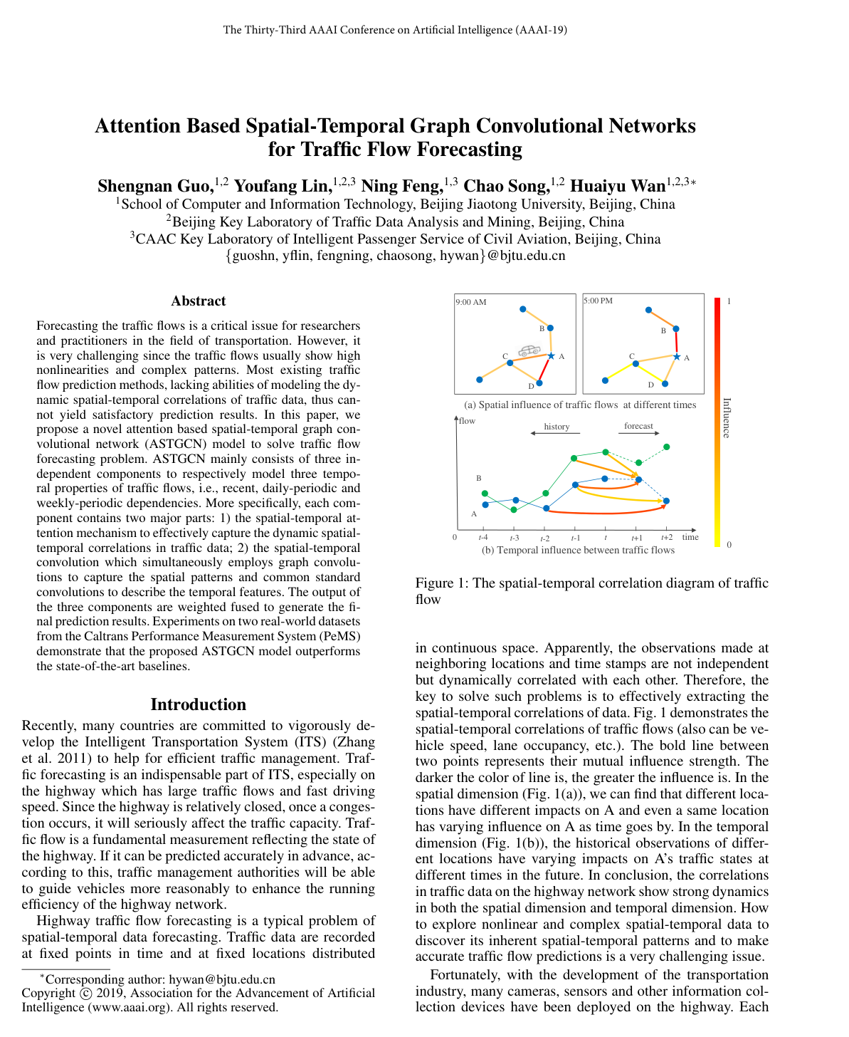
Traffic flow forecasting supports efficient highway management within intelligent transportation systems, yet remains difficult because traffic data exhibit strong nonlinear patterns and dynamic correlations that shift across both locations and time periods. Traditional time-series models and early deep-learning approaches often fail to capture these spatial-temporal dependencies simultaneously, leading to limited accuracy especially over longer prediction horizons.

This paper introduces the Attention-based Spatial-Temporal Graph Convolutional Network (ASTGCN) to address that gap. The model processes traffic data directly on the original sensor graph and explicitly models three temporal scalesrecent, daily-periodic, and weekly-periodicbefore fusing their outputs.

The approach combines a spatial-temporal attention mechanism with graph convolutions in space and standard convolutions in time. Three parallel components, each built from stacked spatial-temporal blocks, learn dynamic node-to-node and time-to-time influences; the components are then merged through learned per-node weights. Experiments used two real-world highway datasets from the California PeMS system (PeMSD4 with 307 detectors over two months in 2018 and PeMSD8 with 170 detectors over two months in 2016), with traffic aggregated every five minutes and missing values imputed by linear interpolation.

On both datasets ASTGCN produced the lowest root-mean-square and mean-absolute errors for one-hour-ahead forecasts, outperforming eight baselines that included ARIMA, LSTM, GRU, STGCN, GLU-STGCN, and GeoMAN. The version without attention (MSTGCN) already surpassed prior state-of-the-art models, and adding attention yielded a further consistent reduction in error. Gains were largest at longer prediction intervals, and the learned attention matrices aligned with actual geographic proximity, providing a degree of interpretability.

These results indicate that explicitly modeling dynamic spatial-temporal correlations can materially improve forecast reliability, supporting more timely congestion management and better use of highway capacity. Because the framework operates on arbitrary graph-structured sensor networks, it can be extended to related tasks such as arrival-time estimation.

The authors note that external influences such as weather or events are not yet incorporated and recommend including them in future work. The current evaluation is limited to two California corridors; broader geographic validation and sensitivity checks on sensor density would increase confidence for operational deployment.

Cover for Attention Based Spatial-Temporal Graph Convolutional Networks for Traffic Flow Forecasting

Abstract

Forecasting the traffic flows is a critical issue for researchers and practitioners in the field of transportation. However, it is very challenging since the traffic flows usually show high nonlinearities and complex patterns. Most existing traffic flow prediction methods, lacking abilities of modeling the dynamic spatial-temporal correlations of traffic data, thus cannot yield satisfactory prediction results. In this paper, we propose a novel attention based spatial-temporal graph convolutional network (ASTGCN) model to solve traffic flow forecasting problem. ASTGCN mainly consists of three independent components to respectively model three temporal properties of traffic flows, i.e., recent, daily-periodic and weekly-periodic dependencies. More specifically, each component contains two major parts: 1) the spatial-temporal attention mechanism to effectively capture the dynamic spatial-temporal correlations in traffic data; 2) the spatial-temporal convolution which simultaneously employs graph convolutions to capture the spatial patterns and common standard convolutions to describe the temporal features. The output of the three components are weighted fused to generate the final prediction results. Experiments on two real-world datasets from the Caltrans Performance Measurement System (PeMS) demonstrate that the proposed ASTGCN model outperforms the state-of-the-art baselines.

Table of Contents

  • Introduction
  • Related work
  • Preliminaries
  • Traffic Networks
  • Traffic Flow Forecasting
  • Attention Based Spatial-Temporal Graph Convolutional Networks
  • Spatial-Temporal Attention
  • Spatial-Temporal Convolution
  • Multi-Component Fusion
  • Experiments
  • Datasets
  • Preprocessing
  • Settings
  • Baselines
  • Comparison and Result Analysis
  • Conclusion and Future Work
  • Acknowledgments
  • References

Knowls

  1. Knowl 1 — Attention Based Spatial-Temporal Graph Convolutional Network Architecture

    model/method

    The Attention Based Spatial-Temporal Graph Convolutional Network (ASTGCN) is designed to collectively forecast future traffic flows across all nodes on a road network graph G=(V,E,A)G = (V, E, A) over a forecasting horizon TpT_p. ASTGCN contains three parallel components sharing identical internal architectures, each modeling a distinct temporal property:

    1. Recent component: Receives input XhRN×F×Th\mathcal{X}_h \in \mathbb{R}^{N \times F \times T_h} to model short-term traffic trend dependencies.
    2. Daily-periodic component: Receives input XdRN×F×Td\mathcal{X}_d \in \mathbb{R}^{N \times F \times T_d} to capture repeating daily patterns (e.g., morning and evening peak hours).
    3. Weekly-periodic component: Receives input XwRN×F×Tw\mathcal{X}_w \in \mathbb{R}^{N \times F \times T_w} to capture weekday-versus-weekend recurrence.

    Each component consists of a sequence of stacked Spatial-Temporal (ST) blocks with residual connections, followed by a fully-connected layer. Within each ST block:

    • A Spatial-Temporal Attention module dynamically computes spatial attention weights across nodes and temporal attention weights across time slices from current features.
    • A Spatial-Temporal Convolution module applies spectral Chebyshev graph convolutions modulated by the spatial attention matrix to capture network topology, followed by 1D temporal convolutions along the time dimension.

    The output traffic predictions Y^h,Y^d,Y^wRN×Tp\hat{Y}_h, \hat{Y}_d, \hat{Y}_w \in \mathbb{R}^{N \times T_p} from the three components are merged via a learnable parameter-weighted Hadamard fusion layer to produce the final network prediction Y^RN×Tp\hat{Y} \in \mathbb{R}^{N \times T_p}.

  2. Knowl 2 — Spatial and Temporal Attention Mechanisms in ASTGCN

    model/method

    To dynamically capture time-varying correlations between sensor nodes and across time slices, each Spatial-Temporal block in ASTGCN incorporates spatial and temporal attention mechanisms.

    Spatial Attention: Given the input feature tensor X(r1)RN×Cr1×Tr1X^{(r-1)} \in \mathbb{R}^{N \times C_{r-1} \times T_{r-1}} to the rr-th ST block (where NN is the number of nodes, Cr1C_{r-1} is the channel dimension, and Tr1T_{r-1} is the temporal length), the dynamic spatial correlation matrix SRN×NS \in \mathbb{R}^{N \times N} and its normalized counterpart SRN×NS' \in \mathbb{R}^{N \times N} are computed as:

    S=Vsσ((X(r1)W1)W2(W3X(r1))T+bs)S = V_s \cdot \sigma \left( (X^{(r-1)} W_1) W_2 (W_3 X^{(r-1)})^T + b_s \right)

    Si,j=exp(Si,j)j=1Nexp(Si,j)S'_{i,j} = \frac{\exp(S_{i,j})}{\sum_{j=1}^N \exp(S_{i,j})}

    where W1RTr1W_1 \in \mathbb{R}^{T_{r-1}}, W2RCr1×Tr1W_2 \in \mathbb{R}^{C_{r-1} \times T_{r-1}}, W3RCr1W_3 \in \mathbb{R}^{C_{r-1}}, and Vs,bsRN×NV_s, b_s \in \mathbb{R}^{N \times N} are learnable parameters, and σ()\sigma(\cdot) is the sigmoid activation function.

    Temporal Attention: To adaptively weight the importance of different time slices, the temporal correlation matrix ERTr1×Tr1E \in \mathbb{R}^{T_{r-1} \times T_{r-1}} and its normalized counterpart ERTr1×Tr1E' \in \mathbb{R}^{T_{r-1} \times T_{r-1}} are calculated as:

    E=Veσ(((X(r1))TU1)U2(U3X(r1))+be)E = V_e \cdot \sigma \left( ((X^{(r-1)})^T U_1) U_2 (U_3 X^{(r-1)}) + b_e \right)

    Ei,j=exp(Ei,j)j=1Tr1exp(Ei,j)E'_{i,j} = \frac{\exp(E_{i,j})}{\sum_{j=1}^{T_{r-1}} \exp(E_{i,j})}

    where U1RNU_1 \in \mathbb{R}^N, U2RCr1×NU_2 \in \mathbb{R}^{C_{r-1} \times N}, U3RCr1U_3 \in \mathbb{R}^{C_{r-1}}, and Ve,beRTr1×Tr1V_e, b_e \in \mathbb{R}^{T_{r-1} \times T_{r-1}} are learnable parameters. The temporal attention is applied directly to adjust the input tensor via matrix multiplication:

    X^(r1)=X(r1)ERN×Cr1×Tr1\hat{X}^{(r-1)} = X^{(r-1)} E' \in \mathbb{R}^{N \times C_{r-1} \times T_{r-1}}

  3. Knowl 3 — Chebyshev Graph Convolution with Spatial Attention

    model/method

    ASTGCN models topological spatial interactions across the road graph G=(V,E,A)G = (V, E, A) using spectral graph convolutions approximated by truncated Chebyshev polynomials and dynamically adjusted by the spatial attention matrix SS'.

    Let L=IND1/2AD1/2RN×NL = I_N - D^{-1/2} A D^{-1/2} \in \mathbb{R}^{N \times N} be the normalized Graph Laplacian, where AA is the adjacency matrix, INI_N is the identity matrix, and DD is the diagonal degree matrix (Dii=jAijD_{ii} = \sum_j A_{ij}). The scaled Laplacian is defined as L~=2λmaxLIN\tilde{L} = \frac{2}{\lambda_{\max}} L - I_N, where λmax\lambda_{\max} is the maximum eigenvalue of LL.

    To capture localized spatial features up to (K1)(K-1)-th order neighbors while incorporating dynamic node correlations, each Chebyshev polynomial term Tk(L~)T_k(\tilde{L}) is modulated by the spatial attention matrix SRN×NS' \in \mathbb{R}^{N \times N} via the Hadamard product:

    gθGx=k=0K1θk(Tk(L~)S)xg_\theta *_G x = \sum_{k=0}^{K-1} \theta_k \left( T_k(\tilde{L}) \odot S' \right) x

    where \odot is the Hadamard (element-wise) product, θRK\theta \in \mathbb{R}^K is a vector of polynomial coefficients, and the Chebyshev polynomials are recursively computed as: T0(x)=1,T1(x)=x,Tk(x)=2xTk1(x)Tk2(x)(k2)T_0(x) = 1, \quad T_1(x) = x, \quad T_k(x) = 2x T_{k-1}(x) - T_{k-2}(x) \quad (k \ge 2)

    For a multi-channel signal X^tRN×Cr1\hat{X}_t \in \mathbb{R}^{N \times C_{r-1}} at time step tt, performing CrC_r filters parameterized by kernel weights ΘRK×Cr1×Cr\Theta \in \mathbb{R}^{K \times C_{r-1} \times C_r} yields the updated feature representation for each node.

  4. Knowl 4 — Temporal Convolution in Spatial-Temporal Blocks

    equation

    Following the attention-augmented graph convolution in the spatial dimension, ASTGCN applies a standard 1D convolution across the temporal dimension to aggregate information from adjacent time steps.

    For the rr-th spatial-temporal block with temporally-attended input X^(r1)RN×Cr1×Tr1\hat{X}^{(r-1)} \in \mathbb{R}^{N \times C_{r-1} \times T_{r-1}}, the complete spatial-temporal convolution operation is defined as:

    X(r)=ReLU(Φ(ReLU(gθGX^(r1))))RCr×N×TrX^{(r)} = \text{ReLU}\left( \Phi * \left( \text{ReLU}\left( g_\theta *_G \hat{X}^{(r-1)} \right) \right) \right) \in \mathbb{R}^{C_r \times N \times T_r}

    where:

    • G*_G denotes the Chebyshev spectral graph convolution modulated by the spatial attention matrix SS'.
    • * denotes standard 1D convolution along the temporal dimension.
    • Φ\Phi represents the learnable parameters of the temporal convolution kernel.
    • ReLU(z)=max(0,z)\text{ReLU}(z) = \max(0, z) is the activation function.
    • CrC_r is the number of feature channels in the rr-th layer, NN is the number of nodes, and TrT_r is the resulting temporal sequence length.
  5. Knowl 5 — Multi-Period Input Segment Construction

    definition

    For a traffic sensor network with daily sampling frequency qq (time slices per day), current time t0t_0, and forecasting horizon TpT_p, ASTGCN constructs three distinct input time series segments along the time axis:

    1. Recent Segment (XhRN×F×Th\mathcal{X}_h \in \mathbb{R}^{N \times F \times T_h}): Comprises ThT_h consecutive time slices directly preceding t0t_0: Xh=(Xt0Th+1,Xt0Th+2,,Xt0)\mathcal{X}_h = (X_{t_0 - T_h + 1}, X_{t_0 - T_h + 2}, \ldots, X_{t_0})

    2. Daily-Periodic Segment (XdRN×F×Td\mathcal{X}_d \in \mathbb{R}^{N \times F \times T_d}): Comprises segments from the preceding Td/TpT_d / T_p days covering the same time of day as the prediction window: Xd=(Xt0(Td/Tp)q+1,,Xt0(Td/Tp)q+Tp,,Xt0q+1,,Xt0q+Tp)\mathcal{X}_d = (X_{t_0 - (T_d / T_p) q + 1}, \ldots, X_{t_0 - (T_d / T_p) q + T_p}, \ldots, X_{t_0 - q + 1}, \ldots, X_{t_0 - q + T_p})

    3. Weekly-Periodic Segment (XwRN×F×Tw\mathcal{X}_w \in \mathbb{R}^{N \times F \times T_w}): Comprises segments from the preceding Tw/TpT_w / T_p weeks at the same time interval on the same day of the week: Xw=(Xt07(Tw/Tp)q+1,,Xt07(Tw/Tp)q+Tp,,Xt07q+1,,Xt07q+Tp)\mathcal{X}_w = (X_{t_0 - 7 (T_w / T_p) q + 1}, \ldots, X_{t_0 - 7 (T_w / T_p) q + T_p}, \ldots, X_{t_0 - 7 q + 1}, \ldots, X_{t_0 - 7 q + T_p})

    Here, NN is the number of sensor nodes, FF is the number of measurement features per node, and Th,Td,TwT_h, T_d, T_w are positive integers that are integer multiples of TpT_p.

  6. Knowl 6 — Multi-Component Output Fusion

    equation

    The output representations from the recent, daily-periodic, and weekly-periodic components (Y^h,Y^d,Y^wRN×Tp\hat{Y}_h, \hat{Y}_d, \hat{Y}_w \in \mathbb{R}^{N \times T_p}) are combined using a learnable parameter matrix to obtain the final forecasted traffic flows Y^RN×Tp\hat{Y} \in \mathbb{R}^{N \times T_p}:

    Y^=WhY^h+WdY^d+WwY^w\hat{Y} = W_h \odot \hat{Y}_h + W_d \odot \hat{Y}_d + W_w \odot \hat{Y}_w

    where:

    • \odot represents the Hadamard (element-wise) product.
    • Wh,Wd,WwRN×TpW_h, W_d, W_w \in \mathbb{R}^{N \times T_p} are learnable weight matrices that adaptively calibrate the relative contribution of each temporal component for every individual sensor node and prediction horizon time step.
    • NN is the number of traffic sensors and TpT_p is the forecasting window length.
  7. Knowl 7 — Traffic Flow Forecasting Performance Comparison

    data/table

    The traffic flow prediction performance of ASTGCN was evaluated against eight baseline models on two highway datasets (PeMSD4 and PeMSD8) over a 1-hour future horizon (Tp=12T_p = 12 time slices of 5 minutes). Metrics are Root Mean Square Error (RMSE) and Mean Absolute Error (MAE).

    Model PeMSD4 PeMSD8
    RMSE MAE RMSE MAE
    HA 54.14 36.76 44.03 29.52
    ARIMA 68.13 32.11 43.30 24.04
    VAR 51.73 33.76 31.21 21.41
    LSTM 45.82 29.45 36.96 23.18
    GRU 45.11 28.65 35.95 22.20
    STGCN 38.29 25.15 27.87 18.88
    GLU-STGCN 38.41 27.28 30.78 20.99
    GeoMAN 37.84 23.64 28.91 17.84
    MSTGCN (ours) 35.64 22.73 26.47 17.47
    ASTGCN (ours) 32.82 21.80 25.27 16.63

    ASTGCN achieves the lowest error across all metrics on both datasets. Comparing models shows that:

    1. Deep learning models jointly considering spatial and temporal dependencies (STGCN, GLU-STGCN, GeoMAN, MSTGCN, ASTGCN) outperform purely temporal statistical and recurrent models (HA, ARIMA, VAR, LSTM, GRU).
    2. MSTGCN (the degraded version without spatial-temporal attention) outperforms all prior baselines, showing the benefit of the multi-component spatial-temporal architecture.
    3. ASTGCN achieves further error reduction over MSTGCN (reducing RMSE from 35.64 to 32.82 on PeMSD4 and from 26.47 to 25.27 on PeMSD8), verifying the efficacy of the spatial-temporal attention mechanism.
  8. Knowl 8 — Experimental Setup and Datasets for ASTGCN Evaluation

    experimental setup

    ASTGCN is evaluated on two Caltrans Performance Measurement System (PeMS) highway traffic datasets aggregated into 5-minute intervals (q=288q = 288 points per detector per day):

    • PeMSD4: San Francisco Bay Area (January–February 2018), containing 307 detectors across 29 roads after removing redundant detectors spaced closer than 3.5 miles. The first 50 days form the training set and the remainder the test set.
    • PeMSD8: San Bernardino (July–August 2016), containing 170 detectors across 8 roads (filtered to >3.5>3.5 mile spacing). The first 50 days serve as the training set and the final 12 days as the test set.

    Each detector records F=3F = 3 traffic measurements: total flow, average speed, and average occupancy. Missing values are imputed via linear interpolation, and features are standardized via zero-mean normalization x=xmean(x)x' = x - \text{mean}(x).

    Hyperparameters and Training Details:

    • Prediction window: Tp=12T_p = 12 time slices (1 hour).
    • Input segment lengths: Th=24T_h = 24, Td=12T_d = 12, Tw=24T_w = 24.
    • Chebyshev polynomial order: K=3K = 3.
    • Convolution filters: 64 kernels for all graph convolution layers; 64 kernels for all temporal convolution layers with temporal kernel size of 3.
    • Training parameters: Mean Squared Error (MSE) loss, batch size of 64, learning rate of 0.0001, optimized using backpropagation in MXNet.
  9. Knowl 9 — Impact of Prediction Horizon on Traffic Forecasting Accuracy

    empirical result

    Evaluating prediction performance across increasing forecasting horizons from 5 to 60 minutes (1 to 12 prediction steps) reveals distinct model behaviors:

    • Purely temporal models (HA, ARIMA, LSTM, GRU) perform adequately on immediate next-step prediction (5 minutes) but suffer steep degradation in accuracy as the prediction horizon lengthens.
    • Vector Auto-Regressive (VAR) models degrade more slowly with horizon length because they capture spatial cross-correlations; however, VAR error escalates dramatically when scaling to larger network sizes (PeMSD4 with 307 detectors vs. PeMSD8 with 170 detectors).
    • Deep spatial-temporal architectures maintain slower error growth rates across time horizons.
    • ASTGCN consistently achieves the lowest RMSE and MAE at all prediction steps, and its performance advantage over baseline models becomes increasingly pronounced at longer prediction horizons (e.g., at 45–60 minutes).
  10. Knowl 10 — Interpretability of Learned Spatial Attention Weights

    empirical result

    A case study on a sub-graph of 10 detectors from PeMSD8 demonstrates the physical interpretability of ASTGCN's spatial attention mechanism:

    • The learned spatial attention matrix SS' assigns substantially higher attention weights between pairs of detectors that are geographically close and connected along the same highway corridor (e.g., detector 9 exhibits strong attention weights toward adjacent detectors 3 and 8).
    • This demonstrates that the spatial attention module automatically discovers and reflects true spatial network topology from traffic flow data while dynamically modulating connection strengths based on traffic state variations.

Coverage note — No substantial contributed material was omitted. All key aspects of the ASTGCN model (multi-period segment definition, spatial/temporal attention, Chebyshev graph convolution, temporal convolution, multi-component fusion), experimental configuration, baseline comparisons, multi-horizon evaluations, and attention interpretability analyses are covered.

References

  1. 1.Bruna, J.; Zaremba, W.; Szlam, A.; and Lecun, Y. 2014. Spectral networks and locally connected networks on graphs. In International Conference on Learning Representations.
  2. 2.Chen, C.; Petty, K.; Skabardonis, A.; Varaiya, P.; and Jia, Z. 2001. Freeway performance measurement system: mining loop detector data. Transportation Research Record: Journal of the Transportation Research Board (1748):96–102.
  3. 3.Chung, J.; Gulcehre, C.; Cho, K.; and Bengio, Y. 2014. Empirical Evaluation of Gated Recurrent Neural Networks on Sequence Modeling. In NIPS 2014 Workshop on Deep Learning.
  4. 4.Defferrard, M.; Bresson, X.; and Vandergheynst, P. 2016. Convolutional neural networks on graphs with fast localized spectral filtering. In Advances in Neural Information Processing Systems, 3844–3852.
  5. 5.Feng, X.; Guo, J.; Qin, B.; Liu, T.; and Liu, Y. 2017. Effective deep memory networks for distant supervised relation extraction. In International Joint Conference on Artificial Intelligence, 19–25.
  6. 6.He, K.; Zhang, X.; Ren, S.; and Sun, J. 2016. Deep residual learning for image recognition. In IEEE Conference on Computer Vision and Pattern Recognition, 770–778.
  7. 7.Henaff, M.; Bruna, J.; and LeCun, Y. 2015. Deep convolutional networks on graph-structured data. arXiv preprint arXiv:1506.05163.
  8. 8.Hochreiter, S., and Schmidhuber, J. 1997. Long short-term memory. Neural Computation 9(8):1735–1780.
  9. 9.Jeong, Y.-S.; Byon, Y.-J.; Castro-Neto, M. M.; and Easa, S. M. 2013. Supervised weighting-online learning algorithm for short-term traffic flow prediction. IEEE Transactions on Intelligent Transportation Systems 14(4):1700–1707.
  10. 10.Kipf, T. N., and Welling, M. 2017. Semi-supervised classification with graph convolutional networks. International Conference on Learning Representations.
  11. 11.Li, C.; Cui, Z.; Zheng, W.; Xu, C.; and Yang, J. 2018. Spatio-Temporal Graph Convolution for Skeleton Based Action Recognition. In AAAI Conference on Artificial Intelligence, 3482–3489.
  12. 12.Liang, Y.; Ke, S.; Zhang, J.; Yi, X.; and Zheng, Y. 2018. GeoMAN: Multi-level Attention Networks for Geo-sensory Time Series Prediction. In International Joint Conference on Artificial Intelligence, 3428–3434.
  13. 13.Niepert, M.; Ahmed, M.; and Kutzkov, K. 2016. Learning convolutional neural networks for graphs. In International conference on machine learning, 2014–2023.
  14. 14.Shuman, D. I.; Narang, S. K.; Frossard, P.; Ortega, A.; and Vandergheynst, P. 2013. The emerging field of signal processing on graphs: Extending high-dimensional data analysis to networks and other irregular domains. IEEE Signal Processing Magazine 30(3):83–98.
  15. 15.Simonovsky, M., and Komodakis, N. 2017. Dynamic edgeconditioned filters in convolutional neural networks on graphs. In Computer Vision and Pattern Recognition, 3693–3702.
  16. 16.Van Lint, J., and Van Hinsbergen, C. 2012. Short-term traffic and travel time prediction models. Artificial Intelligence Applications to Critical Transportation Issues 22(1):22–41.
  17. 17.Velickovic, P.; Cucurull, G.; Casanova, A.; Romero, A.; Lio, P.; and Bengio, Y. 2018. Graph attention networks. In International Conference on Learning Representations.
  18. 18.Williams, B. M., and Hoel, L. A. 2003. Modeling and forecasting vehicular traffic flow as a seasonal ARIMA process: Theoretical basis and empirical results. Journal of transportation engineering 129(6):664–672.
  19. 19.Xu, K.; Ba, J.; Kiros, R.; Cho, K.; Courville, A.; Salakhudinov, R.; Zemel, R.; and Bengio, Y. 2015. Show, attend and tell: Neural image caption generation with visual attention. In International conference on machine learning, 2048–2057.
  20. 20.Yao, H.; Tang, X.; Wei, H.; Zheng, G.; Yu, Y.; and Li, Z. 2018a. Modeling spatial-temporal dynamics for traffic prediction. arXiv preprint arXiv:1803.01254.
  21. 21.Yao, H.; Wu, F.; Ke, J.; Tang, X.; Jia, Y.; Lu, S.; Gong, P.; and Ye, J. 2018b. Deep multi-view spatial-temporal network for taxi demand prediction. In AAAI Conference on Artificial Intelligence, 2588–2595.
  22. 22.Yu, B.; Yin, H.; and Zhu, Z. 2018. Spatio-Temporal Graph Convolutional Networks: A Deep Learning Framework for Traffic Forecasting. In International Joint Conference on Artificial Intelligence, 3634–3640.
  23. 23.Zhang, J.; Wang, F.-Y.; Wang, K.; Lin, W.-H.; Xu, X.; and Chen, C. 2011. Data-driven intelligent transportation systems: A survey. IEEE Transactions on Intelligent Transportation Systems 12(4):1624–1639.
  24. 24.Zhang, J.; Zheng, Y.; Qi, D.; Li, R.; Yi, X.; and Li, T. 2018. Predicting citywide crowd flows using deep spatio-temporal residual networks. Artificial Intelligence 259:147–166.
  25. 25.Zivot, E., and Wang, J. 2006. Vector autoregressive models for multivariate time series. Modeling Financial Time Series with S-PLUS⃝R 385–429.

Citation

MLA
Guo, S., et al. “Attention Based Spatial-Temporal Graph Convolutional Networks for Traffic Flow Forecasting”. Proceedings of the AAAI Conference on Artificial Intelligence, vol. 33, no. 01, 2019, pp. 922–29, https://doi.org/10.1609/AAAI.V33I01.3301922.
APA
Guo, S., Lin, Y., Feng, N., Song, C., & Wan, H. (2019). Attention Based Spatial-Temporal Graph Convolutional Networks for Traffic Flow Forecasting. Proceedings of the AAAI Conference on Artificial Intelligence, 33(01), 922–929. https://doi.org/10.1609/AAAI.V33I01.3301922
Chicago
Guo, S., Y. Lin, N. Feng, C. Song, and H. Wan. 2019. “Attention Based Spatial-Temporal Graph Convolutional Networks for Traffic Flow Forecasting”. Proceedings of the AAAI Conference on Artificial Intelligence 33 (01): 922–29. https://doi.org/10.1609/AAAI.V33I01.3301922.
Harvard
Guo, S. et al. (2019) “Attention Based Spatial-Temporal Graph Convolutional Networks for Traffic Flow Forecasting”, Proceedings of the AAAI Conference on Artificial Intelligence, 33(01), pp. 922–929. Available at: https://doi.org/10.1609/AAAI.V33I01.3301922.
Vancouver
1. Guo S, Lin Y, Feng N, Song C, Wan H (2019) Attention Based Spatial-Temporal Graph Convolutional Networks for Traffic Flow Forecasting. Proceedings of the AAAI Conference on Artificial Intelligence 33:922–929

BibTeX

@article{Guo_2019, title={Attention Based Spatial-Temporal Graph Convolutional Networks for Traffic Flow Forecasting}, volume={33}, ISSN={2159-5399}, url={http://dx.doi.org/10.1609/AAAI.V33I01.3301922}, DOI={10.1609/aaai.v33i01.3301922}, number={01}, journal={Proceedings of the AAAI Conference on Artificial Intelligence}, publisher={Association for the Advancement of Artificial Intelligence (AAAI)}, author={Guo, Shengnan and Lin, Youfang and Feng, Ning and Song, Chao and Wan, Huaiyu}, year={2019}, month=July, pages={922–929} }
Metadata:Crossref

Source Code

This paper has an official code repository available. Click below to access the source code.

View Repository

Access the Paper

This paper is available from its original source. Click below to access the PDF.

Open PDF