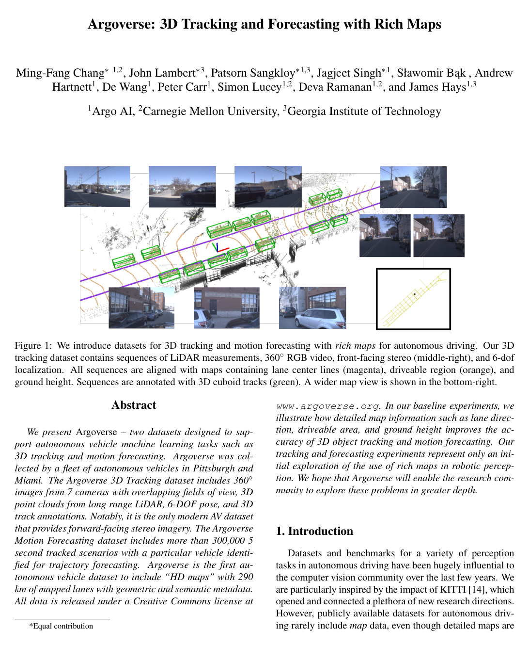
Argoverse: 3D Tracking and Forecasting With Rich Maps

Ming-Fang ChangJohn LambertPatsorn SangkloyJagjeet SinghSlawomir BakAndrew HartnettDe WangPeter CarrSimon LuceyDeva Ramanan

article2019CVPR1,673 citations

Introduces a pioneering autonomous driving benchmark that pairs sensor data and stereo imagery with high-definition geometric and semantic maps to advance 3D tracking and motion forecasting.

Listen

Autonomous vehicle perception systems require accurate spatial context to safely navigate complex urban environments, yet publicly available benchmarks have historically lacked rich geometric and semantic map data. This limitation has hindered research into how detailed prior map knowledge can assist onboard sensor systems in tasks such as object tracking and path prediction.

The article introduces Argoverse, a large-scale open-source dataset, and evaluates how incorporating high-definition map features directly impacts the accuracy of 3D object tracking and motion forecasting algorithms.

The researchers collected real-world sensor data across Pittsburgh and Miami using autonomous vehicle fleets equipped with long-range LiDAR, 360-degree cameras, and stereo imagery. The resulting benchmark pairs these sensor streams with rich map layers, including 290 linear kilometers of lane centerlines with semantic connectivity, a digital ground height model, and binary driveable area coverage. The dataset features 113 human-annotated vehicle log segments for 3D tracking across 15 object classes and over 324,000 mined five-second scenarios capturing challenging driving maneuvers for trajectory forecasting.

The evaluation established several core findings. First, integrating vector map lane directions substantially improved vehicle orientation estimation during 3D tracking, cutting orientation error nearly in half from roughly 25–28 degrees to 13–15 degrees across near and far ranges. Second, using high-definition maps for ground-point filtering maintained steady 3D bounding box shape accuracy and improved object detection scores compared to traditional planar ground-fitting heuristics, particularly in sloped and uneven terrain. Third, baseline tracking accuracy degraded sharply with distance, dropping from a Multi-Object Tracking Accuracy score of 65.5% within 30 meters down to 34.2% within 100 meters due to sensor point sparsity. Finally, in motion forecasting, leveraging map centerlines as reference priors and using driveable area boundaries to prune invalid paths produced multi-path trajectory forecasts with drivable area compliance rates as high as 94% to 99%.

These findings demonstrate that detailed map priors serve as critical computational aids for perception systems. Incorporating semantic road infrastructure directly addresses false detections and physical violations, enhancing safety and route-planning reliability while reducing onboard real-time processing burdens. The results show that even simple statistical models utilizing map priors can outperform complex, unconstrained machine learning models by restricting predicted behaviors to physically plausible road lanes.

Autonomous driving engineering teams and researchers should adopt multimodal datasets that integrate high-definition vector maps to train perception models. Future technical efforts should prioritize developing advanced machine learning models that jointly leverage camera, LiDAR, and map representations, alongside building automated mapping systems to scale these annotations to new geographic regions.

While the dataset offers substantial scale and diversity, the motion forecasting scenarios rely on automatically mined trajectories from fleet operations, which introduces a degree of label noise compared to manually certified ground truth. Readers should exercise caution when evaluating long-range tracking capabilities, as LiDAR point sparsity beyond 50 meters remains a fundamental hardware constraint.

Argo AI Carnegie Mellon University Georgia Institute of Technology http object tracking point cloud Argoverse dataset 3D tracking motion forecasting

arXiv: 1911.02620 argoverse/argoverse-api

Paper: PointRCNN: 3D Object Proposal Generation and Detection From Point Cloud, Shaoshuai Shi et al. (2019). Argoverse's 3D tracking and detection tasks directly rely on foundational 3D proposal generation architectures like PointRCNN that operate on raw LiDAR point clouds.
Paper: Multi-view 3D Object Detection Network for Autonomous Driving, Xiaozhi Chen et al. (2017). Argoverse evaluates multi-sensor 3D perception baselines that build on multi-view fusion architectures combining LiDAR point clouds and camera imagery pioneered by MV3D.
Paper: MOT16: A Benchmark for Multi-Object Tracking, Anton Milan et al. (2016). Argoverse adapts standardized multi-object tracking metrics and benchmark evaluation formulations established by benchmarks like MOT16 to the 3D domain.
Paper: The Cityscapes Dataset for Semantic Urban Scene Understanding, Marius Cordts et al. (2016). Cityscapes established the paradigm of large-scale, multi-city urban datasets for autonomous vehicle scene understanding that Argoverse expands with LiDAR and HD maps.
Paper: Object scene flow for autonomous vehicles, Moritz Menze et al. (2015). Menze and Geiger established foundational principles and dynamic scene benchmarks for multi-object 3D motion estimation from stereo imagery in autonomous driving.

Paper: Lift, Splat, Shoot: Encoding Images From Arbitrary Camera Rigs by Implicitly Unprojecting to 3D, Jonah Philion et al. (2020). Lift, Splat, Shoot builds upon modern multi-camera autonomous driving benchmark suites like Argoverse to learn unified bird's-eye-view representations for downstream planning and forecasting.
Paper: BEVFormer: Learning Bird's-Eye-View Representation from Multi-Camera Images via Spatiotemporal Transformers, Zhiqi Li et al. (2022). BEVFormer advances the multi-camera 3D detection and tracking problems framed by Argoverse by incorporating spatiotemporal transformers in bird's-eye view.
Paper: BEVFusion: Multi-Task Multi-Sensor Fusion with Unified Bird's-Eye View Representation, Zhijian Liu et al. (2022). BEVFusion extends multi-sensor 3D perception on urban AV datasets by developing an optimized shared bird's-eye-view representation for LiDAR and camera fusion.
Paper: Center-based 3D Object Detection and Tracking, Tianwei Yin et al. (2020). CenterPoint introduces point-centered 3D detection and velocity-based tracking methods tailored to large-scale urban driving benchmarks.
Paper: BDD100K: A Diverse Driving Dataset for Heterogeneous Multitask Learning, Fisher Yu et al. (2020). BDD100K expands the scale and multi-task scope of driving benchmarks beyond the tracking and trajectory forecasting tasks featured in Argoverse.
Paper: Adaptive Graph Convolutional Recurrent Network for Traffic Forecasting, Lei Bai et al. (2020). Adaptive Graph Convolutional Recurrent Network builds on the spatio-temporal road graph forecasting challenges introduced in autonomous driving datasets.

Cover for Argoverse: 3D Tracking and Forecasting With Rich Maps

Abstract

We present Argoverse -- two datasets designed to support autonomous vehicle machine learning tasks such as 3D tracking and motion forecasting. Argoverse was collected by a fleet of autonomous vehicles in Pittsburgh and Miami. The Argoverse 3D Tracking dataset includes 360 degree images from 7 cameras with overlapping fields of view, 3D point clouds from long range LiDAR, 6-DOF pose, and 3D track annotations. Notably, it is the only modern AV dataset that provides forward-facing stereo imagery. The Argoverse Motion Forecasting dataset includes more than 300,000 5-second tracked scenarios with a particular vehicle identified for trajectory forecasting. Argoverse is the first autonomous vehicle dataset to include "HD maps" with 290 km of mapped lanes with geometric and semantic metadata. All data is released under a Creative Commons license at this http URL. In our baseline experiments, we illustrate how detailed map information such as lane direction, driveable area, and ground height improves the accuracy of 3D object tracking and motion forecasting. Our tracking and forecasting experiments represent only an initial exploration of the use of rich maps in robotic perception. We hope that Argoverse will enable the research community to explore these problems in greater depth.

Topics

http object tracking point cloud self-driving auto semantic metadata autonomous robot

Keywords

Argoverse dataset 3D tracking motion forecasting trajectory prediction rich maps autonomous driving datasets point cloud

1 Introduction
2 Related Work
3 The Argoverse Dataset
3.1 Maps
3.2 3D Track Annotations
3.3 Mined Trajectories for Motion Forecasting
4 3D Object Tracking
4.1 Evaluation
5 Motion Forecasting
5.1 Problem Description
5.2 Evaluation of Multiple Forecasts
5.3 Results
6 Discussion
References
A Supplemental Map Details
A.1 Coordinate System
A.2 Map API and Software Development Kit
B 3D Tracking Taxonomy Details
C Supplemental Details on Motion Forecasting
C.1 Motion Forecasting Data Mining Details
C.2 2D Curvilinear Centerline Coordinate System
D Supplemental Tracking Details
D.1 Tracker Implementation Details
D.2 Tracking Evaluation Metrics
D.3 True Positive Thresholding Discussion

Knowls

Knowl 1 — Argoverse Autonomous Driving Dataset Suite
experimental setup
The Argoverse dataset comprises two distinct benchmarks collected by autonomous vehicle fleets operating in Pittsburgh, Pennsylvania, and Miami, Florida:
1. Argoverse 3D Tracking Dataset: Contains 113 human-annotated vehicle log sequences ranging between 15 and 30 seconds in duration (65 train, 24 validation, and 24 test logs), containing 11,052 distinct tracked 3D objects across 15 semantic classes annotated within 5 meters of the drivable road area. Sensor streams include:
  - Two roof-mounted, rotating 32-beam LiDAR sensors capturing at 10 Hz out-of-phase (40° vertical field of view each, 30° vertical overlap, 50° combined vertical field of view, range up to 200 m, and ~107,000 motion-compensated 3D points per combined sweep).
  - Seven high-resolution ring cameras ( $1920 \times 1200$ pixels) operating at 30 Hz providing 360° visual coverage.
  - Two front-facing stereo cameras ( $2056 \times 2464$ pixels) operating at 5 Hz with a baseline of 0.2986 m.
  - 6-DOF ego-vehicle pose localized within city coordinates.
2. Argoverse Motion Forecasting Dataset: Contains 324,557 five-second scenarios (205,942 train, 39,472 validation, and 78,143 test sequences) sampled at 10 Hz mined from 1,006 driving hours. Each sequence includes 2D bird's-eye-view centroid tracks for all observed dynamic objects and designates a single vehicle executing an active maneuver as the focal prediction target.
Knowl 2 — Argoverse HD Vector and Raster Map Architecture
definition
The Argoverse High-Definition (HD) Map provides geometric and semantic priors organized into three complementary representations:
1. Vector Map of Lane Geometry: A directed graph where each lane segment is represented by a 3D polyline centerline composed of ordered vertex pairs $((x_i, y_i, z_i), (x_{i+1}, y_{i+1}, z_{i+1}))$ . Semantic attributes associated with each lane segment include predecessor IDs, successor IDs (enabling branching and merging graph traversal), turn direction (left, right, or none), and Boolean flags is_intersection and has_traffic_control. Mapped lanes cover 204 linear kilometers in Miami (mean drivable lane width $3.84 \pm 0.89$ m) and 86 linear kilometers in Pittsburgh (mean drivable lane width $3.97 \pm 1.04$ m).
2. Rasterized Ground Height Map: A 1-meter grid resolution raster map specifying real-valued terrain elevation above sea level in city coordinates, enabling accurate ground point removal on slopes and non-planar terrain.
3. Rasterized Driveable Area and Region of Interest (ROI): A 1-meter grid resolution binary raster map defining regions where vehicles can physically drive ( $788,510\text{ m}^2$ in Miami; $286,104\text{ m}^2$ in Pittsburgh). The Region of Interest (ROI) is defined as the drivable area expanded by a 5-meter buffer.
Coordinates are expressed in local tangent plane city frames centered at UTM Zone 17 origins:
- Pittsburgh: $(583710.0070\text{ m Easting}, 4477259.9999\text{ m Northing})$
- Miami: $(580560.0088\text{ m Easting}, 2850959.9999\text{ m Northing})$
Points in the ego-vehicle coordinate system ( $p_{\text{egovehicle}}$ ) are transformed to the city frame ( $p_{\text{city}}$ ) via:

$p_{\text{city}} = {}^{\text{city}}T_{\text{egovehicle}} \, p_{\text{egovehicle}}$
Knowl 3 — Motion Forecasting Problem Formulation and Evaluation Metrics
equation
In the motion forecasting setting, given an observed 2D trajectory of a target vehicle $X_i = (x_i^t, y_i^t)_{t=1}^{T_{\text{obs}}}$ for $T_{\text{obs}} = 20$ timesteps (2.0 seconds at 10 Hz), a model generates $K$ candidate future trajectory predictions $\{\hat{Y}_i^{(k)}\}_{k=1}^K$ , where each prediction is $\hat{Y}_i^{(k)} = (\hat{x}_i^t, \hat{y}_i^t)_{t=T_{\text{obs}}+1}^{T_{\text{pred}}}$ for $T_{\text{pred}} = 50$ timesteps (3.0 seconds into the future). Performance is evaluated over the test set using the following metrics for $K \in \{1, 3, 6, 9\}$ :
- Minimum Final Displacement Error (minFDE): Euclidean distance between the ground truth endpoint and the predicted endpoint of the single closest candidate trajectory:
$\text{minFDE} = \min_{k \in \{1, \dots, K\}} \|\hat{Y}_i^{(k)}(T_{\text{pred}}) - Y_i(T_{\text{pred}})\|_2$
- Minimum Average Displacement Error (minADE): Average displacement error computed along the candidate trajectory $k^*$ that minimizes the final displacement error:
$\text{minADE} = \frac{1}{T_{\text{pred}} - T_{\text{obs}}} \sum_{t=T_{\text{obs}}+1}^{T_{\text{pred}}} \|\hat{Y}_i^{(k^*)}(t) - Y_i(t)\|_2, \quad \text{where } k^* = \arg\min_{k \in \{1, \dots, K\}} \|\hat{Y}_i^{(k)}(T_{\text{pred}}) - Y_i(T_{\text{pred}})\|_2$
- Drivable Area Compliance (DAC): The proportion of all $n$ generated future trajectories across test instances that remain entirely inside the map-defined drivable area polygon throughout the prediction horizon, where $m$ denotes trajectories that exit the drivable area at any timestep:
$\text{DAC} = \frac{n - m}{n}$
- Miss Rate (MR): The fraction of test scenarios where the final predicted position of the best candidate trajectory ( $k^*$ ) is greater than 2.0 meters away from the ground truth destination ( $m$ misses out of $n$ evaluation samples):
$\text{MR} = \frac{m}{n}$

Knowl 4 — Motion Forecasting Benchmark Baseline Results

data/table

The motion forecasting benchmark compares deterministic models ( $K=1$ ) and multi-hypothesis predictors ( $K=3, 6$ ) using social interaction features and HD map priors over a 3-second forecasting horizon:

	$K=1$				$K=3$				$K=6$
Model	minADE $\downarrow$	minFDE $\downarrow$	DAC $\uparrow$	MR $\downarrow$	minADE $\downarrow$	minFDE $\downarrow$	DAC $\uparrow$	MR $\downarrow$	minADE $\downarrow$	minFDE $\downarrow$	DAC $\uparrow$	MR $\downarrow$
Constant Velocity	3.53	7.89	0.88	0.83	-	-	-	-	-	-	-	-
NN	3.45	7.88	0.87	0.87	2.16	4.53	0.87	0.70	1.71	3.29	0.87	0.54
LSTM	2.15	4.97	0.93	0.75	-	-	-	-	-	-	-	-
LSTM+social	2.15	4.95	0.93	0.75	-	-	-	-	-	-	-	-
NN+map(prune)	3.38	7.62	0.99	0.86	2.11	4.36	0.97	0.68	1.68	3.19	0.94	0.52
NN+map(prior) $m$ -G, $n$ -C	3.65	8.12	0.83	0.94	2.46	5.06	0.97	0.63	2.08	4.02	0.96	0.58
NN+map(prior) 1-G, $n$ -C	3.65	8.12	0.83	0.94	3.01	6.43	0.95	0.80	2.60	5.32	0.92	0.75
LSTM+map(prior) 1-G, $n$ -C	2.92	6.45	0.98	0.75	2.31	4.85	0.97	0.71	2.08	4.19	0.95	0.67

Key takeaways from these results:

For single predictions ( $K=1$ ), LSTM networks learn temporal trajectory dynamics better than Nearest Neighbor (NN) lookups, achieving $\text{minADE} = 2.15\text{ m}$ vs $3.45\text{ m}$ .
Using vector map centerlines as coordinate reference frames (map(prior)) significantly increases Drivable Area Compliance (DAC reaches up to 0.98 for LSTM and 0.99 for NN with map pruning).
Pruning nearest-neighbor predictions with the drivable area map (NN+map(prune)) achieves the lowest error among all evaluated models at $K=6$ ( $\text{minADE} = 1.68\text{ m}$ , $\text{minFDE} = 3.19\text{ m}$ , $\text{MR} = 0.52$ ).
Allowing multiple speed/acceleration guesses along fewer candidate centerlines (NN+map(prior) m-G,n-C) substantially outperforms taking only one guess per centerline (NN+map(prior) 1-G,n-C), reducing minFDE from 5.32 m to 4.02 m at $K=6$ .

Knowl 5 — Argoverse Baseline 3D Object Tracking Pipeline
algorithm
The Argoverse 3D multi-object tracking baseline combines LiDAR point cloud clustering, 2D image semantic segmentation, and map heuristics to track vehicles in 3D space:
Input: Sequence of synchronized LiDAR point clouds $P_t \subset \mathbb{R}^3$ and 7-ring camera images $I_t$ , vector and raster HD maps
Output: 3D bounding cuboid tracks $\{T_j\}$ with 6-DOF poses, orientations, and velocities
for each timestamp $t = 1, \dots, F$ do
    // 1. Segmentation and Detection
    Filter $P_t$ to points within the map-defined driveable area
    Remove ground points (points within 30 cm of ground surface via ground height map)
    Cluster remaining 3D points using DBSCAN into distinct spatial clusters
    Compute 2D vehicle instance masks on camera images $I_t$ using Mask R-CNN
    Discard LiDAR clusters whose perspective camera projections fall outside vehicle masks
    Filter clusters violating standard car bounding dimensions
    Estimate cluster 3D centroid by fitting a minimum enclosing circle over horizontal coordinates
    // 2. Data Association
    Compute pairwise Euclidean centroid distances between active tracks and current detections
    Solve global optimal assignment via the Hungarian algorithm with gating threshold = 2.0 m
    for each unmatched active track do
        Propagate track pose using a constant-velocity Kalman filter motion model (up to 5 frames)
        if unmatched frames > 5 then terminate track
    for each unassigned cluster detection do
        Initialize a new track ID with a predefined bounding box dimension
    // 3. Pose Estimation and Map Refinement
    for each matched track do
        Estimate relative frame-to-frame rigid transformation using Iterative Closest Point (ICP)
        Update 6-DOF pose and linear velocity state using the Kalman filter measurement update
        if track contains sparse LiDAR points and is not inside an intersection then
            Snap bounding box yaw orientation to the vector map lane centerline tangent direction

Knowl 6 — Argoverse 3D Tracking Accuracy and Map Feature Ablation

data/table

The Argoverse tracking baseline evaluated on the 24-log test set demonstrates tracking performance across evaluation range thresholds and isolates the contribution of map ground removal and map lane direction orientation snapping:

Range	MOTA	MOTP-D (m)	MOTP-O ( $^\circ$ )	MOTP-I	IDF1	MT(%)	ML(%)	#FP	#FN	IDSW	#FRAG
$\le 30$ m	65.5	0.71	15.3	0.25	0.71	0.67	0.18	5739	10098	356	380
$\le 50$ m	50.0	0.81	13.5	0.26	0.59	0.30	0.31	8191	30468	607	691
$\le 100$ m	34.2	0.82	13.3	0.25	0.46	0.13	0.51	9225	66234	679	773

Tracking accuracy diminishes sharply as distance increases past 50 m due to lower LiDAR point density, with Mostly Tracked (MT) trajectories dropping from 67% to 13% and False Negatives (FN) increasing sixfold.

Ablation over map features across distances:

Range	Use Map Lane	Ground Removal	MOTA	MOTP-D (m)	MOTP-O ( $^\circ$ )	MOTP-I
30 m	Yes	Map Height	65.5	0.71	15.3	0.25
30 m	Yes	Plane-Fitting	65.8	0.72	13.7	0.29
30 m	No	Map Height	65.4	0.71	25.3	0.25
50 m	Yes	Map Height	50.0	0.81	13.5	0.26
50 m	Yes	Plane-Fitting	49.3	0.81	12.5	0.29
50 m	No	Map Height	49.8	0.81	27.7	0.26
100 m	Yes	Map Height	34.2	0.82	13.3	0.25
100 m	Yes	Plane-Fitting	33.6	0.82	12.5	0.28
100 m	No	Map Height	34.1	0.82	27.7	0.25

Using HD map ground height improves box shape precision (MOTP-I error reduced from 0.28–0.29 down to 0.25–0.26) and long-range MOTA over naive planar ground fitting.
Snapping bounding box yaw to map lane directions reduces vehicle orientation error (MOTP-O) by approximately $10^\circ$ to $14^\circ$ across all distance ranges.

Knowl 7 — 3D Tracking Evaluation Metrics and Centroid Distance Thresholding
definition
Argoverse evaluates 3D multi-object tracking using standard MOT metrics adapted for 3D autonomous vehicle perception:
- Multi-Object Tracking Accuracy (MOTA): Measures detection and association accuracy:
$\text{MOTA} = 100 \times \left( 1 - \frac{\sum_t (\text{FN}_t + \text{FP}_t + \text{IDsw}_t)}{\sum_t \text{GT}_t} \right)$

where $\text{FN}_t$ , $\text{FP}_t$ , $\text{IDsw}_t$ , and $\text{GT}_t$ represent the counts of false negatives, false positives, identity switches, and ground truth objects at timestep $t$ .
- Multi-Object Tracking Precision (MOTP): Assesses geometric precision across matched ground truth and prediction pairs:
$\text{MOTP} = \frac{\sum_{i,t} D_t^i}{\sum_t C_t}$

where $C_t$ is the number of matched pairs at time $t$ and $D_t^i$ is the match error under one of three distances:
1. MOTP-D (Centroid Distance): Euclidean distance between 3D bounding box centers.
2. MOTP-O (Orientation Error): Smallest angular yaw difference about the vertical $z$ -axis (ignoring front/back disambiguation).
3. MOTP-I (Amodal Shape Error): $1 - \text{IoU}$ of the 3D bounding boxes after translating centroids and rotating orientations into alignment.
- IDF1: The harmonic mean of identification precision and identification recall based on global identity assignments.
True Positive Assignment Thresholding: Associations between tracker predictions and ground truth annotations are determined using a fixed absolute 3D centroid distance threshold of 2.0 meters (half the length of a standard passenger vehicle) rather than an Intersection-over-Union (IoU) threshold. Fixed 3D distance thresholding prevents smaller object classes (e.g., pedestrians) from being penalized orders of magnitude more severely than large objects (e.g., buses) for identical spatial localization errors, and accommodates sparse LiDAR point clouds at long range.
Knowl 8 — Trajectory Coordinate Normalization and Curvilinear Lane Transformations
model/method
To enhance model generalizability across arbitrary map positions and road geometries, trajectory coordinates are mapped into normalized reference frames:
1. Unmapped Trajectory Normalization: For models operating without HD maps, observed 2D Cartesian trajectory coordinates $(x_i^t, y_i^t)$ for $t = 1, \dots, T_{\text{obs}}$ are translated and rotated such that the initial observation begins at the origin $(x_i^1, y_i^1) = (0, 0)$ and the final observed position $(x_i^{T_{\text{obs}}}, y_i^{T_{\text{obs}}})$ lies on the positive $x$ -axis, satisfying $y_i^{T_{\text{obs}}} = 0$ with $x_i^{T_{\text{obs}}} > 0$ .
2. 2D Curvilinear Centerline Coordinate System: For map-conditioned models, a vehicle's Cartesian coordinates $(x_i^t, y_i^t)$ are projected onto the nearest lane centerline polyline from the vector map and represented as:
  - $a_i^t$ : The along-track longitudinal distance traveled along the centerline from the start of the lane segment.
  - $o_i^t$ : The cross-track lateral offset perpendicular to the centerline tangent.
Trajectories predicted in curvilinear coordinates $(a_i^t, o_i^t)$ are transformed back into absolute Cartesian city coordinates $(x_i^t, y_i^t)$ for evaluation against ground truth.
Knowl 9 — Trajectory Mining Strategy for Motion Forecasting Scenarios
model/method
To prevent motion forecasting datasets from being dominated by trivial trajectories (e.g., parked cars or constant-velocity cruising on straight roads), Argoverse employs an automated mining pipeline across 1,006 driving hours to identify rare and safety-critical vehicle maneuvers:
1. For every 5-second window sampled at 10 Hz, an interestingness score is calculated for every object track based on:
  - Position inside an intersection (with or without active traffic control).
  - Presence in designated left-turn or right-turn lanes.
  - Execution of lane change maneuvers to adjacent left or right lane segments.
  - High median velocity or high velocity variance.
  - Visibility duration across the entire 5-second interval.
2. Turning and lane-changing behaviors receive the highest score weights due to their low natural frequency.
3. A 5-second sequence is selected for inclusion if it contains at least two tracks meeting minimum interestingness thresholds.
4. The track with the maximum interestingness score that remains visible throughout the full 5.0 seconds is designated as the primary Agent to forecast. Consecutive mined sequences share a 2.5-second temporal overlap.
Knowl 10 — Trade-Off Between Centerline Branching and Velocity Multimodality
empirical result
In map-prior trajectory forecasting using candidate lane centerlines (NN+map(prior) m-G,n-C), candidate predictions $K$ are factored into $n$ distinct topological route paths (centerlines) and $m$ velocity profile guesses along each centerline such that $K = m \times n$ :
- At budget $K=6$ , allocating guesses across $n=2$ centerlines with $m=3$ velocity profiles per centerline yields $\text{minFDE} = 4.02\text{ m}$ , whereas allocating $m=1$ guess across $n=6$ distinct centerlines yields $\text{minFDE} = 5.32\text{ m}$ .
- At budget $K=9$ , evaluating $n=3$ centerlines with $m=3$ velocity profiles achieves $\text{minFDE} = 3.6\text{ m}$ , whereas evaluating $n=9$ centerlines with $m=1$ guess per centerline achieves $\text{minFDE} = 8.1\text{ m}$ .
When a sufficient number of high-level topological centerlines ( $n \ge 2$ ) covers the set of plausible routing decisions, allocating multi-hypothesis prediction capacity to diverse speed and acceleration profiles ( $m > 1$ ) along those centerlines yields substantially lower displacement errors than predicting single trajectories along a wider set of centerlines.

Coverage note — No substantial contributed material was omitted. Specific visual diagram figures, standard API boilerplate helper functions, and detailed qualitative taxonomy image galleries were summarized into the respective dataset, map architecture, metric, and algorithm knowls.

References

1.Alexandre Alahi, Kratarth Goel, Vignesh Ramanathan, Alexandre Robicquet, Li Fei-Fei, and Silvio Savarese. Social lstm: Human trajectory prediction in crowded spaces. In The IEEE Conference on Computer Vision and Pattern Recognition (CVPR), 2016.
2.Mykhaylo Andriluka, Stefan Roth, and Bernt Schiele. People-tracking-by-detection and people-detection-bytracking. In The IEEE Conference on Computer Vision and Pattern Recognition (CVPR), 2008.
3.Andrew Bacha, Cheryl Bauman, Ruel Faruque, Michael Fleming, Chris Terwelp, Charles Reinholtz, Dennis Hong, Al Wicks, Thomas Alberi, David Anderson, Stephen Cacciola, Patrick Currier, Aaron Dalton, Jesse Farmer, Jesse Hurdus, Shawn Kimmel, Peter King, Andrew Taylor, David Van Covern, and Mike Webster. Odin: Team victortango's entry in the darpa urban challenge. J. Field Robot., 25(8):467–492, Aug. 2008.
4.Min Bai, Gellért Máttyus, Namdar Homayounfar, Shenlong Wang, Shrinidhi Kowshika Lakshmikanth, and Raquel Urtasun. Deep multi-sensor lane detection. In 2018 IEEE/RSJ International Conference on Intelligent Robots and Systems, IROS 2018, Madrid, Spain, October 1-5, 2018, pages 3102–3109, 2018.
5.Keni Bernardin and Rainer Stiefelhagen. Evaluating multiple object tracking performance: The clear mot metrics. EURASIP J. Image and Video Processing, 2008.
6.Holger Caesar, Varun Bankiti, Alex H. Lang, Sourabh Vora, Venice Erin Liong, Qiang Xu, Anush Krishnan, Yu Pan, Giancarlo Baldan, and Oscar Beijbom. nuscenes: A multimodal dataset for autonomous driving. arXiv preprint arXiv:1903.11027, 2019.
7.Sergio Casas, Wenjie Luo, and Raquel Urtasun. Intentnet: Learning to predict intention from raw sensor data. In Aude Billard, Anca Dragan, Jan Peters, and Jun Morimoto, editors, Proceedings of The 2nd Conference on Robot Learning, volume 87 of Proceedings of Machine Learning Research, pages 947–956. PMLR, 29–31 Oct 2018.
8.Florian Chabot, Mohamed Chaouch, Jaonary Rabarisoa, Céline Teulière, and Thierry Chateau. Deep manta: A coarse-to-fine many-task network for joint 2d and 3d vehicle analysis from monocular image. In IEEE Conference on Computer Vision and Pattern Recognition (CVPR), 2017.
9.Chenyi Chen, Ari Seff, Alain Kornhauser, and Jianxiong Xiao. Deepdriving: Learning affordance for direct perception in autonomous driving. In The IEEE International Conference on Computer Vision (ICCV), 2015.
10.Marius Cordts, Mohamed Omran, Sebastian Ramos, Timo Rehfeld, Markus Enzweiler, Rodrigo Benenson, Uwe Franke, Stefan Roth, and Bernt Schiele. The cityscapes dataset for semantic urban scene understanding. In Proc. of the IEEE Conference on Computer Vision and Pattern Recognition (CVPR), 2016.
11.Nachiket Deo and Mohan M Trivedi. Convolutional social pooling for vehicle trajectory prediction. arXiv preprint arXiv:1805.06771, 2018.
12.Alexey Dosovitskiy, German Ros, Felipe Codevilla, Antonio Lopez, and Vladlen Koltun. Carla: An open urban driving simulator. arXiv preprint arXiv:1711.03938, 2017.
13.Martin Ester, Hans peter Kriegel, Jörg Sander, and Xiaowei Xu. A density-based algorithm for discovering clusters in large spatial databases with noise. In KDD Proceedings of the Second International Conference on Knowledge Discovery and Data Mining, pages 226–231. AAAI Press, 1996.
14.Andreas Geiger, Philip Lenz, Christoph Stiller, and Raquel Urtasun. Vision meets robotics: The KITTI dataset. The International Journal of Robotics Research, 32(11):1231–1237, 2013.
15.Alex Graves. Generating sequences with recurrent neural networks. CoRR, abs/1308.0850, 2013.
16.Junyao Guo, Unmesh Kurup, and Mohak Shah. Is it safe to drive? an overview of factors, challenges, and datasets for driveability assessment in autonomous driving. IEEE Transactions on Intelligent Transportation Systems, 2019.
17.Agrim Gupta, Justin Johnson, Li Fei-Fei, Silvio Savarese, and Alexandre Alahi. Social gan: Socially acceptable trajectories with generative adversarial networks. In The IEEE Conference on Computer Vision and Pattern Recognition (CVPR), June 2018.
18.K. He, G. Gkioxari, P. Dollár, and R. Girshick. Mask r-cnn. In 2017 IEEE International Conference on Computer Vision (ICCV), pages 2980–2988, Oct 2017.
19.Kaiming He, Georgia Gkioxari, Piotr Dollár, and Ross Girshick. Mask R-CNN. In Proceedings of the International Conference on Computer Vision (ICCV), 2017.
20.Simon Hecker, Dengxin Dai, and Luc Van Gool. End-to-end learning of driving models with surround-view cameras and route planners. In European Conference on Computer Vision (ECCV), 2018.
21.David Held, Devin Guillory, Brice Rebsamen, Sebastian Thrun, and Silvio Savarese. A probabilistic framework for real-time 3d segmentation using spatial, temporal, and semantic cues. In Proceedings of Robotics: Science and Systems, 2016.
22.David Held, Jesse Levinson, and Sebastian Thrun. Precision tracking with sparse 3d and dense color 2d data. In ICRA, 2013.
23.David Held, Jesse Levinson, Sebastian Thrun, and Silvio Savarese. Combining 3d shape, color, and motion for robust anytime tracking. In Proceedings of Robotics: Science and Systems, Berkeley, USA, July 2014.
24.Michael Himmelsbach and Hans-Joachim Wünsche. Lidar-based 3d object perception. In Proceedings of 1st International Workshop on Cognition for Technical Systems, 2008.
25.Namdar Homayounfar, Wei-Chiu Ma, Shrinidhi Kowshika Lakshmikanth, and Raquel Urtasun. Hierarchical recurrent attention networks for structured online maps. In The IEEE Conference on Computer Vision and Pattern Recognition (CVPR), June 2018.
26.Xinyu Huang, Xinjing Cheng, Qichuan Geng, Binbin Cao, Dingfu Zhou, Peng Wang, Yuanqing Lin, and Ruigang Yang. The apolloscape dataset for autonomous driving. In arXiv:1803.06184, 2018.
27.Simon Julier, Jeffrey Uhlmann, and Hugh F Durrant-Whyte. A new method for the nonlinear transformation of means and covariances in filters and estimators. IEEE Transactions on automatic control, 45(3):477–482, 2000.
28.Simon J Julier, Jeffrey K Uhlmann, and Hugh F Durrant-Whyte. A new approach for filtering nonlinear systems. In Proceedings of 1995 American Control Conference-ACC’95, volume 3, pages 1628–1632. IEEE, 1995.
29.R. Kesten, M. Usman, J. Houston, T. Pandya, K. Nadhamuni, A. Ferreira, M. Yuan, B. Low, A. Jain, P. Ondruska, S. Omari, S. Shah, A. Kulkarni, A. Kazakova, C. Tao, L. Platinsky, W. Jiang, and V. Shet. Lyft level 5 av dataset 2019. https://level5.lyft.com/dataset/, 2019.
30.Abhijit Kundu, Yin Li, and James M. Rehg. 3d-rcnn: Instance-level 3d object reconstruction via render-and-compare. In IEEE Conference on Computer Vision and Pattern Recognition (CVPR), 2018.
31.Alex H. Lang, Sourabh Vora, Holger Caesar, Lubing Zhou, Jiong Yang, and Oscar Beijbom. Pointpillars: Fast encoders for object detection from point clouds. In CVPR, 2018.
32.Namhoon Lee, Wongun Choi, Paul Vernaza, Christopher Bongsoo Choy, Philip H. S. Torr, and Manmohan Krishna Chandraker. DESIRE: distant future prediction in dynamic scenes with interacting agents. CoRR, abs/1704.04394, 2017.
33.John Leonard, Jonathan How, Seth Teller, Mitch Berger, Stefan Campbell, Gaston Fiore, Luke Fletcher, Emilio Frazzoli, Albert Huang, Sertac Karaman, Olivier Koch, Yoshiaki Kuwata, David Moore, Edwin Olson, Steve Peters, Justin Teo, Robert Truax, Matthew Walter, David Barrett, Alexander Epstein, Keoni Maheloni, Katy Moyer, Troy Jones, Ryan Buckley, Matthew Antone, Robert Galejs, Siddhartha Krishnamurthy, and Jonathan Williams. A perception-driven autonomous urban vehicle. J. Field Robot., 25(10):727–774, Oct. 2008.
34.Jesse Levinson, Jake Askeland, Jan Becker, Jennifer Dolson, David Held, Sören Kammel, J. Zico Kolter, Dirk Langer, Oliver Pink, Vaughan R. Pratt, Michael Sokolsky, Ganymed Stanek, David Michael Stavens, Alex Teichman, Moritz Werling, and Sebastian Thrun. Towards fully autonomous driving: Systems and algorithms. In IEEE Intelligent Vehicles Symposium (IV), 2011, Baden-Baden, Germany, June 5-9, 2011, pages 163–168, 2011.
35.Justin Liang, Namdar Homayounfar, Wei-Chiu Ma, Shenlong Wang, and Raquel Urtasun. Convolutional recurrent network for road boundary extraction. In The IEEE Conference on Computer Vision and Pattern Recognition (CVPR), June 2019.
36.Justin Liang and Raquel Urtasun. End-to-end deep structured models for drawing crosswalks. In The European Conference on Computer Vision (ECCV), September 2018.
37.Ming Liang, Bin Yang, Yun Chen, Rui Hu, and Raquel Urtasun. Multi-task multi-sensor fusion for 3d object detection. In The IEEE Conference on Computer Vision and Pattern Recognition (CVPR), June 2019.
38.Xingyu Liu, Charles R Qi, and Leonidas J Guibas. Flownet3d: Learning scene flow in 3d point clouds. arXiv preprint arXiv:1806.01411, 2019.
39.Wenjie Luo, Bin Yang, and Raquel Urtasun. Fast and furious: Real time end-to-end 3d detection, tracking and motion forecasting with a single convolutional net. In The IEEE Conference on Computer Vision and Pattern Recognition (CVPR), June 2018.
40.Suraj M S, Hugo Grimmett, Lukas Platinsky, and Peter Ondruska. Visual vehicle tracking through noise and occlusions using crowd-sourced maps. In Intelligent Robots and Systems (IROS), 2018 IEEE international conference on, pages 4531–4538. IEEE, 2018.
41.Yuexin Ma, Xinge Zhu, Sibo Zhang, Ruigang Yang, Wenping Wang, and Dinesh Manocha. Trafficpredict: Trajectory prediction for heterogeneous traffic-agents. In Proceedings of the 33rd National Conference on Artifical Intelligence, AAAI’19. AAAI Press, 2019.
42.Will Maddern, Geoffrey Pascoe, Chris Linegar, and Paul Newman. 1 year, 1000 km: The Oxford Robotcar dataset. The International Journal of Robotics Research, 36(1):3–15, 2017.
43.A. Milan, L. Leal-Taixé, I. Reid, S. Roth, and K. Schindler. MOT16: A benchmark for multi-object tracking. arXiv:1603.00831 [cs], Mar. 2016. arXiv: 1603.00831.
44.Michael Montemerlo, Jan Becker, Suhrid Bhat, Hendrik Dahlkamp, Dmitri Dolgov, Scott Ettinger, Dirk Haehnel, Tim Hilden, Gabe Hoffmann, Burkhard Huhnke, Doug Johnston, Stefan Klumpp, Dirk Langer, Anthony Levandowski, Jesse Levinson, Julien Marcil, David Orenstein, Johannes Paefgen, Isaac Penny, Anna Petrovskaya, Mike Pflueger, Ganymed Stanek, David Stavens, Antone Vogt, and Sebastian Thrun. Junior: The stanford entry in the urban challenge. J. Field Robot., 25(9):569–597, Sept. 2008.
45.Gaurav Pandey, James R Mcbride, and Ryan M Eustice. Ford campus vision and lidar data set. Int. J. Rob. Res., 30(13):1543–1552, Nov. 2011.
46.SeongHyeon Park, Byeongdo Kim, Chang Mook Kang, Chung Choo Chung, and Jun Won Choi. Sequence-to-sequence prediction of vehicle trajectory via LSTM encoder-decoder architecture. In Intelligent Vehicles Symposium, pages 1672–1678. IEEE, 2018.
47.Abhishek Patil, Srikanth Malla, Haiming Gang, and Yi-Ting Chen. The h3d dataset for full-surround 3d multi-object detection and tracking in crowded urban scenes. In International Conference on Robotics and Automation, 2019.
48.Luis Patino, Tom Cane, Alain Vallee, and James Ferryman. Pets 2016: Dataset and challenge. In Proceedings of the IEEE Conference on Computer Vision and Pattern Recognition Workshops, pages 1–8, 2016.
49.Akshay Rangesh, Kevan Yuen, Ravi Kumar Satzoda, Rakesh Nattoji Rajaram, Pujitha Gunaratne, and Mohan M. Trivedi. A multimodal, full-surround vehicular testbed for naturalistic studies and benchmarking: Design, calibration and deployment. CoRR, abs/1709.07502, 2017.
50.Nicholas Rhinehart, Kris M Kitani, and Paul Vernaza. R2p2: A reparameterized pushforward policy for diverse, precise generative path forecasting. In Proceedings of the European Conference on Computer Vision (ECCV), pages 772–788, 2018.
51.Nicholas Rhinehart, Rowan McAllister, Kris Kitani, and Sergey Levine. Precog: Prediction conditioned on goals in visual multi-agent settings. arXiv preprint arXiv:1905.01296, 2019.
52.Stephan R. Richter, Zeeshan Hayder, and Vladlen Koltun. Playing for benchmarks. In IEEE International Conference on Computer Vision, ICCV 2017, Venice, Italy, October 22-29, 2017, pages 2232–2241, 2017.
53.R.B. Rusu and S. Cousins. 3d is here: Point cloud library (pcl). In Robotics and Automation (ICRA), 2011 IEEE International Conference on, pages 1 –4, may 2011.
54.John Parr Snyder. Map projections–A working manual, volume 1395, page 61. US Government Printing Office, 1987.
55.Xibin Song, Peng Wang, Dingfu Zhou, Rui Zhu, Chenye Guan, Yuchao Dai, Hao Su, Hongdong Li, and Ruigang Yang. Apollocar3d: A large 3d car instance understanding benchmark for autonomous driving. CoRR, abs/1811.12222, 2018.
56.Ilya Sutskever, Oriol Vinyals, and Quoc V Le. Sequence to sequence learning with neural networks. In Z. Ghahramani, M. Welling, C. Cortes, N. D. Lawrence, and K. Q. Weinberger, editors, Advances in Neural Information Processing Systems 27, pages 3104–3112. Curran Associates, Inc., 2014.
57.Christopher Urmson, Joshua Anhalt, J. Andrew (Drew) Bagnell, Christopher R. Baker, Robert E. Bittner, John M. Dolan, David Duggins, David Ferguson, Tugrul Galatali, Hartmut Geyer, Michele Gittleman, Sam Harbaugh, Martial Hebert, Thomas Howard, Alonzo Kelly, David Kohanbash, Maxim Likhachev, Nick Miller, Kevin Peterson, Raj Rajkumar, Paul Rybski, Bryan Salesky, Sebastian Scherer, Young-Woo Seo, Reid Simmons, Sanjiv Singh, Jarrod M. Snider, Anthony (Tony) Stentz, William (Red) L. Whittaker, and Jason Ziglar. Tartan racing: A multi-modal approach to the darpa urban challenge. Technical report, Carnegie Mellon University, Pittsburgh, PA, April 2007.
58.Shenlong Wang, Min Bai, Gellert Mattyus, Hang Chu, Wenjie Luo, Bin Yang, Justin Liang, Joel Cheverie, Sanja Fidler, and Raquel Urtasun. Torontocity: Seeing the world with a million eyes. In Proceedings of the IEEE Conference on Computer Vision and Pattern Recognition, 2017.
59.Weiyue Wang, Ronald Yu, Qiangui Huang, and Ulrich Neumann. Sgpn: Similarity group proposal network for 3d point cloud instance segmentation. In CVPR, 2018.
60.Bin Yang, Ming Liang, and Raquel Urtasun. Hdnet: Exploiting hd maps for 3d object detection. In Aude Billard, Anca Dragan, Jan Peters, and Jun Morimoto, editors, Proceedings of The 2nd Conference on Robot Learning, volume 87 of Proceedings of Machine Learning Research, pages 146–155. PMLR, 29–31 Oct 2018.
61.Raymond A Yeh, Alexander G Schwing, Jonathan Huang, and Kevin Murphy. Diverse generation for multi-agent sports games. In Proceedings of the IEEE Conference on Computer Vision and Pattern Recognition, pages 4610–4619, 2019.
62.Yin Zhou and Oncel Tuzel. Voxelnet: End-to-end learning for point cloud based 3d object detection. In The IEEE Conference on Computer Vision and Pattern Recognition (CVPR), June 2018.

Citation

MLA

Chang, M.-F., et al. “Argoverse: 3D Tracking and Forecasting With Rich Maps”. 2019 IEEE/CVF Conference on Computer Vision and Pattern Recognition (CVPR), 2019, pp. 8740–49, https://doi.org/10.1109/CVPR.2019.00895.

APA

Chang, M.-F., Lambert, J., Sangkloy, P., Singh, J., Bak, S., Hartnett, A., Wang, D., Carr, P., Lucey, S., Ramanan, D., & Hays, J. (2019). Argoverse: 3D Tracking and Forecasting With Rich Maps. 2019 IEEE/CVF Conference on Computer Vision and Pattern Recognition (CVPR), 8740–8749. https://doi.org/10.1109/CVPR.2019.00895

Chicago

Chang, M.-F., J. Lambert, P. Sangkloy, et al. 2019. “Argoverse: 3D Tracking and Forecasting With Rich Maps”. 2019 IEEE/CVF Conference on Computer Vision and Pattern Recognition (CVPR), 8740–49. https://doi.org/10.1109/CVPR.2019.00895.

Harvard

Chang, M.-F. et al. (2019) “Argoverse: 3D Tracking and Forecasting With Rich Maps”, 2019 IEEE/CVF Conference on Computer Vision and Pattern Recognition (CVPR). IEEE, pp. 8740–8749. Available at: https://doi.org/10.1109/CVPR.2019.00895.

Vancouver

1. Chang M-F, Lambert J, Sangkloy P, et al (2019) Argoverse: 3D Tracking and Forecasting With Rich Maps. In: 2019 IEEE/CVF Conference on Computer Vision and Pattern Recognition (CVPR). IEEE, pp 8740–8749

BibTeX

@inproceedings{Chang_2019, title={Argoverse: 3D Tracking and Forecasting With Rich Maps}, url={http://dx.doi.org/10.1109/CVPR.2019.00895}, DOI={10.1109/cvpr.2019.00895}, booktitle={2019 IEEE/CVF Conference on Computer Vision and Pattern Recognition (CVPR)}, publisher={IEEE}, author={Chang, Ming-Fang and Lambert, John and Sangkloy, Patsorn and Singh, Jagjeet and Bak, Slawomir and Hartnett, Andrew and Wang, De and Carr, Peter and Lucey, Simon and Ramanan, Deva and Hays, James}, year={2019}, month=June, pages={8740–8749} }

Metadata:Crossref

Source Code

This paper has an official code repository available. Click below to access the source code.

View Repository

Access the Paper

This paper is available from its original source. Click below to access the PDF.

Open PDF

License: IEEE

Argoverse: 3D Tracking and Forecasting With Rich Maps

Abstract

Topics

Keywords

Table of Contents

Knowls

Knowl 1 — Argoverse Autonomous Driving Dataset Suite

Knowl 2 — Argoverse HD Vector and Raster Map Architecture

Knowl 3 — Motion Forecasting Problem Formulation and Evaluation Metrics

Knowl 4 — Motion Forecasting Benchmark Baseline Results

Knowl 5 — Argoverse Baseline 3D Object Tracking Pipeline

Knowl 6 — Argoverse 3D Tracking Accuracy and Map Feature Ablation

Knowl 7 — 3D Tracking Evaluation Metrics and Centroid Distance Thresholding

Knowl 8 — Trajectory Coordinate Normalization and Curvilinear Lane Transformations

Knowl 9 — Trajectory Mining Strategy for Motion Forecasting Scenarios

Knowl 10 — Trade-Off Between Centerline Branching and Velocity Multimodality

References

Citation

BibTeX

Source Code

Access the Paper