Object scene flow for autonomous vehicles

Moritz MenzeAndreas Geiger

article2015CVPR2,277 citations

Proposes a discrete-continuous CRF formulation that models dynamic driving scenes as collections of rigidly moving 3D planar superpixels alongside the first realistic 400-scene dynamic benchmark with semi-dense 3D ground truth.

Listen

Autonomous vehicles and mobile robots rely heavily on understanding three-dimensional motion in dynamic environments to ensure obstacle avoidance, navigation, and passenger safety. Estimating this motion—known as 3D scene flow—from stereo cameras is traditionally difficult because existing methods struggle with ambiguous or untextured image regions, and evaluation has been bottlenecked by the absence of realistic benchmarks with moving objects.

The article sets out to demonstrate a novel 3D scene flow model that explicitly structures scenes into a small set of rigidly moving objects and to introduce a realistic, ground-truth dataset of dynamic driving scenes to rigorously evaluate scene flow performance.

To achieve this, the authors formulated a model representing scenes as planar geometric patches (superpixels) linked to a finite set of moving objects and background, optimizing geometric and motion parameters simultaneously using probabilistic inference. To evaluate the model, the authors annotated 400 real-world dynamic driving scenes from the KITTI dataset by combining corrected laser scans for static backgrounds with geometrically precise 3D computer-aided design (CAD) vehicle models fitted to moving objects, creating 200 training and 200 testing scenes with accurate ground truth.

The analysis yielded several key findings. First, the proposed model significantly outperformed all existing baseline methods on the dynamic benchmark, achieving an overall scene flow error rate of 10.63%, compared to 16.85% for the closest competitor (Piecewise Rigid Scene Flow) and over 40% to 67% for traditional methods. Second, the framework proved highly effective at segmenting independently moving foreground objects, cutting foreground scene flow error to 28.76% versus 33.71% for the closest baseline. Third, limiting the scene representation to just five object hypotheses was sufficient to capture real driving environments, confirming that outdoor environments decompose well into a few rigid bodies. Finally, algorithmic optimizations allowed the runtime to drop from 50 minutes to 120 seconds per scene with only a minimal increase in overall error from 10.63% to 11.03%.

These findings indicate that incorporating explicit rigid-object constraints drastically enhances the reliability of 3D motion tracking, reducing collision risks and improving high-level autonomous decision-making. By tying local patches to rigid bodies, the model resolves visual ambiguities that traditionally cause perception pipelines to fail. Furthermore, the newly introduced benchmark provides the autonomous vehicle industry with a realistic standard to assess perception software.

Engineering teams should adopt object-centric scene flow models for perception pipelines to improve motion segmentation and tracking accuracy. Practitioners should also leverage the released 400-scene dataset to benchmark autonomous navigation algorithms. Moving forward, researchers must focus on developing more expressive visual priors to handle remaining edge cases, such as extreme motions near image boundaries and highly reflective or textureless surfaces where current matching techniques degrade.

While confidence in the model's accuracy is high across standard driving scenarios, limitations remain regarding computational speed for real-time deployment and reduced ground-truth precision during extreme displacements exceeding several hundred pixels at image borders. Readers should exercise caution when deploying the framework in non-rigid scenarios (such as tracking pedestrians) or in severe lighting conditions.

Leibniz Universität Hannover Max Planck Institute for Intelligent Systems autonomous driving cad models moving objects Scene Object Motion

Menze et al (2015).pdf

Paper: FlowNet: Learning Optical Flow with Convolutional Networks, Philipp Fischer et al. (2015). FlowNet established the foundational deep learning approach for optical flow regression that later scene flow architectures directly build upon.
Paper: Fully convolutional networks for semantic segmentation, Jonathan Long et al. (2015). Fully convolutional networks introduced end-to-end pixelwise dense prediction paradigms that underpin modern computer vision scene flow systems.

Paper: A Large Dataset to Train Convolutional Networks for Disparity, Optical Flow, and Scene Flow Estimation, Nikolaus Mayer et al. (2016). This work extends object scene flow to end-to-end trainable convolutional neural networks using large-scale synthetic training data.
Paper: PWC-Net: CNNs for Optical Flow Using Pyramid, Warping, and Cost Volume, Deqing Sun et al. (2018). PWC-Net advances optical flow estimation by integrating pyramids, warping, and cost volumes into a compact architecture suitable for autonomous driving.
Paper: RAFT: Recurrent All-Pairs Field Transforms for Optical Flow, Zachary Teed et al. (2020). RAFT builds upon motion estimation formulations by introducing recurrent all-pairs field transforms for superior optical flow accuracy.

Cover for Object scene flow for autonomous vehicles

Abstract

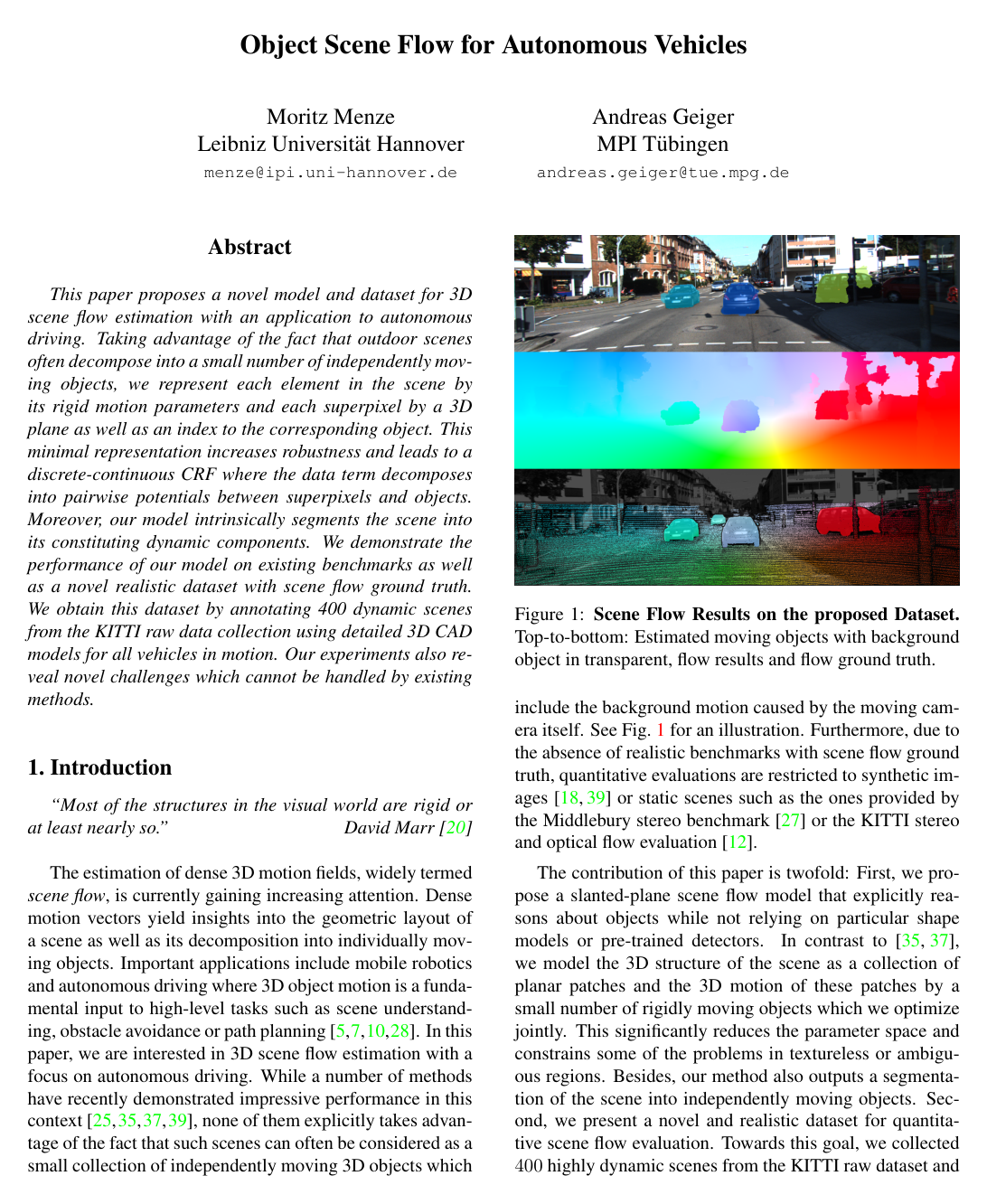
This paper proposes a novel model and dataset for 3D scene flow estimation with an application to autonomous driving. Taking advantage of the fact that outdoor scenes often decompose into a small number of independently moving objects, we represent each element in the scene by its rigid motion parameters and each superpixel by a 3D plane as well as an index to the corresponding object. This minimal representation increases robustness and leads to a discrete-continuous CRF where the data term decomposes into pairwise potentials between superpixels and objects. Moreover, our model intrinsically segments the scene into its constituting dynamic components. We demonstrate the performance of our model on existing benchmarks as well as a novel realistic dataset with scene flow ground truth. We obtain this dataset by annotating 400 dynamic scenes from the KITTI raw data collection using detailed 3D CAD models for all vehicles in motion. Our experiments also reveal novel challenges which cannot be handled by existing methods.

Topics

autonomous driving cad models moving objects real scenes

Keywords

Scene Object Motion Scene Flow Computer Vision Objects Object Scene Flow Stereo Model Ground Truth

1. Introduction
2. Related Work
3. Object Scene Flow
3.1. Data Term
3.2. Smoothness Term
3.3. Inference
4. Scene Flow Dataset and Annotation
4.1. Static Scene Elements
4.2. Moving Objects
5. Experimental Results
6. Conclusion
References

Knowls

Knowl 1 — Object Scene Flow Representation and Energy Formulation
model/method
Object Scene Flow estimates dense 3D geometry and 3D motion from two consecutive stereo image pairs (four calibrated views: left and right at time $t_0$ , and left and right at time $t_1$ ). The reference frame is chosen as the left image at time $t_0$ .

The visual scene is represented as a decomposition into a set of planar superpixel regions $\mathcal{S}$ and a discrete set of rigidly moving 3D objects $\mathcal{O}$ . The static environment ("background") is treated as one of the rigid objects whose motion corresponds to the camera egomotion. Each superpixel $i \in \mathcal{S}$ , covering an image region $R_i$ , is associated with a random variable $s_i = (\mathbf{n}_i, k_i)^T$ , where:
- $\mathbf{n}_i \in \mathbb{R}^3$ specifies the 3D plane equation such that $\mathbf{n}_i^T \mathbf{x} = 1$ for any 3D point $\mathbf{x} \in \mathbb{R}^3$ on the patch in reference coordinates.
- $k_i \in \{1, \ldots, |\mathcal{O}|\}$ is a discrete assignment index identifying the object to which superpixel $i$ belongs.
Each object $j \in \mathcal{O}$ is parameterized by a rigid body transformation $\mathbf{o}_j \in SE(3)$ . A pixel $\mathbf{p}$ inside superpixel $i$ inherits the plane $\mathbf{n}_i$ and the 3D motion $\mathbf{o}_{k_i}$ , which uniquely determines the 3D coordinate and 3D scene flow vector of $\mathbf{p}$ .

The joint state over all superpixels $\mathbf{s} = \{s_i \mid i \in \mathcal{S}\}$ and objects $\mathbf{o} = \{\mathbf{o}_j \mid j \in \mathcal{O}\}$ is inferred by minimizing a discrete-continuous Conditional Random Field (CRF) energy: $E(\mathbf{s}, \mathbf{o}) = \sum_{i \in \mathcal{S}} \phi_i(s_i, \mathbf{o}) + \sum_{i \sim j} \psi_{ij}(s_i, s_j)$ where $\phi_i(s_i, \mathbf{o})$ denotes the data term, $\psi_{ij}(s_i, s_j)$ denotes the pairwise smoothness term, and $i \sim j$ indexes all adjacent superpixel pairs in $\mathcal{S}$ .
Knowl 2 — Multi-View Homography Data Potential with Dense Census and Sparse Matches
model/method
The CRF data potential $\phi_i(s_i, \mathbf{o})$ evaluates photometric consistency by warping pixels from the reference view (left image at $t_0$ ) to the other three images using plane-induced homographies. It decomposes into pairwise potentials between superpixel variables and object hypotheses: $\phi_i(s_i, \mathbf{o}) = \sum_{j \in \mathcal{O}} [k_i = j] \cdot D_i(\mathbf{n}_i, \mathbf{o}_j)$ where $[\cdot]$ is the Iverson bracket, and $D_i(\mathbf{n}, \mathbf{o})$ sums matching costs across the stereo, temporal flow, and cross-stereo views: $D_i(\mathbf{n}, \mathbf{o}) = D^{\text{stereo}}_i(\mathbf{n}, \mathbf{o}) + D^{\text{flow}}_i(\mathbf{n}, \mathbf{o}) + D^{\text{cross}}_i(\mathbf{n}, \mathbf{o})$

For each view $x \in \{\text{stereo}, \text{flow}, \text{cross}\}$ , the matching cost is integrated over all pixels $\mathbf{p} \in R_i$ inside superpixel $i$ : $D^x_i(\mathbf{n}, \mathbf{o}) = \sum_{\mathbf{p} \in R_i} C_x\left(\mathbf{p}, \mathbf{K} \left(\mathbf{R}_x(\mathbf{o}) - \mathbf{t}_x(\mathbf{o}) \mathbf{n}^T\right) \mathbf{K}^{-1} \mathbf{p}\right)$ where $\mathbf{K} \in \mathbb{R}^{3 \times 3}$ is the intrinsic camera calibration matrix, and $[\mathbf{R}_x(\mathbf{o}) \mid \mathbf{t}_x(\mathbf{o})] \in \mathbb{R}^{3 \times 4}$ is the rigid transformation from the reference camera coordinate frame to target frame $x$ under extrinsic calibration and object motion $\mathbf{o}$ .

The matching cost $C_x(\mathbf{p}, \mathbf{q})$ between reference coordinate $\mathbf{p}$ and warped coordinate $\mathbf{q}$ is defined as: $C_x(\mathbf{p}, \mathbf{q}) = \theta_{1,x} C^{\text{dense}}_x(\mathbf{p}, \mathbf{q}) + \theta_{2,x} C^{\text{sparse}}_x(\mathbf{p}, \mathbf{q})$ where:
- $C^{\text{dense}}_x(\mathbf{p}, \mathbf{q})$ is the Hamming distance between $5 \times 5$ Census transform descriptors, truncated at a constant $C_{\text{max}}$ (with pixels outside the target image domain assigned the constant penalty $C_{\text{max}}$ ).
- $C^{\text{sparse}}_x(\mathbf{p}, \mathbf{q}) = \min(\|\boldsymbol{\pi}_x(\mathbf{p}) - \mathbf{q}\|_2, \tau_1)$ if pixel $\mathbf{p}$ belongs to the set of established sparse feature matches $\Pi_x$ , and $0$ otherwise, with $\boldsymbol{\pi}_x(\mathbf{p})$ denoting the sparse correspondence target coordinate and $\tau_1$ a truncation parameter.
Knowl 3 — Geometric and Motion-Boundary Pairwise Smoothness Potentials
model/method
The pairwise smoothness potential $\psi_{ij}(s_i, s_j)$ between adjacent superpixels $i$ and $j$ encourages spatial coherence in depth, surface orientation, and object motion assignments: $\psi_{ij}(s_i, s_j) = \theta_3 \psi^{\text{depth}}_{ij}(\mathbf{n}_i, \mathbf{n}_j) + \theta_4 \psi^{\text{orient}}_{ij}(\mathbf{n}_i, \mathbf{n}_j) + \theta_5 \psi^{\text{motion}}_{ij}(s_i, s_j)$ with weights $\theta_3, \theta_4, \theta_5$ and individual potential components:
1. Depth consistency along the shared boundary $\mathcal{B}_{ij}$ : $\psi^{\text{depth}}_{ij}(\mathbf{n}_i, \mathbf{n}_j) = \sum_{\mathbf{p} \in \mathcal{B}_{ij}} \min(|d(\mathbf{n}_i, \mathbf{p}) - d(\mathbf{n}_j, \mathbf{p})|, \tau_2)$ where $d(\mathbf{n}, \mathbf{p})$ is the disparity of plane $\mathbf{n}$ evaluated at pixel $\mathbf{p}$ , and $\tau_2$ is a truncation threshold.
2. Surface normal orientation smoothness: $\psi^{\text{orient}}_{ij}(\mathbf{n}_i, \mathbf{n}_j) = \min\left(1 - \frac{|\mathbf{n}_i^T \mathbf{n}_j|}{\|\mathbf{n}_i\|_2 \|\mathbf{n}_j\|_2}, \tau_3\right)$ with truncation threshold $\tau_3$ .
3. Motion boundary alignment: $\psi^{\text{motion}}_{ij}(s_i, s_j) = w(\mathbf{n}_i, \mathbf{n}_j) \cdot [k_i \neq k_j]$ where $[\cdot]$ is the Iverson bracket, and the boundary weight $w(\mathbf{n}_i, \mathbf{n}_j)$ is given by: $w(\mathbf{n}_i, \mathbf{n}_j) = \exp\left(-\frac{\lambda}{|\mathcal{B}_{ij}|} \sum_{\mathbf{p} \in \mathcal{B}_{ij}} (d(\mathbf{n}_i, \mathbf{p}) - d(\mathbf{n}_j, \mathbf{p}))^2\right) \cdot \frac{|\mathbf{n}_i^T \mathbf{n}_j|}{\|\mathbf{n}_i\|_2 \|\mathbf{n}_j\|_2}$ with parameter $\lambda$ . This weighting heavily penalizes divergent motion assignments ( $k_i \neq k_j$ ) across coplanar and smooth surfaces while reducing the penalty at 3D geometric folds or depth discontinuities.
Knowl 4 — Ground Truth Annotation for Dynamic Scene Flow via 3D CAD Model Fitting
model/method
Ground truth optical flow and disparity maps for dynamic outdoor driving sequences are generated using a two-stage registration pipeline on multi-frame Velodyne laser scans and stereo images:
1. Static Background Reconstruction: Rolling-shutter distortion in Velodyne scans is corrected using vehicle egomotion and individual laser beam timestamps. Seven consecutive scans are registered into a unified coordinate frame using non-linear least-squares optimization over GPS/IMU poses and Iterative Closest Point (ICP) point cloud alignment. Laser points falling within annotated 3D bounding boxes of moving objects are discarded.
2. Moving Object Registration: For dynamic vehicles, CAD models selected from a database of 16 vehicle types are uniformly sampled into point clouds ( $\sim 3,000$ points each). For each moving object, a 15-dimensional parameter vector $\boldsymbol{\xi} \in \mathbb{R}^{15}$ (specifying 3D pose, scale, and 3D rigid body motion across frames) is estimated by minimizing: $E(\boldsymbol{\xi}) = \sum_{t \in \{1, 2\}} \left( E^{\text{3D}}_t + E^{\text{SGM}}_t + E^{\text{2D}}_t \right)$ where:
- $E^{\text{3D}}_t$ is the average truncated $\ell_2$ distance between 3D laser points in the object bounding box and their nearest points on the CAD model.
- $E^{\text{SGM}}_t$ is the truncated $\ell_1$ distance between CAD model disparity and Semi-Global Matching (SGM) disparity.
- $E^{\text{2D}}_t$ is the squared reprojection error of 5 to 10 manually identified 2D-to-3D keypoint correspondences.
Optimization alternates between non-linear least-squares updates on $\boldsymbol{\xi}$ and updating nearest-neighbor assignments. Densely sampled CAD models are projected into all four camera views using OpenGL z-buffering for occlusion handling. Non-rigid actors (pedestrians, cyclists) are manually masked.
Knowl 5 — Discrete-Continuous Scene Flow Inference via MP-PBP
algorithm
Inference on the discrete-continuous Object Scene Flow CRF is performed using Max-Product Particle Belief Propagation (MP-PBP) with sequential tree-reweighted message passing (TRW-S) for the inner discrete optimization loop.
Input: Four calibrated stereo images, initial superpixels S, max objects |O| = 5, particles per superpixel M_s = 30, particles per object M_o = 10, iterations N_iter = 50
Output: Plane parameters n_i and object assignments k_i for all i in S, rigid motions o_j for all j in O
Initialize superpixels S and initial 3D planes n_i using StereoSLIC
Initialize rigid motions o_j using greedy 3-point RANSAC on sparse scene flow vectors with non-maxima suppression
for iter = 1 to N_iter do
    for each object j in O do
        Sample M_o motion particles from N(o_j^(MAP), Sigma_o)
    end for
    for each superpixel i in S do
        Sample M_s / 2 shape particles from N(n_i^(MAP), Sigma_n)
        Propose M_s / 2 shape particles from plane parameters of spatial neighbors of i
    end for
    Compute data and pairwise potentials over the discrete particle candidate sets
    Solve discrete CRF state assignment using TRW-S
    Update MAP estimates n_i^(MAP), k_i^(MAP) for all i in S, and o_j^(MAP) for all j in O
end for
return {n_i^(MAP), k_i^(MAP)}, {o_j^(MAP)}
A fast variant with $M_s = 10$ , $M_o = 5$ , and $N_{\text{iter}} = 10$ reduces total runtime from 50 minutes to 120 seconds on a 3.0 GHz CPU core.
Knowl 6 — Joint Scene Flow and Disparity Evaluation Metric
definition
The scene flow evaluation metric jointly evaluates the disparity in the reference frame ( $D1$ ), the disparity in the second frame ( $D2$ ), and the 2D optical flow field ( $\mathbf{f} = (u, v)^T$ ).

For a reference view pixel $\mathbf{p}$ with ground truth values $(d_0, d_1, \mathbf{f})$ and estimated values $(\hat{d}_0, \hat{d}_1, \hat{\mathbf{f}})$ , an estimate is flagged as an outlier (error) if its error exceeds 3 pixels and 5% of its true ground truth magnitude:
- $D1$ outlier: $|d_0 - \hat{d}_0| > 3 \text{ px}$ and $|d_0 - \hat{d}_0| / d_0 > 0.05$ .
- $D2$ outlier: $|d_1 - \hat{d}_1| > 3 \text{ px}$ and $|d_1 - \hat{d}_1| / d_1 > 0.05$ , where the second frame disparity is mapped back to the reference frame pixel $\mathbf{p}$ using optical flow with background interpolation.
- Optical flow ( $Fl$ ) outlier: $\|\mathbf{f} - \hat{\mathbf{f}}\|_2 > 3 \text{ px}$ and $\|\mathbf{f} - \hat{\mathbf{f}}\|_2 / \|\mathbf{f}\|_2 > 0.05$ .
- Scene flow ( $SF$ ) outlier: A pixel $\mathbf{p}$ is classified as a scene flow outlier if any of $D1$ , $D2$ , or $Fl$ is an outlier. A pixel is considered correct under $SF$ if and only if all three components are simultaneously accurate.
Error rates are computed as percentage outlier ratios over static background regions (bg), foreground moving objects (fg), and all evaluated pixels (bg+fg).

Knowl 7 — Quantitative Benchmark Evaluation on the KITTI Scene Flow Dataset

data/table

The table below compares Object Scene Flow and several baseline methods on the 200 dynamic test scenes of the annotated KITTI Scene Flow benchmark. Outlier percentages are reported for reference disparity ( $D1$ ), second frame disparity ( $D2$ ), optical flow ( $Fl$ ), and combined scene flow ( $SF$ ), separated into background (bg), foreground (fg), and total pixels (bg+fg).

Method	D1 (%)			D2 (%)			Fl (%)			SF (%)
Method	bg	fg	bg+fg	bg	fg	bg+fg	bg	fg	bg+fg	bg	fg	bg+fg
Huguet et al.	27.31	21.71	26.38	59.51	44.92	57.08	50.06	47.57	49.64	67.69	64.03	67.08
GCSF	11.64	27.11	14.21	32.94	35.76	33.41	47.38	45.07	47.00	52.92	59.11	53.95
SGM + LDOF	5.15	15.27	6.83	29.58	23.47	28.56	41.07	35.52	40.15	43.99	44.77	44.12
SGM + Sun	5.15	15.27	6.83	28.77	25.64	28.25	34.83	45.46	36.60	38.21	53.03	40.68
SGM + Sphere Flow	5.15	15.27	6.83	14.10	23.12	15.60	20.91	28.89	22.24	23.09	37.11	25.42
PRSF	4.74	13.73	6.24	11.14	20.47	12.69	11.73	27.72	14.39	13.49	33.71	16.85
Ours (Fast)	4.45	12.73	5.83	5.41	20.12	7.85	5.71	23.57	8.68	7.14	30.48	11.03
Ours (Full)	4.54	12.03	5.79	5.45	19.41	7.77	5.62	22.18	8.37	7.01	28.76	10.63

Object Scene Flow (Full) achieves a combined scene flow error of $10.63\%$ , outperforming Piecewise Rigid Scene Flow (PRSF) at $16.85\%$ and all modular baselines. Significant improvements are observed in foreground flow ( $22.18\%$ vs. $27.72\%$ for PRSF) and foreground scene flow ( $28.76\%$ vs. $33.71\%$ for PRSF).

Knowl 8 — Ablation of Feature Cues, Pairwise Potentials, and Object Parameterization
empirical result
An ablation study on the 200 test images of the KITTI Scene Flow benchmark isolates the contribution of each model component:
1. Unary Feature Components:
- Dense Census alone yields an overall scene flow ( $SF$ bg+fg) error of $13.96\%$ with unaries only and $10.79\%$ with full pairwise terms.
- Sparse optical flow combined with SGM disparity (SGM+SpF) yields $15.54\%$ with unaries only and $17.03\%$ with full pairwise terms.
- Combining Census and sparse features achieves $13.06\%$ (unaries only) and $10.63\%$ (full model), demonstrating complementary benefits.
1. Pairwise Potentials:
- When added individually to all unaries, the boundary-weighted motion term achieves the largest gain, reducing $SF$ bg+fg error from $13.06\%$ to $11.06\%$ .
- Adding surface normal alignment yields $12.69\%$ , and object identity smoothness yields $12.95\%$ . Combining all pairwise potentials achieves $10.63\%$ .
1. Object Hypothesis Set Size:
- Decreasing the allowed number of object hypotheses $|\mathcal{O}|$ from 5 down to 1 monotonically degrades scene flow accuracy, demonstrating that outdoor scenes cannot be adequately modeled as a single rigidly moving scene.
1. MP-PBP Iterations:
- The MP-PBP optimization converges rapidly; 10 iterations achieve $11.03\%$ scene flow error, closely approaching the performance of 50 iterations ( $10.63\%$ ).

Knowl 9 — Benchmark Performance on Synthetic Rotating Sphere Sequence

data/table

The table below summarizes scene flow estimation errors on the synthetic rotating textured sphere sequence of Huguet and Devernay. The metric evaluated is Root Mean Square Error (RMSE) in pixels for 2D optical flow, disparity, and 3D scene flow.

Metric	Valgaerts et al.	Huguet et al.	Wedel et al.	Vogel et al. (PRSF)	Object Scene Flow
RMSE 2D Flow (px)	0.63	0.69	0.77	0.63	0.55
RMSE Disparity (px)	3.8	3.8	10.9	2.84	2.58
RMSE Scene Flow (px)	1.76	2.51	2.55	1.73	0.75

Despite approximating the spherical geometry with 200 planar superpixel patches, Object Scene Flow achieves the lowest error across all metrics, reducing the 3D scene flow RMSE to 0.75 px compared to 1.73 px for PRSF and 1.76 px for Valgaerts et al.

Knowl 10 — Failure Modes and Robustness Limits in Outdoor Scene Flow
limitation
Several physical conditions in dynamic driving environments degrade the performance of Object Scene Flow and contemporary baselines:
1. Extreme Motion Displacements: Rapidly moving vehicles passing close to the ego-vehicle can induce 2D image displacements of up to 500 pixels at image boundaries. In these regimes, sparse feature matching fails to establish inliers and continuous particle perturbation around initial hypotheses cannot cover the search space.
2. Textureless and Reflective Surfaces: Road regions lacking visual texture, shadowed asphalt, and specular surfaces of car chassis result in matching ambiguities where both Census descriptors and sparse feature matching fail to provide discriminative matching costs.
3. Non-Rigid Dynamics: Objects that exhibit non-rigid or articulated kinematics (such as pedestrians and bicyclists) violate the rigid body motion assumption $\mathbf{o} \in SE(3)$ , requiring manual exclusion masks during ground truth validation.
4. Computational Cost: The unoptimized implementation requires approximately 50 minutes per four-frame scene (60 seconds per iteration over 50 iterations) on a single 3.0 GHz CPU core, though a fast parameter setting reduces this to 120 seconds at the cost of a $0.4\%$ increase in scene flow error.

Coverage note — None omitted. All primary contributions including the CRF representation, multi-view data and smoothness formulations, dataset creation pipeline, evaluation metrics, quantitative benchmark results, ablation studies, and limitations are fully covered.

References

1.T. Basha, Y. Moses, and N. Kiryati. Multi-view scene flow estimation: A view centered variational approach. International Journal of Computer Vision (IJCV), 101(1):6–21, 2013. 2
2.M. Bleyer, C. Rhemann, and C. Rother. Extracting 3D scene-consistent object proposals and depth from stereo images. In Proc. of the European Conf. on Computer Vision (ECCV), 2012. 2
3.M. Bleyer, C. Rother, P. Kohli, D. Scharstein, and S. Sinha. Object stereo - joint stereo matching and object segmentation. In Proc. IEEE Conf. on Computer Vision and Pattern Recognition (CVPR), 2011. 2
4.T. Brox and J. Malik. Large displacement optical flow: Descriptor matching in variational motion estimation. IEEE Trans. on Pattern Analysis and Machine Intelligence (PAMI), 33:500–513, March 2011. 6, 7
5.M. Buehler, K. Iagnemma, and S. Singh. The DARPA urban challenge. DARPA Challenge, 56, 2009. 1
6.J. Cech, J. Sanchez-Riera, and R. P. Horaud. Scene flow estimation by growing correspondence seeds. In Proc. IEEE Conf. on Computer Vision and Pattern Recognition (CVPR), 2011. 2, 6, 7
7.A. Ess, B. Leibe, K. Schindler, and L. V. Gool. Robust multiperson tracking from a mobile platform. IEEE Trans. on Pattern Analysis and Machine Intelligence (PAMI), 31:1831–1846, 2009. 1
8.D. Ferstl, G. Riegler, M. Rther, and H. Bischof. Cp-census: A novel model for dense variational scene flow from RGB-D data. In Proc. of the British Machine Vision Conf. (BMVC), 2014. 2
9.U. Franke, C. Rabe, H. Badino, and S. Gehrig. 6D-Vision: fusion of stereo and motion for robust environment perception. In Proc. of the DAGM Symposium on Pattern Recognition (DAGM), 2005. 2
10.A. Geiger, M. Lauer, C. Wojek, C. Stiller, and R. Urtasun. 3D traffic scene understanding from movable platforms. IEEE Trans. on Pattern Analysis and Machine Intelligence (PAMI), 36(5):1012–1025, May 2014. 1
11.A. Geiger, P. Lenz, C. Stiller, and R. Urtasun. Vision meets robotics: The KITTI dataset. International Journal of Robotics Research (IJRR), 32(11):1231–1237, September 2013. 2, 5
12.A. Geiger, P. Lenz, and R. Urtasun. Are we ready for autonomous driving? The KITTI vision benchmark suite. In Proc. IEEE Conf. on Computer Vision and Pattern Recognition (CVPR), 2012. 1, 2, 5, 6
13.A. Geiger, J. Ziegler, and C. Stiller. StereoScan: Dense 3D reconstruction in real-time. In Proc. IEEE Intelligent Vehicles Symposium (IV), 2011. 4, 5
14.S. Hadfield and R. Bowden. Scene flow estimation using intelligent cost functions. In Proc. of the British Machine Vision Conf. (BMVC), 2014. 2
15.E. Herbst, X. Ren, and D. Fox. RGB-D flow: Dense 3D motion estimation using color and depth. In Proc. IEEE International Conf. on Robotics and Automation (ICRA), 2013. 2
16.H. Hirschmueller. Stereo processing by semiglobal matching and mutual information. IEEE Trans. on Pattern Analysis and Machine Intelligence (PAMI), 30(2):328–341, 2008. 5, 6, 7
17.M. Hornacek, A. Fitzgibbon, and C. Rother. SphereFlow: 6 DoF scene flow from RGB-D pairs. In Proc. IEEE Conf. on Computer Vision and Pattern Recognition (CVPR), 2014. 2, 6, 7
18.F. Huguet and F. Devernay. A variational method for scene flow estimation from stereo sequences. In Proc. IEEE International Conf. on Computer Vision (ICCV), 2007. 1, 2, 5, 6, 7
19.V. Kolmogorov. Convergent tree-reweighted message passing for energy minimization. IEEE Trans. on Pattern Analysis and Machine Intelligence (PAMI), 28(10):1568–1583, 2006. 4
20.D. Marr. Vision: A Computational Investigation into the Human Representation and Processing of Visual Information. Henry Holt and Company, 1983. 1
21.T. Nir, A. M. Bruckstein, and R. Kimmel. Over-parameterized variational optical flow. International Journal of Computer Vision (IJCV), 76(2):205–216, 2008. 2
22.J. Pacheco, S. Zuffi, M. J. Black, and E. Sudderth. Preserving modes and messages via diverse particle selection. In Proc. of the International Conf. on Machine learning (ICML), 2014. 4
23.J.-P. Pons, R. Keriven, and O. Faugeras. Multi-view stereo reconstruction and scene flow estimation with a global image-based matching score. International Journal of Computer Vision (IJCV), 72(2):179–193, 2007. 2
24.J. Quiroga, T. Brox, F. Devernay, and J. L. Crowley. Dense semi-rigid scene flow estimation from RGB-D images. In Proc. of the European Conf. on Computer Vision (ECCV), 2014. 2
25.C. Rabe, T. Mueller, A. Wedel, and U. Franke. Dense, robust, and accurate motion field estimation from stereo image sequences in real-time. In Proc. of the European Conf. on Computer Vision (ECCV), 2010. 1, 2
26.C. Rother, V. Kolmogorov, V. Lempitsky, and M. Szummer. Optimizing binary mrfs via extended roof duality. In Proc. IEEE Conf. on Computer Vision and Pattern Recognition (CVPR), 2007. 2
27.D. Scharstein and R. Szeliski. A taxonomy and evaluation of dense two-frame stereo correspondence algorithms. International Journal of Computer Vision (IJCV), 47:7–42, 2002. 1, 2
28.A. Shashua, Y. Gdalyahu, and G. Hayun. Pedestrian detection for driving assistance systems: Single-frame classification and system level performance. In Proc. IEEE Intelligent Vehicles Symposium (IV), 2004. 1
29.D. Sun, S. Roth, and M. J. Black. A quantitative analysis of current practices in optical flow estimation and the principles behind them. International Journal of Computer Vision (IJCV), 106(2):115–137, 2013. 6, 7
30.D. Sun, J. Wulff, E. Sudderth, H. Pfister, and M. Black. A fully-connected layered model of foreground and background flow. In Proc. IEEE Conf. on Computer Vision and Pattern Recognition (CVPR), 2013. 2
31.H. Trinh and D. McAllester. Unsupervised learning of stereo vision with monocular cues. In Proc. of the British Machine Vision Conf. (BMVC), 2009. 4
32.L. Valgaerts, A. Bruhn, H. Zimmer, J. Weickert, C. Stoll, and C. Theobalt. Joint estimation of motion, structure and geometry from stereo sequences. In Proc. of the European Conf. on Computer Vision (ECCV), 2010. 2, 6
33.S. Vedula, S. Baker, P. Rander, R. Collins, and T. Kanade. Three-dimensional scene flow. In Proc. IEEE Conf. on Computer Vision and Pattern Recognition (CVPR), 1999. 2
34.S. Vedula, P. Rander, R. Collins, and T. Kanade. Three-dimensional scene flow. IEEE Trans. on Pattern Analysis and Machine Intelligence (PAMI), 27(3):475–480, 2005. 2
35.C. Vogel, S. Roth, and K. Schindler. View-consistent 3D scene flow estimation over multiple frames. In Proc. of the European Conf. on Computer Vision (ECCV), 2014. 1, 2
36.C. Vogel, K. Schindler, and S. Roth. 3D scene flow estimation with a rigid motion prior. In Proc. IEEE International Conf. on Computer Vision (ICCV), 2011. 2
37.C. Vogel, K. Schindler, and S. Roth. Piecewise rigid scene flow. In Proc. IEEE International Conf. on Computer Vision (ICCV), 2013. 1, 2, 6, 7
38.A. Wedel, T. Brox, T. Vaudrey, C. Rabe, U. Franke, and D. Cremers. Stereoscopic scene flow computation for 3D motion understanding. International Journal of Computer Vision (IJCV), 95(1):29–51, 2011. 2
39.A. Wedel, C. Rabe, T. Vaudrey, T. Brox, U. Franke, and D. Cremers. Efficient dense scene flow from sparse or dense stereo data. In Proc. of the European Conf. on Computer Vision (ECCV), 2008. 1, 2, 6
40.J. Wulff and M. J. Black. Modeling blurred video with layers. In Proc. of the European Conf. on Computer Vision (ECCV), 2014. 2
41.K. Yamaguchi, D. McAllester, and R. Urtasun. Robust monocular epipolar flow estimation. In Proc. IEEE Conf. on Computer Vision and Pattern Recognition (CVPR), 2013. 2, 4, 5
42.K. Yamaguchi, D. McAllester, and R. Urtasun. Efficient joint segmentation, occlusion labeling, stereo and flow estimation. In Proc. of the European Conf. on Computer Vision (ECCV), 2014. 2
43.R. Zabih and J. Woodfill. Non-parametric local transforms for computing visual correspondence. In Proc. of the European Conf. on Computer Vision (ECCV), 1994. 3

Citation

MLA

Menze, M., and A. Geiger. “Object Scene Flow for Autonomous Vehicles”. 2015 IEEE Conference on Computer Vision and Pattern Recognition (CVPR), 2015, pp. 3061–70, https://doi.org/10.1109/CVPR.2015.7298925.

APA

Menze, M., & Geiger, A. (2015). Object scene flow for autonomous vehicles. 2015 IEEE Conference on Computer Vision and Pattern Recognition (CVPR), 3061–3070. https://doi.org/10.1109/CVPR.2015.7298925

Chicago

Menze, M., and A. Geiger. 2015. “Object Scene Flow for Autonomous Vehicles”. 2015 IEEE Conference on Computer Vision and Pattern Recognition (CVPR), 3061–70. https://doi.org/10.1109/CVPR.2015.7298925.

Harvard

Menze, M. and Geiger, A. (2015) “Object scene flow for autonomous vehicles”, 2015 IEEE Conference on Computer Vision and Pattern Recognition (CVPR). IEEE, pp. 3061–3070. Available at: https://doi.org/10.1109/CVPR.2015.7298925.

Vancouver

1. Menze M, Geiger A (2015) Object scene flow for autonomous vehicles. In: 2015 IEEE Conference on Computer Vision and Pattern Recognition (CVPR). IEEE, pp 3061–3070

BibTeX

@inproceedings{Menze_2015, title={Object scene flow for autonomous vehicles}, url={http://dx.doi.org/10.1109/CVPR.2015.7298925}, DOI={10.1109/cvpr.2015.7298925}, booktitle={2015 IEEE Conference on Computer Vision and Pattern Recognition (CVPR)}, publisher={IEEE}, author={Menze, Moritz and Geiger, Andreas}, year={2015}, month=June, pages={3061–3070} }

Metadata:Crossref

Access the Paper

This paper is available from its original source. Click below to access the PDF.

Open PDF

License: IEEE

Object scene flow for autonomous vehicles

Abstract

Topics

Keywords

Table of Contents

Knowls

Knowl 1 — Object Scene Flow Representation and Energy Formulation

Knowl 2 — Multi-View Homography Data Potential with Dense Census and Sparse Matches

Knowl 3 — Geometric and Motion-Boundary Pairwise Smoothness Potentials

Knowl 4 — Ground Truth Annotation for Dynamic Scene Flow via 3D CAD Model Fitting

Knowl 5 — Discrete-Continuous Scene Flow Inference via MP-PBP

Knowl 6 — Joint Scene Flow and Disparity Evaluation Metric