FlowMM: Generating Materials with Riemannian Flow Matching

Benjamin Kurt MillerRicky T. Q. ChenAnuroop SriramBrandon M. Wood

article2024ICML98 citations

Develops a Riemannian flow matching framework for crystal generation that incorporates periodic and geometric symmetries to generate thermodynamically stable materials with three times fewer integration steps than diffusion models.

Listen

Discovering new crystalline materials is essential for advancing key technologies such as high-density energy storage, microelectronics, and carbon capture. However, navigating the vast combinatorial space of possible atomic arrangements is computationally prohibitive, and only a minute fraction of plausible configurations are thermodynamically stable enough to synthesize in practice. The article evaluates and demonstrates FlowMM, a generative artificial intelligence framework designed to predict stable crystal structures for known elemental compositions and propose entirely new, stable material compositions alongside their crystal geometries.

The authors developed continuous normalizing flow models tailored specifically to the periodic and geometric symmetries of crystals, including atomic translations, rotations, and permutations. Unlike conventional diffusion models that require complex, separate frameworks for each crystal property, FlowMM unifies continuous unit-cell parameters, periodic atomic coordinates, and discrete element types into a single Riemannian flow-matching framework. The researchers validated the method using realistic material datasets—including structures with up to 52 atoms per unit cell—and confirmed thermodynamic stability through first-principles quantum mechanical calculations rather than relying solely on proxy metrics.

The evaluation yielded several key findings regarding predictive accuracy and computational speed. For crystal structure prediction on realistic benchmarks, FlowMM achieved a 61.4% match rate compared to 51.5% for the best diffusion baseline, reaching peak accuracy in approximately 50 integration steps—representing at least an order-of-magnitude reduction in sampling time. In generating completely new materials, FlowMM produced stable, unique, and novel compounds at rates competitive with leading diffusion baselines while requiring approximately three times fewer integration steps per stable discovery. Furthermore, FlowMM closely replicated the empirical distribution of unique elements per material, whereas baseline models frequently generated unrealistic compounds with excessive elemental complexity.

These findings indicate that flow-matching architectures significantly lower the computational cost and time required to identify viable candidate materials, accelerating discovery pipelines without sacrificing structural quality. Organizations pursuing materials innovation should consider adopting flow-based generative models over traditional diffusion approaches to optimize high-throughput computational workflows. Before committing to laboratory synthesis, teams should continue utilizing automated quantum mechanical relaxation pipelines to filter generated candidates. Future efforts should focus on validating the physical synthesizability of proposed candidates in laboratory pilots and testing model performance under ultra-low sampling step budgets.

Confidence in these findings is supported by apples-to-apples baseline comparisons, extensive ablation studies, and direct validation against quantum chemistry standards. Readers should note standard boundary conditions: calculations assume idealized, defect-free crystals at zero temperature and pressure, and the generative model is inherently optimized to interpolate near known material distributions rather than discover radically unprecedented chemical paradigms.

Meta University of Amsterdam database systems diffusion probabilistic models generative model Riemannian flow matching materials generation crystal structures

arXiv: 2406.04713 facebookresearch/flowmm

Paper: Flow Matching for Generative Modeling, Yaron Lipman et al. (2023). Introduces continuous-time Flow Matching and vector field regression along optimal transport paths, which FlowMM directly generalizes to crystalline Riemannian manifolds.
Paper: Equivariant Diffusion for Molecule Generation in 3D, Emiel Hoogeboom et al. (2022). Establishes equivariant generative modeling over 3D coordinates and discrete chemical types, providing the foundational symmetry-preserving formulation that FlowMM extends to periodic crystalline lattices.
Paper: E(n) Equivariant Graph Neural Networks, Victor Garcia Satorras et al. (2021). Presents E(n)-equivariant graph neural networks that provide the foundational coordinate- and feature-updating mechanisms necessary to preserve spatial symmetries in atomic systems.
Paper: SE(3)-Stochastic Flow Matching for Protein Backbone Generation, Avishek Joey Bose et al. (2024). Formulates flow matching over rigid 3D geometric transformations and manifolds, establishing the core geometric flow matching machinery adapted by FlowMM for periodic crystal structures.
Paper: E(3)-equivariant graph neural networks for data-efficient and accurate interatomic potentials, Simon Batzner et al. (2021). Demonstrates equivariant message-passing architectures that strictly respect Euclidean symmetries for modeling interatomic interactions and materials structures.
Paper: SE(3) diffusion model with application to protein backbone generation, Jason Yim et al. (2023). Develops diffusion modeling directly on non-Euclidean Lie groups and rigid-body coordinate frames, motivating Riemannian generative modeling for molecular assemblies.
Paper: Flow Straight and Fast: Learning to Generate and Transfer Data with Rectified Flow, Xingchao Liu et al. (2023). Introduces rectified flow and straight ODE probability trajectories, supplying key theoretical principles behind fast simulation-free flow generation.
Paper: Normalizing Flows for Probabilistic Modeling and Inference, George Papamakarios et al. (2019). Provides a comprehensive foundation for continuous-time normalizing flows and invertible differential equations that underlie flow-based generative modeling.

Paper: Mean Flows for One-step Generative Modeling, Zhengyang Geng et al. (2025). Extends flow matching to one-step generative modeling by learning average velocity fields over time intervals, offering an accelerated trajectory integration method applicable to flow models.
Paper: Variational Flow Maps: Make Some Noise for One-Step Conditional Generation, Abbas Mammadov et al. (2026). Develops one-step conditional flow maps via noise adaptation, extending multi-step flow-matching paradigms to ultra-fast constrained generation.
Paper: Stochastic Interpolants: A Unifying Framework for Flows and Diffusions, Michael S. Albergo et al. (2025). Generalizes flow and diffusion bridging through stochastic interpolants, building on finite-time velocity and score matching across arbitrary boundary distributions.
Paper: Context-weighted Discrete Flow Matching, Daniil Cherniavskii et al. (2026). Explores context-weighted discrete flow matching, advancing generative flows on discrete token and categorical spaces like atomic types.
Paper: Generative Modeling via Drifting, Mingyang Deng et al. (2026). Introduces drifting fields as an alternative distribution-alignment approach that achieves single-step generative modeling without standard iterative ODE integration.
Paper: Flow Reasoning Models: Turning Flows Into Efficient Recurrent Reasoners, Alec Helbling et al. (2026). Adapts continuous discrete flows into recurrent reasoning engines, showing how flow dynamics can iteratively refine structured constraint-satisfaction problems.

Cover for FlowMM: Generating Materials with Riemannian Flow Matching

Abstract

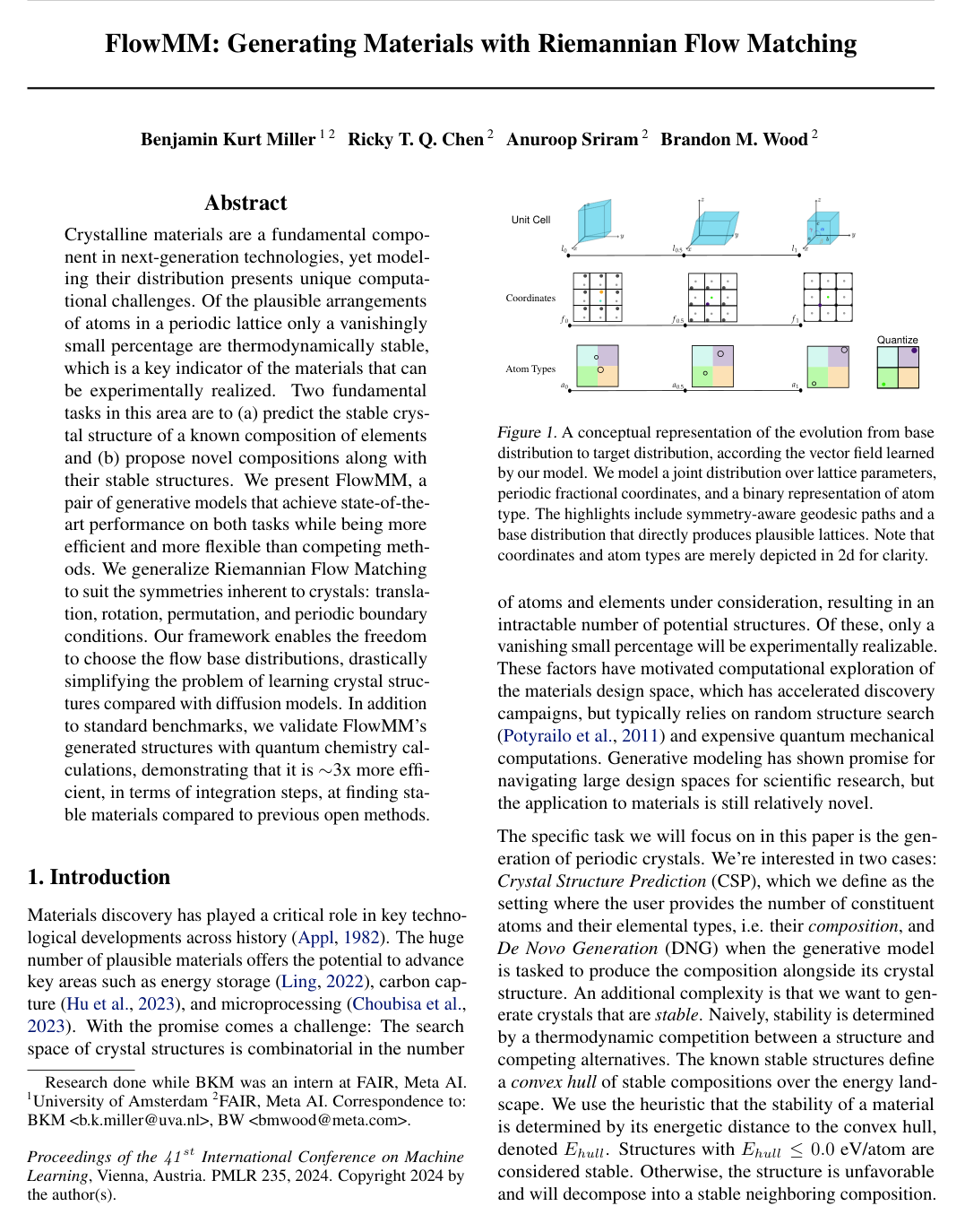
Crystalline materials are a fundamental component in next-generation technologies, yet modeling their distribution presents unique computational challenges. Of the plausible arrangements of atoms in a periodic lattice only a vanishingly small percentage are thermodynamically stable, which is a key indicator of the materials that can be experimentally realized. Two fundamental tasks in this area are to (a) predict the stable crystal structure of a known composition of elements and (b) propose novel compositions along with their stable structures. We present FlowMM, a pair of generative models that achieve state-of-the-art performance on both tasks while being more efficient and more flexible than competing methods. We generalize Riemannian Flow Matching to suit the symmetries inherent to crystals: translation, rotation, permutation, and periodic boundary conditions. Our framework enables the freedom to choose the flow base distributions, drastically simplifying the problem of learning crystal structures compared with diffusion models. In addition to standard benchmarks, we validate FlowMM’s generated structures with quantum chemistry calculations, demonstrating that it is ~3x more efficient, in terms of integration steps, at finding stable materials compared to previous open methods.

Topics

database systems diffusion probabilistic models generative model matching algorithm matching methods distribution functions

Keywords

Riemannian flow matching materials generation crystal structures Matbench Discovery Materials Project database Riemannian manifolds equivariant diffusion structure prediction lattice parameters

1. Introduction
2. Preliminaries
2.1. Representing crystals and their symmetries
2.2. Learning distributions with Flow Matching
2.3. Crystalline Solids
2.4. Problem statements & Datasets
3. Riemannian Flow Matching for Materials
4. Experiments
4.1. Crystal Structure Prediction
4.2. De novo generation
5. Conclusion
Impact Statement
Acknowledgements
References
A. Preliminaries Continued
A.1. Datasets
A.2. Proxy metrics
A.3. Riemannian Manifolds
A.4. Specifics for De Novo Generation
A.5. Symmetry
A.6. Riemannian Flow Matching visualization
A.7. Details about Density Functional Theory calculations
A.8. Limitations of quantifying a computational approach to materials discovery
B. Further Results
B.1. Crystal Structure Prediction (CSP)
B.2. De Novo Generation (DNG)
C. Neural network
D. Enforcing G-invariance of marginal probability path

Knowls

Knowl 1 — Marginal Invariance via Equivalence-Class Riemannian Flow Matching
theoretical result
In generative modeling on Riemannian manifolds subject to symmetry group $G$ (such as spatial rotations $SO(3)$ , permutations $S_n$ , and periodic translations $\tau$ ), a marginal probability path $p_t(x) = \int_{\mathcal{C}} p_t(x \mid x_1) q(x_1) \, dx_1$ connecting a base distribution $p_0 = p$ to a $G$ -invariant target distribution $p_1 = q$ satisfies $G$ -invariance ( $p_t(g \cdot x) = p_t(x)$ for all $g \in G$ ) under either of the following two theorems:

Theorem 1 (Pairwise Invariance): If the conditional probability path $p_t(x \mid x_1)$ is pairwise $G$ -invariant, meaning $p_t(g \cdot x \mid g \cdot x_1) = p_t(x \mid x_1)$ for all $g \in G$ and $x, x_1 \in \mathcal{C}$ , and target distribution $q$ is $G$ -invariant, then the marginal distribution $p_t(x)$ is $G$ -invariant for all $t \in [0, 1]$ .

Theorem 2 (Equivalence-Class Flow Matching): Let $[x_1] = \{g \cdot x_1 \mid g \in G\}$ denote the $G$ -orbit (equivalence class) of $x_1$ . If a $G$ -invariant conditional flow $\psi_t(x_0 \mid x_1)$ satisfies $\psi_t(x_0 \mid g \cdot x_1) = \psi_t(x_0 \mid x_1)$ for all $g \in G$ , and at $t = 1$ concentrates on the equivalence class such that $\psi_1(x_0 \mid x_1) \in [x_1]$ for all $x_0, x_1 \in \mathcal{C}$ , then constructing the unconditional vector field as

$u_t(x) = \int_{\mathcal{C}} u_t(x \mid x_1) \frac{p_t(x \mid x_1) q(x_1)}{p_t(x)} \, dx_1$

generates a marginal probability path $p_t(x) = \int_{\mathcal{C}} p_t(x \mid x_1) q(x_1) \, dx_1$ that satisfies $p_1 = q$ .

This relaxes the standard requirement in flow matching that $p_1(x \mid x_1) = \delta(x - x_1)$ by allowing the conditional path to target the equivalence class $[x_1]$ , which permits the use of entry-wise $G$ -invariant conditional vector fields $u_t(g \cdot x \mid x_1) = u_t(x \mid g \cdot x_1) = u_t(x \mid x_1)$ .
Knowl 2 — Mean-Free Torus Conditional Vector Field and FlowMM Training Objective
equation
For a crystal structure with $n$ atoms represented by atomic types $a \in \mathcal{A}$ , fractional coordinates $f \in [0, 1)^{3 \times n}$ on an $n \times 3$ -dimensional flat torus $\mathbb{T}^{3n}$ , and Niggli-reduced lattice parameters $l \in \mathcal{L} = \mathbb{R}_+^3 \times [60^\circ, 120^\circ]^3$ , the geodesic logarithmic map on the flat torus for atom $i$ is defined by:

$\log_{f_0^i}(f_1^i) = \frac{1}{2\pi} \operatorname{atan2}\left(\sin(\omega^i), \cos(\omega^i)\right), \quad \omega^i = 2\pi(f_1^i - f_0^i)$

To ensure translation invariance under periodic boundary conditions, the conditional vector field on the torus $\mathcal{F}$ subtracts the mean displacement in the tangent space:

$u_t^F(f \mid f_1) = \log_{f_1}(f) - \frac{1}{n} \sum_{i=1}^n \log_{f_1^i}(f^i)$

Given a time $t \sim \operatorname{Uniform}(0, 1)$ , target crystal $c_1 = (a_1, f_1, l_1) \sim q$ , base sample $c_0 = (a_0, f_0, l_0) \sim p$ , and point $c_t$ on the geodesic connecting $c_0$ and $c_1$ at time $t$ , the neural vector field $v_t^\theta(c) = (v_t^{A, \theta}(c), v_t^{F, \theta}(c), v_t^{L, \theta}(c))$ is trained via the dimension-normalized Riemannian Flow Matching objective:

$\mathcal{L}(\theta) = \mathbb{E}_{t, q(c_1), p(c_0)} \left[ \frac{\lambda_a}{hn} \|v_t^{A, \theta}(c_t) + a_0 - a_1\|^2 + \frac{\lambda_f}{3n} \left\|v_t^{F, \theta}(c_t) + \log_{f_1}(f_0) - \frac{1}{n}\sum_{i=1}^n \log_{f_1^i}(f_0^i)\right\|^2 + \frac{\lambda_l}{6} \|v_t^{L, \theta}(c_t) + l_0 - l_1\|^2 \right]$

where $h$ is the categorical dimension of atom types, $\lambda_a, \lambda_f, \lambda_l \in \mathbb{R}_+$ are weighting hyperparameters satisfying $\lambda_a + \lambda_f + \lambda_l = 1$ , and $l$ is mapped to an unconstrained space prior to computing Euclidean flow matching errors.
Knowl 3 — Symmetry-Aware Crystal Representation in FlowMM
model/method
FlowMM represents a periodic crystal containing $n$ atoms as a point $c = (a, f, l) \in \mathcal{C} = \mathcal{A} \times \mathcal{F} \times \mathcal{L}$ on a product Riemannian manifold:
1. Atomic Types ( $a \in \mathcal{A}$ ): For crystal structure prediction (CSP), $a$ is fixed as conditional input. For de novo generation (DNG), $a$ is represented in a continuous analog-bit format in $\mathbb{R}^{\lceil \log_2 h \rceil}$ per atom, where $h$ is the maximum number of chemical element classes, discretized at inference by the sign function $\operatorname{sgn}: \mathbb{R} \to \{-1, 1\}$ .
2. Fractional Coordinates ( $f \in \mathcal{F}$ ): Represented as $f = [f^1, \dots, f^n] \in [0, 1)^{3 \times n}$ on an $n \times 3$ -dimensional flat torus. Physical Cartesian coordinates are $x = \tilde{l} f$ , where $\tilde{l} \in \mathbb{R}^{3 \times 3}$ is the lattice matrix.
3. Lattice Parameters ( $l \in \mathcal{L}$ ): A rotation-invariant representation $l = (a, b, c, \alpha, \beta, \gamma)$ consisting of three side lengths $a, b, c \in \mathbb{R}_+$ (in \AA) and three internal angles $\alpha, \beta, \gamma \in [60^\circ, 120^\circ]$ obtained by Niggli reduction.
This parameterization enforces $SO(3)$ rotational invariance by construction ( $p(Q \cdot c) = p(c)$ for any $Q \in SO(3)$ ), while permutation invariance ( $S_n$ ) and fractional periodic translation invariance ( $\tau \in [-1/2, 1/2]^3$ ) are handled via equivariant graph neural network parameterizations and tangent-space mean subtraction.
Knowl 4 — Base Distributions and Coordinate Diffeomorphisms for Crystal Manifolds
model/method
The base distribution $p(c) = p(a)p(f)p(l)$ over the crystal manifold $\mathcal{C} = \mathcal{A} \times \mathcal{F} \times \mathcal{L}$ in FlowMM is constructed from factorized components that respect domain geometries:
1. Atomic Type Base Distribution: For de novo generation on $\lceil \log_2 h \rceil$ continuous bits per atom, $p(a) = \mathcal{N}(a; 0, I)$ .
2. Fractional Coordinates Base Distribution: Uniform density over the $3n$ -dimensional torus, $p(f) = \operatorname{Uniform}(0, 1)^{3n}$ , ensuring translation invariance $p(\tau \cdot f) = p(f)$ for all periodic translations $\tau \in [-1/2, 1/2]^3$ .
3. Lattice Lengths Base Distribution: For side lengths $(a, b, c) \in \mathbb{R}_+^3$ , an informative prior $p(a, b, c) = \prod_{\eta \in \{a, b, c\}} \operatorname{LogNormal}(\eta; \operatorname{loc}_\eta, \operatorname{scale}_\eta)$ , where parameters $\operatorname{loc}_\eta, \operatorname{scale}_\eta$ are fit to training data via maximum likelihood.
4. Lattice Angles Transformation and Base Distribution: To resolve non-smooth vector fields on the compact boundary $[60^\circ, 120^\circ]^3$ , internal angles $\alpha, \beta, \gamma$ are mapped to unconstrained space $\mathbb{R}^3$ via the diffeomorphism
$\phi(\eta) = \operatorname{logit}\left(\frac{\eta - 60}{120}\right) = \log\left(\frac{\eta - 60}{180 - \eta}\right), \quad \phi^{-1}(\eta') = 120 \, \frac{\exp(\eta')}{1 + \exp(\eta')} + 60$

In the constrained space, the prior is $p(\alpha, \beta, \gamma) = \operatorname{Uniform}(60, 120)^3$ . Flow matching and numerical ODE integration occur in the unconstrained coordinate space $\mathbb{R}^3$ , with samples mapped back to $[60^\circ, 120^\circ]$ via $\phi^{-1}$ .
Knowl 5 — Analog Bit Representation and Sigmoid Cross-Entropy Loss for Element Types
model/method
In de novo material generation (DNG), discrete element types are mapped from categorical one-hot vectors of dimension $h$ to continuous binary analog bits of dimension $\lceil \log_2 h \rceil$ (requiring 7 dimensions per atom for $h = 100$ elements, compared to 100 for one-hot representations).

During training, continuous Normal noise $a_0 \sim \mathcal{N}(0, I)$ flows toward target bit vectors $a_1 \in \{-1, 1\}^{\lceil \log_2 h \rceil}$ . In addition to the velocity matching loss, training incorporates an auxiliary sigmoid cross-entropy loss:

$\mathcal{L}_{\text{sce}} = -\log \sigma(a_1 \cdot \hat{a}_1), \quad \hat{a}_1 := (1 - t) \dot{a}_t + a_t$

where $\sigma(z) = (1 + e^{-z})^{-1}$ is the logistic sigmoid, $a_t = (1 - t)a_0 + t a_1$ , $\dot{a}_t = v_t^{A, \theta}(c_t)$ is the predicted velocity, and $\hat{a}_1$ is the first-order Taylor estimate of the state at $t = 1$ . The total loss includes $\mathcal{L}_{\text{sce}}$ weighted by Lagrange multiplier $\lambda_{\text{sce}}$ . At inference time, discrete atom types are recovered using the sign function $\operatorname{sgn}(a) \in \{-1, 1\}$ .
Knowl 6 — Inference Anti-Annealing Velocity Scheduling
model/method
During inference sampling, the generation ordinary differential equation (ODE) governing the state path $\psi_t^\theta(c)$ from $t = 0$ to $t = 1$ is modified by a time-dependent velocity scaling factor $s(t)$ :

$\frac{d}{dt} \psi_t^\theta(c) = s(t) v_t^\theta(\psi_t^\theta(c)), \quad \psi_0^\theta(c) = c \sim p(c)$

where $s(t) := 1 + s' t$ and $s' \ge 0$ is a scalar hyperparameter (typically $0 \le s' \le 10$ ).

In Crystal Structure Prediction (CSP), anti-annealing is selectively applied only to fractional coordinates $f$ while keeping the lattice velocity unscaled ( $s(t) = 1$ for $l$ ), which significantly increases reconstruction match rate while avoiding distortion of the unit cell. In De Novo Generation (DNG), velocity anti-annealing is applied to both fractional coordinates $f$ and lattice parameters $l$ .
Knowl 7 — Material Stability and S.U.N. Metric Evaluation Framework
definition
For de novo crystal generation, thermodynamic stability and generation efficiency on a generation budget of $N_{\text{gen}}$ samples are quantified by:
1. Stability Rate: Proportion of generated crystals with energy above the Materials Project convex hull $E_{\text{hull}} \le 0.0\text{ eV/atom}$ (determined via density functional theory relaxation with CHGNet prerelaxation) and arity $N\text{-ary} \ge 2$ (excluding unphysical 1-ary false positives):
$\text{Stability Rate} = \frac{N_{\text{stable}}}{N_{\text{gen}}}$
1. S.U.N. Rate: Proportion of generated crystals that are Stable ( $E_{\text{hull}} \le 0.0\text{ eV/atom}$ ), Unique (no duplicates within generated set using pymatgen StructureMatcher), and Novel (no matches among training set crystals sharing the same element set):
$\text{S.U.N. Rate} = \frac{N_{\text{S.U.N.}}}{N_{\text{gen}}}$
1. Inference Compute Costs: Average number of numerical ODE/diffusion integration steps $N_{\text{int. steps}}$ required to find a stable or S.U.N. material:
$\text{Cost} = \frac{N_{\text{int. steps}}}{\text{Stability Rate}}, \quad \text{S.U.N. Cost} = \frac{N_{\text{int. steps}}}{\text{S.U.N. Rate}}$

Knowl 8 — Empirical Performance on Crystal Structure Prediction Benchmarks

data/table

Crystal structure prediction (CSP) performance was evaluated on Perov-5, Carbon-24, MP-20 (up to 20 atoms/cell), and MPTS-52 (chronological split, up to 52 atoms/cell) using StructureMatcher tolerances (stol = 0.5, angle_tol = 10, ltol = 0.3). DiffCSP and FlowMM share identical graph neural network backbones.

Method	Perov-5		Carbon-24		MP-20		MPTS-52
	Match Rate (%) $\uparrow$	RMSE $\downarrow$	Match Rate (%) $\uparrow$	RMSE $\downarrow$	Match Rate (%) $\uparrow$	RMSE $\downarrow$	Match Rate (%) $\uparrow$	RMSE $\downarrow$
CDVAE	45.31	0.1138	17.09	0.2969	33.90	0.1045	5.34	0.2106
DiffCSP	52.02	0.0760	17.54	0.2759	51.49	0.0631	12.19	0.1786
FlowMM	53.15	0.0992	23.47	0.4122	61.39	0.0566	17.54	0.1726

FlowMM outperforms DiffCSP by 9.90 percentage points in Match Rate on MP-20 and 5.35 percentage points on MPTS-52. Furthermore, FlowMM achieves its maximum match rate on MP-20 within approximately 50 ODE integration steps, compared to the 1000 diffusion steps required by DiffCSP.

Knowl 9 — Empirical Performance on De Novo Generation and Sampling Efficiency

data/table

De novo generation (DNG) was evaluated on MP-20 over 10,000 generated structures per run, comparing CDVAE, DiffCSP (1000 steps), and FlowMM across 250, 500, 750, and 1000 ODE integration steps. Density functional theory (DFT) relaxations were performed to compute true $E_{\text{hull}}$ stability.

Method	Steps	Validity (%) $\uparrow$		Coverage (%) $\uparrow$		Property W-Dist $\downarrow$		Stability $\uparrow$	Cost $\downarrow$	S.U.N. Rate $\uparrow$	S.U.N. Cost $\downarrow$
		Struct.	Comp.	Recall	Prec.	$w_{\text{dist}}(\rho)$	$w_{\text{dist}}(N_{\text{el}})$	Rate (%)	Steps/Stab.	Rate (%)	Steps/S.U.N.
CDVAE	5000	100.00	86.70	99.15	99.49	0.688	0.278	1.57	31.85	1.43	34.97
DiffCSP	1000	100.00	83.25	99.71	99.76	0.350	0.125	5.06	1.98	3.34	2.99
FlowMM	250	96.58	83.47	99.48	99.65	0.261	0.107	4.32	0.58	2.38	1.05
FlowMM	500	96.86	83.24	99.38	99.63	0.075	0.079	4.19	1.19	2.45	2.04
FlowMM	750	96.78	83.08	99.64	99.63	0.281	0.097	4.14	1.81	2.22	3.38
FlowMM	1000	96.85	83.19	99.49	99.58	0.239	0.083	4.65	2.15	2.34	4.27

FlowMM exhibits superior fidelity to the true chemical element arity distribution ( $w_{\text{dist}}(N_{\text{el}})$ of 0.083--0.107 vs. 0.125 for DiffCSP and 0.278 for CDVAE) and density ( $w_{\text{dist}}(\rho)$ ). Operating at 250 integration steps, FlowMM achieves an S.U.N. Cost of 1.05 steps per stable, unique, and novel material, representing an approximate $3\times$ efficiency gain over DiffCSP (2.99 steps/S.U.N.).

Knowl 10 — Limitations of Generative Crystal Modeling and DFT Stability Assessment
limitation
The methodology and evaluation framework are subject to four key limitations:
1. Physical Assumptions of DFT: Energy and convex hull stability calculations assume an unphysical ground state at $T = 0\text{ K}$ and $P = 0\text{ atm}$ , ignoring temperature, pressure, entropic contributions, defects, and non-homogeneous crystal disorder.
2. Equivalence and Structure Matching Artifacts: The pymatgen StructureMatcher heuristic relies on fixed distance/angle tolerance thresholds and is not strictly an equivalence relation due to non-transitivity/reflexivity edge cases, potentially misclassifying novel structures or grouping distinct chemical phases.
3. Distributional Interpolation vs. Out-of-Distribution Discovery: Continuous normalizing flows optimize probability density over known empirical training distributions, generating materials primarily through interpolation between known phases rather than discovering radically distinct, out-of-distribution crystal structures.
4. Inference Compute Scope: Generation cost metrics account solely for numerical integration steps during sampling; they omit the computational overhead of model training, surrogate prerelaxation (CHGNet), and final DFT relaxation.

Coverage note — Specific GNN message passing architectural layers (adapted directly from EGNN and DiffCSP) and minor validation sweep hyperparameter tables were omitted in favor of the primary generative modeling contributions, theoretical results, and empirical evaluation data.

References

1.Adams, R. P. and Orbanz, P. Representing and learning functions invariant under crystallographic groups. arXiv preprint arXiv:2306.05261, 2023.
2.AI4Science, M., Hernandez-Garcia, A., Duval, A., Volokhova, A., Bengio, Y., Sharma, D., Carrier, P. L., Koziarski, M., and Schmidt, V. Crystal-gfn: sampling crystals with desirable properties and constraints. arXiv preprint arXiv:2310.04925, 2023.
3.Appl, M. The haber–bosch process and the development of chemical engineering. a century of chemical engineering, 1982.
4.Austin, J., Johnson, D. D., Ho, J., Tarlow, D., and Van Den Berg, R. Structured denoising diffusion models in discrete state-spaces. Advances in Neural Information Processing Systems, 34:17981–17993, 2021.
5.Baird, S. G., Sayeed, H. M., and Riebesell, J. sparks-baird/matbench-genmetrics. https://github.com/sparks-baird/matbench-genmetrics, 2024. [Accessed 03-05-2024].
6.Bose, A. J., Akhound-Sadegh, T., Fatras, K., Huguet, G., Rector-Brooks, J., Liu, C.-H., Nica, A. C., Korablyov, M., Bronstein, M., and Tong, A. Se (3)-stochastic flow matching for protein backbone generation. arXiv preprint arXiv:2310.02391, 2023.
7.Cao, Z., Luo, X., Lv, J., and Wang, L. Space group informed transformer for crystalline materials generation, 2024.
8.Castelli, I. E., Landis, D. D., Thygesen, K. S., Dahl, S., Chorkendorff, I., Jaramillo, T. F., and Jacobsen, K. W. New cubic perovskites for one-and two-photon water splitting using the computational materials repository. Energy & Environmental Science, 5(10):9034–9043, 2012.
9.Chavel, I., Randol, B., and Dodziuk, J. (eds.). Eigenvalues in Riemannian Geometry, volume 115 of Pure and Applied Mathematics. Elsevier, 1984. doi: https://doi.org/10.1016/S0079-8169(08)60810-7. URL https://www.sciencedirect.com/science/article/pii/S0079816908608107.
10.Cheetham, A. K. and Seshadri, R. Artificial intelligence driving materials discovery? perspective on the article: Scaling deep learning for materials discovery. Chemistry of Materials, 2024.
11.Chen, R. T. and Lipman, Y. Riemannian flow matching on general geometries. In The Twelfth International Conference on Learning Representations, 2024. URL https://openreview.net/forum?id=g7ohDlTITL.
12.Chen, R. T., Rubanova, Y., Bettencourt, J., and Duvenaud, D. K. Neural ordinary differential equations. Advances in neural information processing systems, 31, 2018.
13.Chen, T., Zhang, R., and Hinton, G. Analog bits: Generating discrete data using diffusion models with self-conditioning. In The Eleventh International Conference on Learning Representations, 2022.
14.Choubisa, H., Todorović, P., Pina, J. M., Parmar, D. H., Li, Z., Voznyy, O., Tamblyn, I., and Sargent, E. H. Interpretable discovery of semiconductors with machine learning. npj Computational Materials, 9(1):117, 2023.
15.Court, C. J., Yildirim, B., Jain, A., and Cole, J. M. 3-d inorganic crystal structure generation and property prediction via representation learning. Journal of chemical information and modeling, 60(10):4518–4535, 2020.
16.Davies, D. W., Butler, K. T., Jackson, A. J., Skelton, J. M., Morita, K., and Walsh, A. Smact: Semiconducting materials by analogy and chemical theory. Journal of Open Source Software, 4(38):1361, 2019.
17.Deng, B., Zhong, P., Jun, K., Riebesell, J., Han, K., Bartel, C. J., and Ceder, G. Chgnet as a pretrained universal neural network potential for charge-informed atomistic modelling. Nature Machine Intelligence, 5(9):1031–1041, 2023.
18.Falorsi, L. and Forre, P. Neural ordinary differential equations on manifolds. arXiv preprint arXiv:2006.06663, 2020.
19.Flam-Shepherd, D. and Aspuru-Guzik, A. Language models can generate molecules, materials, and protein binding sites directly in three dimensions as xyz, cif, and pdb files. arXiv preprint arXiv:2305.05708, 2023.
20.Geiger, M. and Smidt, T. e3nn: Euclidean neural networks. arXiv preprint arXiv:2207.09453, 2022.
21.Gemici, M. C., Rezende, D., and Mohamed, S. Normalizing flows on riemannian manifolds. arXiv preprint arXiv:1611.02304, 2016.
22.Glass, C. W., Oganov, A. R., and Hansen, N. Uspex—evolutionary crystal structure prediction. Computer physics communications, 175(11-12):713–720, 2006.
23.Grosse-Kunstleve, R. W., Sauter, N. K., and Adams, P. D. Numerically stable algorithms for the computation of reduced unit cells. Acta Crystallographica Section A: Foundations of Crystallography, 60(1):1–6, 2004.
24.Gruver, N., Sriram, A., Madotto, A., Wilson, A. G., Zitnick, C. L., and Ulissi, Z. Fine-tuned language models generate stable inorganic materials as text. arXiv preprint arXiv:2402.04379, 2024.
25.Ho, J., Jain, A., and Abbeel, P. Denoising diffusion probabilistic models. Advances in Neural Information Processing Systems, 33:6840–6851, 2020.
26.Hoogeboom, E., Satorras, V. G., Vignac, C., and Welling, M. Equivariant diffusion for molecule generation in 3d. In International Conference on Machine Learning, pp. 8867–8887. PMLR, 2022.
27.Hu, E., Liu, C., Zhang, W., and Yan, Q. Machine learning assisted understanding and discovery of co2 reduction reaction electrocatalyst. The Journal of Physical Chemistry C, 127(2):882–893, 2023.
28.Huang, C.-W., Aghajohari, M., Bose, J., Panangaden, P., and Courville, A. Riemannian diffusion models. In Oh, A. H., Agarwal, A., Belgrave, D., and Cho, K. (eds.), Advances in Neural Information Processing Systems, 2022.
29.Jain, A., Ong, S. P., Hautier, G., Chen, W., Richards, W. D., Dacek, S., Cholia, S., Gunter, D., Skinner, D., Ceder, G., and Persson, K. A. The Materials Project: A materials genome approach to accelerating materials innovation. APL Materials, 1(1):011002, 07 2013. ISSN 2166-532X. doi: 10.1063/1.4812323. URL https://doi.org/10.1063/1.4812323.
30.Jiao, R., Huang, W., Lin, P., Han, J., Chen, P., Lu, Y., and Liu, Y. Crystal structure prediction by joint equivariant diffusion. arXiv preprint arXiv:2309.04475, 2023.
31.Jiao, R., Huang, W., Liu, Y., Zhao, D., and Liu, Y. Space group constrained crystal generation, 2024.
32.Kohler, J., Klein, L., and Noe, F. Equivariant flows: exact likelihood generative learning for symmetric densities. In International conference on machine learning, pp. 5361–5370. PMLR, 2020.
33.Kohn, W. and Sham, L. J. Self-consistent equations including exchange and correlation effects. Physical review, 140(4A):A1133, 1965.
34.Kondor, R. and Trivedi, S. On the generalization of equivariance and convolution in neural networks to the action of compact groups. In International Conference on Machine Learning, pp. 2747–2755. PMLR, 2018.
35.Kresse, G. and Furthmuller, J. Efficient iterative schemes for ab initio total-energy calculations using a plane-wave basis set. Physical review B, 54(16):11169, 1996.
36.Liao, Y.-L., Wood, B., Das, A., and Smidt, T. Equiformerv2: Improved equivariant transformer for scaling to higher-degree representations. arXiv preprint arXiv:2306.12059, 2023.
37.Ling, C. A review of the recent progress in battery informatics. npj Computational Materials, 8(1):33, 2022.
38.Lipman, Y., Chen, R. T., Ben-Hamu, H., Nickel, M., and Le, M. Flow matching for generative modeling. In The Eleventh International Conference on Learning Representations, 2022.
39.Loshchilov, I. and Hutter, F. Decoupled weight decay regularization. In International Conference on Learning Representations, 2018.
40.Mathieu, E. and Nickel, M. Riemannian continuous normalizing flows. Advances in Neural Information Processing Systems, 33:2503–2515, 2020.
41.Merchant, A., Batzner, S., Schoenholz, S. S., Aykol, M., Cheon, G., and Cubuk, E. D. Scaling deep learning for materials discovery. Nature, pp. 1–6, 2023.
42.Miller, B. K., Geiger, M., Smidt, T. E., and Noe, F. Relevance of rotationally equivariant convolutions for predicting molecular properties. arXiv preprint arXiv:2008.08461, 2020.
43.Nouira, A., Sokolovska, N., and Crivello, J.-C. Crystalgan: learning to discover crystallographic structures with generative adversarial networks. arXiv preprint arXiv:1810.11203, 2018.
44.Ong, S. P., Richards, W. D., Jain, A., Hautier, G., Kocher, M., Cholia, S., Gunter, D., Chevrier, V. L., Persson, K. A., and Ceder, G. Python materials genomics (pymatgen): A robust, open-source python library for materials analysis. Computational Materials Science, 68:314–319, 2013.
45.Passaro, S. and Zitnick, C. L. Reducing so (3) convolutions to so (2) for efficient equivariant gnns. arXiv preprint arXiv:2302.03655, 2023.
46.Perdew, J. P., Burke, K., and Ernzerhof, M. Generalized gradient approximation made simple. Physical review letters, 77(18):3865, 1996.
47.Pickard, C. J. Airss data for carbon at 10gpa and the c+n+h+o system at 1gpa. Materials Cloud Archive, 2020.0026/v1, 2020. doi: 10.24435/materialscloud:2020.0026/v1.
48.Pickard, C. J. and Needs, R. Ab initio random structure searching. Journal of Physics: Condensed Matter, 23(5):053201, 2011.
49.Potyrailo, R., Rajan, K., Stoewe, K., Takeuchi, I., Chisholm, B., and Lam, H. Combinatorial and high-throughput screening of materials libraries: review of state of the art. ACS combinatorial science, 13(6):579–633, 2011.
50.Riebesell, J. Matbench Discovery v1.0.0. figshare, 1 2024. doi: 10.6084/m9.figshare.22715158.v12. URL https://figshare.com/articles/dataset/Matbench_Discovery_v1_0_0/22715158.
51.Riebesell, J., Goodall, R., Benner, P., Chiang, Y., Lee, A., Jain, A., and Persson, K. Matbench Discovery, August 2023a. URL https://github.com/janosh/matbench-discovery.
52.Riebesell, J., Goodall, R. E., Jain, A., Benner, P., Persson, K. A., and Lee, A. A. Matbench discovery an evaluation framework for machine learning crystal stability prediction. arXiv preprint arXiv:2308.14920, 2023b.
53.Satorras, V. G., Hoogeboom, E., and Welling, M. E (n) equivariant graph neural networks. In International conference on machine learning, pp. 9323–9332. PMLR, 2021.
54.Schmidt, J., Hoffmann, N., Wang, H.-C., Borlido, P., Carrico, P. J., Cerqueira, T. F., Botti, S., and Marques, M. A. Large-scale machine-learning-assisted exploration of the whole materials space. arXiv preprint arXiv:2210.00579, 2022.
55.Shaul, N., Chen, R. T., Nickel, M., Le, M., and Lipman, Y. On kinetic optimal probability paths for generative models. In International Conference on Machine Learning, pp. 30883–30907. PMLR, 2023.
56.Sohl-Dickstein, J., Weiss, E., Maheswaranathan, N., and Ganguli, S. Deep unsupervised learning using nonequilibrium thermodynamics. In International Conference on Machine Learning, pp. 2256–2265. PMLR, 2015.
57.Song, Y., Sohl-Dickstein, J., Kingma, D. P., Kumar, A., Ermon, S., and Poole, B. Score-based generative modeling through stochastic differential equations. arXiv preprint arXiv:2011.13456, 2020.
58.Thomas, N., Smidt, T., Kearnes, S., Yang, L., Li, L., Kohlhoff, K., and Riley, P. Tensor field networks: Rotation-and translation-equivariant neural networks for 3d point clouds. arXiv preprint arXiv:1802.08219, 2018.
59.Wang, H.-C., Botti, S., and Marques, M. A. Predicting stable crystalline compounds using chemical similarity. npj Computational Materials, 7(1):12, 2021.
60.Ward, L., Agrawal, A., Choudhary, A., and Wolverton, C. A general-purpose machine learning framework for predicting properties of inorganic materials. npj Computational Materials, 2(1):1–7, 2016.
61.Weiler, M., Forre, P., Verlinde, E., and Welling, M. Coordinate independent convolutional networks–isometry and gauge equivariant convolutions on riemannian manifolds. arXiv preprint arXiv:2106.06020, 2021.
62.Wirnsberger, P., Papamakarios, G., Ibarz, B., Racaniere, S., Ballard, A. J., Pritzel, A., and Blundell, C. Normalizing flows for atomic solids. Machine Learning: Science and Technology, 3(2):025009, 2022.
63.Xie, T., Fu, X., Ganea, O.-E., Barzilay, R., and Jaakkola, T. S. Crystal diffusion variational autoencoder for periodic material generation. In International Conference on Learning Representations, 2021.
64.Yang, M., Cho, K., Merchant, A., Abbeel, P., Schuurmans, D., Mordatch, I., and Cubuk, E. D. Scalable diffusion for materials generation. arXiv preprint arXiv:2311.09235, 2023.
65.Yang, W., Siriwardane, E. M. D., Dong, R., Li, Y., and Hu, J. Crystal structure prediction of materials with high symmetry using differential evolution. Journal of Physics: Condensed Matter, 33(45):455902, 2021.
66.Yim, J., Campbell, A., Foong, A. Y., Gastegger, M., Jimenez-Luna, J., Lewis, S., Satorras, V. G., Veeling, B. S., Barzilay, R., Jaakkola, T., et al. Fast protein backbone generation with se (3) flow matching. arXiv preprint arXiv:2310.05297, 2023.
67.Zeni, C., Pinsler, R., Zugner, D., Fowler, A., Horton, M., Fu, X., Shysheya, S., Crabbe, J., Sun, L., Smith, J., et al. Mattergen: a generative model for inorganic materials design. arXiv preprint arXiv:2312.03687, 2023.
68.Zimmermann, N. E. and Jain, A. Local structure order parameters and site fingerprints for quantification of coordination environment and crystal structure similarity. RSC advances, 10(10):6063–6081, 2020.

Citation

MLA

Miller, B. K., et al. “FlowMM: Generating Materials with Riemannian Flow Matching”. ICML 2024, 2024, http://arxiv.org/abs/2406.04713v1.

APA

Miller, B. K., Chen, R. T. Q., Sriram, A., & Wood, B. M. (2024). FlowMM: Generating Materials with Riemannian Flow Matching. ICML 2024. http://arxiv.org/abs/2406.04713v1

Chicago

Miller, B. K., R. T. Q. Chen, A. Sriram, and B. M. Wood. 2024. “FlowMM: Generating Materials with Riemannian Flow Matching”. ICML 2024. http://arxiv.org/abs/2406.04713v1.

Harvard

Miller, B.K. et al. (2024) “FlowMM: Generating Materials with Riemannian Flow Matching”, ICML 2024 [Preprint]. Available at: http://arxiv.org/abs/2406.04713v1.

Vancouver

1. Miller BK, Chen RTQ, Sriram A, Wood BM (2024) FlowMM: Generating Materials with Riemannian Flow Matching. ICML 2024

BibTeX

@article{miller2024flowmm,
  title = {FlowMM: Generating Materials with Riemannian Flow Matching},
  author = {Miller, Benjamin Kurt and Chen, Ricky T. Q. and Sriram, Anuroop and Wood, Brandon M},
  year = {2024},
  journal = {ICML 2024},
  url = {http://arxiv.org/abs/2406.04713v1},
  eprint = {2406.04713}
}

Metadata:arXiv

Source Code

This paper has an official code repository available. Click below to access the source code.

View Repository

Access the Paper

This paper is available from its original source. Click below to access the PDF.

Open PDF

License: https://creativecommons.org/licenses/by/4.0/

FlowMM: Generating Materials with Riemannian Flow Matching

Abstract

Topics

Keywords

Table of Contents

Knowls

Knowl 1 — Marginal Invariance via Equivalence-Class Riemannian Flow Matching

Knowl 2 — Mean-Free Torus Conditional Vector Field and FlowMM Training Objective

Knowl 3 — Symmetry-Aware Crystal Representation in FlowMM

Knowl 4 — Base Distributions and Coordinate Diffeomorphisms for Crystal Manifolds

Knowl 5 — Analog Bit Representation and Sigmoid Cross-Entropy Loss for Element Types

Knowl 6 — Inference Anti-Annealing Velocity Scheduling

Knowl 7 — Material Stability and S.U.N. Metric Evaluation Framework