Generative AI models based on diffusion and flow matching have achieved remarkable quality but traditionally require many iterative steps to produce a single image, making them slow and costly to run. Recent attempts to reduce this to a single step have struggled with poor quality or required complex training procedures like distillation from pre-trained models or curriculum learning. This work addresses whether it is possible to train a high-quality one-step generative model from scratch using a principled mathematical framework.
Approach
The researchers introduced MeanFlow, a new method based on modeling average velocity rather than the instantaneous velocity used in standard Flow Matching. Average velocity is the displacement between two time points divided by the time interval. They derived a mathematical identity—the MeanFlow Identity—that relates average velocity to instantaneous velocity through a time derivative term. This identity does not depend on any specific neural network architecture; it is an intrinsic property of the underlying mathematical field.
The training procedure uses this identity to construct a regression target for a neural network. The target combines the instantaneous velocity (which can be computed directly from training data) with a correction term involving the network's own gradients, computed efficiently using a Jacobian-vector product operation. At inference time, generating an image requires only a single evaluation of the trained network.
The method was tested primarily on ImageNet 256×256 image generation, comparing against previous one-step methods and multi-step baselines. Models were trained entirely from scratch without distillation, pre-training, or curriculum learning. The team also tested scalability by training models of different sizes and for different durations.
Key findings
MeanFlow achieved an FID score of 3.43 on ImageNet 256×256 with just one function evaluation, a 50-70% relative improvement over the previous best one-step methods (which scored between 7.77 and 10.60 FID). With two evaluations, the method achieved 2.20 FID, matching the performance of leading multi-step models that require 500 evaluations (DiT at 2.27 FID and SiT at 2.15 FID).
The model demonstrates strong scalability: larger models and longer training consistently improve quality, following the same scaling behavior seen in standard diffusion models. On CIFAR-10, MeanFlow performed competitively with specialized one-step methods (2.92 FID versus 2.83-3.60 for others).
Ablation studies confirmed that each component matters. The ratio of training samples where the two time variables differ significantly affects quality, with 25% being optimal. The Jacobian-vector product computation, though it adds computational cost, is essential—removing it breaks the method. Different ways of encoding the time variables all work reasonably well, but encoding time and time-interval performs best. The choice of loss metric matters substantially, with adaptively weighted losses outperforming standard squared error.
The method naturally supports classifier-free guidance during training, allowing guidance to improve quality at inference time without requiring additional network evaluations.
What this means
This work largely closes the gap between one-step and multi-step generative models in terms of quality. Previously, achieving high quality required either many sampling steps or complex distillation procedures from pre-trained models. MeanFlow shows that with the right mathematical framework, one-step generation can be trained directly and achieve results competitive with methods requiring hundreds of steps.
This has direct implications for deployment cost and latency. A model requiring one evaluation instead of 250 can generate images 250 times faster and at a fraction of the computational cost. This makes high-quality generative AI more practical for real-time applications, edge deployment, and scenarios where inference cost is a major constraint.
The result also challenges the prevailing assumption that one-step generation is fundamentally limited compared to iterative methods. The quality gap was not due to an inherent mathematical limitation but rather to the lack of a proper training framework.
Recommendations and next steps
Organizations deploying generative models should evaluate MeanFlow-based architectures for applications where inference cost or latency is a concern. The method is production-ready, having been trained and validated at scale on standard benchmarks.
For research teams, the main opportunity is to combine MeanFlow with orthogonal improvements such as better network architectures or advanced training techniques, which were not explored in this work. The mathematical framework is general and should transfer to other domains beyond image generation, such as video, audio, or 3D content.
Before deploying in production, teams should validate performance on their specific data distributions and quality metrics, as the current results are based on academic benchmarks. For applications requiring extremely high fidelity or specific visual characteristics, testing whether one-step generation meets requirements is essential.
Further work is needed to understand the theoretical limits of one-step generation—whether there are fundamental quality ceilings or whether continued scaling can match or exceed current multi-step methods in all scenarios.
Limitations and confidence
The method was validated primarily on ImageNet at 256×256 resolution and CIFAR-10 at 32×32 resolution. Performance on other data types, higher resolutions, or different modalities (video, 3D, etc.) remains to be demonstrated.
The training still requires substantial computational resources—models were trained for up to 1000 epochs on large datasets using specialized hardware (TPUs). While inference is dramatically cheaper than multi-step methods, training cost remains high.
The Jacobian-vector product computation adds about 20% overhead to training time compared to standard Flow Matching. While acceptable for the quality gains achieved, this is a concrete cost that cannot be eliminated.
The results are strong and the mathematical derivation is sound, giving high confidence in the core findings. The method's performance advantage over previous one-step approaches is large and consistent across model sizes and training durations, suggesting the results are robust rather than artifacts of a specific setup.
In this section, the authors introduce MeanFlow, a principled framework for one-step generative modeling that addresses the limitations of existing flow-based methods. Rather than modeling instantaneous velocity as in Flow Matching, MeanFlow characterizes flow fields using average velocity—the ratio of displacement to time interval. A rigorous identity connecting average and instantaneous velocities emerges from this definition and guides neural network training without requiring pre-training, distillation, or curriculum learning. The method is self-contained and theoretically grounded, ensuring that the optimal solution depends on the underlying field rather than network-specific heuristics. On ImageNet 256×256, MeanFlow achieves an FID of 3.43 with just one function evaluation when trained from scratch, outperforming previous state-of-the-art one-step diffusion and flow models by 50-70%. This work substantially closes the performance gap between one-step and multi-step generative models, offering a foundation for rethinking diffusion and flow-based frameworks.
We propose a principled and effective framework for one-step generative modeling. We introduce the notion of average velocity to characterize flow fields, in contrast to instantaneous velocity modeled by Flow Matching methods. A well-defined identity between average and instantaneous velocities is derived and used to guide neural network training. Our method, termed the MeanFlow model, is self-contained and requires no pre-training, distillation, or curriculum learning. MeanFlow demonstrates strong empirical performance: it achieves an FID of 3.43 with a single function evaluation (1-NFE) on ImageNet 256 ×\times× 256 trained from scratch, significantly outperforming previous state-of-the-art one-step diffusion/flow models. Our study substantially narrows the gap between one-step diffusion/flow models and their multi-step predecessors, and we hope it will motivate future research to revisit the foundations of these powerful models.
Figure 1:One-step generation on ImageNet 256 × 256 from scratch. Our MeanFlow (MF) model achieves significantly better generation quality than previous state-of-the-art one-step diffusion/flow methods. Here, iCT [1], Shortcut [2], and our MF are all 1-NFE generation, while IMM's 1-step result [3] involves 2-NFE guidance. Detailed numbers are in Tab. 2. Images shown are generated by our 1-NFE model.
💭 Click to ask about this figure
1 Introduction
Show me a brief summary.
In this section, the authors introduce MeanFlow, a principled framework for one-step generative modeling that addresses limitations in existing diffusion and flow-based approaches. While Flow Matching and diffusion models typically require iterative sampling and model instantaneous velocities, recent one-step methods like Consistency Models impose behavioral constraints on neural networks without well-defined ground-truth fields, leading to unstable training that requires careful curriculum design. MeanFlow instead models average velocity—the ratio of displacement to time interval—and derives an intrinsic mathematical relation between average and instantaneous velocities that naturally guides training without additional heuristics. This framework trains networks from scratch without pre-training, distillation, or curriculum learning, and can incorporate classifier-free guidance at no sampling-time cost. On ImageNet 256×256, MeanFlow achieves an FID of 3.43 with single function evaluation, outperforming previous state-of-the-art one-step methods by 50-70% and substantially narrowing the gap with multi-step predecessors.
The goal of generative modeling is to transform a prior distribution into the data distribution. Flow Matching [4, 5, 6] provides an intuitive and conceptually simple framework for constructing flow paths that transport one distribution to another. Closely related to diffusion models [7, 8, 9], Flow Matching focuses on the velocity fields that guide model training. Since its introduction, Flow Matching has seen widespread adoption in modern generative modeling [10, 11, 12].
Both Flow Matching and diffusion models perform iterative sampling during generation. Recent research has paid significant attention to few-step—and in particular, one-step, feedforward—generative models. Pioneering this direction, Consistency Models [13, 1, 14, 15] introduce a consistency constraint to network outputs for inputs sampled along the same path. Despite encouraging results, the consistency constraint is imposed as a property of the network's behavior, while the properties of the underlying ground-truth field that should guide learning remain unknown. Consequently, training can be unstable and requires a carefully designed "discretization curriculum" [13, 1, 14] to progressively constrain the time domain.
In this work, we propose a principled and effective framework, termed MeanFlow, for one-step generation. The core idea is to introduce a new ground-truth field representing the average velocity, in contrast to the instantaneous velocity typically modeled in Flow Matching. Average velocity is defined as the ratio of displacement to a time interval, with displacement given by the time integral of the instantaneous velocity. Solely originated from this definition, we derive a well-defined, intrinsic relation between the average and instantaneous velocities, which naturally serves as a principled basis for guiding network training.
Building on this fundamental concept, we train a neural network to directly model the average velocity field. We introduce a loss function that encourages the network to satisfy the intrinsic relation between average and instantaneous velocities. No extra consistency heuristic is needed. The existence of the ground-truth target field ensures that the optimal solution is, in principle, independent of the specific network, which in practice can lead to more robust and stable training. We further show that our framework can naturally incorporate classifier-free guidance (CFG) [16] into the target field, incurring no additional cost at sampling time when guidance is used.
Our MeanFlow Models demonstrate strong empirical performance in one-step generative modeling. On ImageNet 256 ×\times× 256 [17], our method achieves an FID of 3.43 using 1-NFE (Number of Function Evaluations) generation. This result significantly outperforms previous state-of-the-art methods in its class by a relative margin of 50% to 70% (Figure 1). In addition, our method stands as a self-contained generative model: it is trained entirely from scratch, without any pre-training, distillation, or curriculum learning. Our study largely closes the gap between one-step diffusion/flow models and their multi-step predecessors, and we hope it will inspire future work to reconsider the foundations of these powerful models.
2 Related Work
Show me a brief summary.
In this section, the authors situate their MeanFlow approach within the broader landscape of diffusion models and Flow Matching methods, which have evolved as powerful generative modeling frameworks that progressively transform noise into data by solving differential equations. While these models traditionally require many iterative sampling steps, recent research has focused on reducing this computational burden through distillation-based approaches that compress pre-trained multi-step models into few-step variants, as well as through standalone methods like Consistency Models that enforce output consistency across different time steps along trajectories. The most relevant recent work explores modeling quantities dependent on two time variables rather than one: Flow Maps capture displacement between time steps, Shortcut Models add self-consistency losses for different time intervals, and Inductive Moment Matching ensures consistency of stochastic interpolants. However, these methods typically impose consistency constraints as heuristic properties of network behavior rather than deriving them from fundamental principles about the underlying velocity fields themselves.
Diffusion and Flow Matching.
Over the past decade, diffusion models [7, 8, 9, 18] have been developed into a highly successful framework for generative modeling. These models progressively add noise to clean data and train a neural network to reverse this process. This procedure involves solving stochastic differential equations (SDE), which is then reformulated as probability flow ordinary differential equations (ODE) [18, 19]. Flow Matching methods [4, 5, 6] extend this framework by modeling the velocity fields that define flow paths between distributions. Flow Matching can also be viewed as a form of continuous-time Normalizing Flows [20].
Few-step Diffusion/Flow Models.
Reducing sampling steps has become an important consideration from both practical and theoretical perspectives. One approach is to distill a pre-trained many-step diffusion model into a few-step model, e.g., [21, 22, 23] or score distillation [24, 25, 26]. Early explorations into training few-step models [13] are built upon the evolution of distillation-based methods. Meanwhile, Consistency Models [13] are developed as a standalone generative model that does not require distillation. These models impose consistency constraints on network outputs at different time steps, encouraging them to produce the same endpoints along the trajectory. Various consistency models and training strategies [13, 1, 14, 15, 27] have been investigated.
In recent work, several methods have focused on characterizing diffusion-/flow-based quantities with respect to two time-dependent variables. In [28], a Flow Map is defined as the integral of the flow between two time steps, with several forms of matching losses developed for learning. In comparison to the average velocity our method is based on, the Flow Map corresponds to displacement. Shortcut Models [2] introduce a self-consistency loss function in addition to Flow Matching, which captures relationships between the flows at different discrete time intervals. Inductive Moment Matching [3] models the self-consistency of stochastic interpolants at different time steps.
3 Background: Flow Matching
Show me a brief summary.
In this section, Flow Matching is presented as a generative modeling framework that learns velocity fields to transport a prior distribution to a data distribution by constructing flow paths between them. The method defines conditional velocities for individual data-noise pairs along these paths, but because a given point can arise from multiple such pairs, Flow Matching actually models the marginal velocity—the expectation over all possible conditional velocities. A neural network is trained to approximate this marginal velocity field by minimizing a conditional Flow Matching loss, which is equivalent to minimizing the intractable marginal loss. During sampling, the learned velocity field guides an ODE solver that integrates the velocity over time to generate samples, though this requires numerical approximation over discrete steps. Critically, even when conditional flows are designed to be straight, the marginal velocity field induces curved trajectories, making coarse discretizations with numerical solvers inaccurate and motivating the need for better one-step generation methods.
Figure 2:Velocity fields in Flow Matching [4]. Left: conditional flows [4]. A given zt can arise from different (x,ϵ) pairs, resulting in different conditional velocities vt. Right: marginal flows [4], obtained by marginalizing over all possible conditional velocities. The marginal velocity field serves as the underlying ground-truth field for network training. All velocities shown here are essentially instantaneous velocities. Illustration follows [29]. (Gray dots: samples from prior; red dots: samples from data.)
💭 Click to ask about this figure
Flow Matching [4, 6, 30] is a family of generative models that learn to match the flows, represented by velocity fields, between two probabilistic distributions. Formally, given data x∼pdata(x)x \sim p_\text{data}(x)x∼pdata(x) and prior ϵ∼pprior(ϵ){\epsilon}\sim p_\text{prior}({\epsilon})ϵ∼pprior(ϵ), a flow path can be constructed as zt=atx+btϵz_t = a_t x + b_t {\epsilon}zt=atx+btϵ with time ttt, where ata_tat and btb_tbt are predefined schedules. The velocity vtv_tvt is defined as vt=zt′=at′x+bt′ϵv_t = z'_t = a'_t x + b'_t {\epsilon}vt=zt′=at′x+bt′ϵ, where ′'′ denotes the time derivative. This velocity is referred to as the conditional velocity in [4], denoted by vt=vt(zt∣x)v_t=v_t(z_t \mid x)vt=vt(zt∣x). See Figure 2 left. A commonly used schedule is at=1−ta_t = 1 - tat=1−t and bt=tb_t = tbt=t, which leads to vt=ϵ−xv_t = {\epsilon} - xvt=ϵ−x.
Because a given ztz_tzt and its vtv_tvt can arise from different xxx and ϵ{\epsilon}ϵ, Flow Matching essentially models the expectation over all possibilities, called the marginal velocity [4] (Figure 2 right):
v(zt,t)≜Ept(vt∣zt)[vt].
💭 Click to ask about this equation
(1)
A neural network vθv_\thetavθ parameterized by θ\thetaθ is learned to fit the marginal velocity field: LFM(θ)=Et,pt(zt)∥vθ(zt,t)−v(zt,t)∥2\mathcal{L}_\text{FM}(\theta) = \mathbb{E}_{t, p_t(z_t)} \| v_\theta(z_t, t) - v(z_t, t) \|^2LFM(θ)=Et,pt(zt)∥vθ(zt,t)−v(zt,t)∥2. Although computing this loss function is infeasible due to the marginalization in Equation 1, it is proposed to instead evaluate the conditional Flow Matching loss [4]: LCFM(θ)=Et,x,ϵ∥vθ(zt,t)−vt(zt∣x)∥2\mathcal{L}_\text{CFM}(\theta) = \mathbb{E}_{t, x, {\epsilon}} \| v_\theta(z_t, t) - v_t(z_t \mid x) \|^2LCFM(θ)=Et,x,ϵ∥vθ(zt,t)−vt(zt∣x)∥2, where the target vtv_tvt is the conditional velocity. Minimizing LCFM\mathcal{L}_\text{CFM}LCFM is equivalent to minimizing LFM\mathcal{L}_\text{FM}LFM [4].
Given a marginal velocity field v(zt,t)v(z_t, t)v(zt,t), samples are generated by solving an ODE for ztz_tzt:
dtdzt=v(zt,t)
💭 Click to ask about this equation
(2)
starting from z1=ϵ∼ppriorz_1= {\epsilon}\sim p_\text{prior}z1=ϵ∼pprior. The solution can be written as: zr=zt−∫rtv(zτ,τ)dτz_r = z_t - \int^t_r v(z_\tau, \tau) d\tauzr=zt−∫rtv(zτ,τ)dτ, where we use rrr to denote another time step. In practice, this integral is approximated numerically over discrete time steps. For example, the Euler method, a first-order ODE solver, computes each step as: zti+1=zti+(ti+1−ti)v(zti,ti)z_{t_{i+1}}=z_{t_i} + (t_{i+1} - t_{i})v(z_{t_i}, t_i)zti+1=zti+(ti+1−ti)v(zti,ti). Higher-order solvers can also be applied.
It is worth noting that even when the conditional flows are designed to be straight ("rectified") [4, 6], the marginal velocity field Equation (1) typically induces a curved trajectory. See Figure 2 for illustration. We also emphasize that this non-straightness is not only a result of neural network approximation, but rather arises from the underlying ground-truth marginal velocity field. When applying coarse discretizations over curved trajectories, numerical ODE solvers lead to inaccurate results.
4 MeanFlow Models
Show me a brief summary.
In this section, the authors introduce MeanFlow, a principled framework for one-step generative modeling that fundamentally differs from Flow Matching by modeling average velocity instead of instantaneous velocity. Average velocity is defined as displacement over a time interval, and by differentiating this definition with respect to time, they derive the MeanFlow Identity—a mathematical relationship showing that average velocity equals instantaneous velocity minus a correction term involving the time derivative of average velocity. This identity enables tractable training by providing an effective regression target that depends only on the accessible instantaneous velocity and efficiently computed Jacobian-vector products, avoiding costly integral computations. The method naturally extends to classifier-free guidance by defining guided velocity fields and their corresponding average velocities, allowing single-step sampling with guidance at no additional inference cost. Through careful design choices in loss metrics, time step sampling distributions, and network conditioning strategies, MeanFlow achieves stable training from scratch without requiring pre-training, distillation, or curriculum learning, demonstrating strong empirical performance in one-step generation tasks.
4.1 Mean Flows
The core idea of our approach is to introduce a new field representing average velocity, whereas the velocity modeled in Flow Matching represents the instantaneous velocity.
Average Velocity.
We define average velocity as the displacement between two time steps ttt and rrr (obtained by integration) divided by the time interval. Formally, the average velocity uuu is:
u(zt,r,t)≜t−r1∫rtv(zτ,τ)dτ.
💭 Click to ask about this equation
(3)
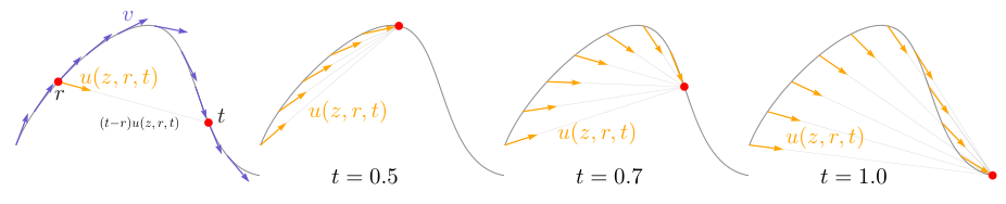
To emphasize the conceptual difference, throughout this paper, we use the notation uuu to denote average velocity, and vvv to denote instantaneous velocity. u(zt,r,t)u(z_t, r, t)u(zt,r,t) is a field that is jointly dependent on (r,t)(r, t)(r,t). The field of uuu is illustrated in Figure 3. Note that in general, the average velocity uuu is the result of a functional of the instantaneous velocity vvv: that is, u=F[v]≜1t−r∫rtvdτu = \mathcal{F}[v] \triangleq \frac{1}{t-r}\int_{r}^{t}vd\tauu=F[v]≜t−r1∫rtvdτ. It is a field induced by vvv, not depending on any neural network. Conceptually, just as the instantaneous velocity vvv serves as the ground-truth field in Flow Matching, the average velocity uuu in our formulation provides an underlying ground-truth field for learning.
Figure 3:The field of average velocityu(z,r,t). Leftmost: While the instantaneous velocityv determines the tangent direction of the path, the average velocity u(z,r,t), defined in Eq. (3), is generally not aligned with v. The average velocity is aligned with the displacement, which is (t−r)u(z,r,t). Right three subplots: The field u(z,r,t) is conditioned on both r and t, and is shown here for t=0.5, 0.7, and 1.0.
💭 Click to ask about this figure
By definition, the field of uuu satisfies certain boundary conditions and
consistency" constraints (generalizing the terminology of [13]). As $r{\rightarrow}t$, we have: $\lim_{r \rightarrow t} u=v$. Moreover, a form of "consistency" is naturally satisfied: taking one larger step over $[r, t]$ is
consistent" with taking two smaller consecutive steps over [r,s][r, s][r,s] and [s,t][s, t][s,t], for any intermediate time sss. To see this, observe that (t−r)u(zt,r,t)=(s−r)u(zs,r,s)+(t−s)u(zt,s,t)(t-r)u(z_t, r, t) = (s-r)u(z_{s}, r, s) + (t-s)u(z_t, s, t)(t−r)u(zt,r,t)=(s−r)u(zs,r,s)+(t−s)u(zt,s,t), which follows directly from the additivity of the integral: ∫rtvdτ=∫rsvdτ+∫stvdτ\int_{r}^{t}vd\tau = \int_{r}^{s}vd\tau + \int_{s}^{t}vd\tau∫rtvdτ=∫rsvdτ+∫stvdτ. Thus, a network that accurately approximates the true uuu is expected to satisfy the consistency relation inherently, without the need for explicit constraints.
The ultimate aim of our MeanFlow model will be to approximate the average velocity using a neural network uθ(zt,r,t)u_\theta(z_t, r, t)uθ(zt,r,t). This has the notable advantage that, assuming we approximate this quantity accurately, we can approximate the entire flow path using a single evaluation of uθ(ϵ,0,1)u_\theta(\epsilon, 0, 1)uθ(ϵ,0,1). In other words, and as we will also demonstrate empirically, the approach is much more amenable to single or few-step generation, as it does not need to explicitly approximate a time integral at inference time, which was required when modeling instantaneous velocity. However, directly using the average velocity defined by Equation 3 as ground truth for training a network is intractable, as it requires evaluating an integral during training. Our key insight is that the definitional equation of average velocity can be manipulated to construct an optimization target that is ultimately amenable to training, even when only the instantaneous velocity is accessible.
The MeanFlow Identity.
To have a formulation amenable to training, we rewrite Equation 3 as:
(t−r)u(zt,r,t)=∫rtv(zτ,τ)dτ.
💭 Click to ask about this equation
(4)
Now we differentiate both sides with respect to ttt, treating rrr as independent of ttt. This leads to:
where the manipulation of the left hand side employs the product rule and the right hand side uses the fundamental theorem of calculus1. Rearranging terms, we obtain the identity:
average vel.u(zt,r,t)ṭd=instant. vel.v(zt,t)ṭd−(t−r)time derivativedtdu(zt,r,t)
💭 Click to ask about this equation
(6)
We refer to this equation as the ``MeanFlow Identity", which describes the relation between vvv and uuu. It is easy to show that Equation 5 and 4 are equivalent (see Appendix B.3).
If r depends on t, the Leibniz rule gives: dtd∫rtv(zτ,τ)dτ=v(zt,t)−v(zr,r)dtdr.
The right hand side of Equation 5 provides a ``target" form for u(zt,r,t)u(z_t, r, t)u(zt,r,t), which we will leverage to construct a loss function to train a neural network. To serve as a suitable target, we must also further decompose the time derivative term, which we discuss next.
Computing Time Derivative.
To compute the ddtu{\frac{d}{d t}}udtdu term in Equation 5, note that ddt{\frac{d}{d t}}dtd denotes a total derivative, which can be expanded in terms of partial derivatives:
dtdu(zt,r,t)=dtdzt∂zu+dtdr∂ru+dtdt∂tu.
💭 Click to ask about this equation
(7)
With dztdt=v(zt,t)\frac{dz_t}{dt}=v(z_t, t)dtdzt=v(zt,t) (see Equation 2), drdt=0\frac{dr}{dt}=0dtdr=0, and dtdt=1\frac{dt}{dt}=1dtdt=1, we have another relation between uuu and vvv:
dtdu(zt,r,t)=v(zt,t)∂zu+∂tu,
💭 Click to ask about this equation
(8)
This equation shows that the total derivative is given by the Jacobian-vector product (JVP) between [∂zu,∂ru,∂tu][\partial_{z}{u}, \partial_{r}{u}, \partial_{t}{u}][∂zu,∂ru,∂tu] (the Jacobian matrix of the function uuu) and the tangent vector [v,0,1][v, 0, 1][v,0,1]. In modern libraries, this can be efficiently computed by the jvp interface, such as torch.func.jvp in PyTorch or jax.jvp in JAX, which we discuss later.
Training with Average Velocity.
Up to this point, the formulations are independent of any network parameterization. We now introduce a model to learn uuu. Formally, we parameterize a network uθu_\thetauθ and encourage it to satisfy the MeanFlow Identity Equation (5). Specifically, we minimize this objective:
The term utgtu_\text{tgt}utgt serves as the effective regression target, which is driven by Equation 5. This target uses the instantaneous velocity vvv as the only ground-truth signal; no integral computation is needed. While the target should involve derivatives of uuu (that is, ∂u\partial u∂u), they are replaced by their parameterized counterparts (that is, ∂uθ\partial u_\theta∂uθ). In the loss function, a stop-gradient (sg) operation is applied on the target utgtu_\text{tgt}utgt, following common practice [13, 1, 14, 15, 2]: in our case, it eliminates the need for “double backpropagation” through the Jacobian-vector product, thereby avoiding higher-order optimization. Despite these practices for optimizability, if uθu_\thetauθ were to achieve zero loss, it is easy to show that it would satisfy the MeanFlow Identity Equation (5), and thus satisfy the original definition Equation (3).
The velocity v(zt,t)v(z_t, t)v(zt,t) in Equation 7b is the marginal velocity in Flow Matching [4] (see Figure 2 right). We follow [4] to replace it with the conditional velocity (Figure 2 left). With this, the target is:
utgt=vt−(t−r)(vt∂zuθ+∂tuθ).
💭 Click to ask about this equation
(11)
Recall that vt=at′x+bt′ϵv_t = a_t'x+b_t'{\epsilon}vt=at′x+bt′ϵ is the conditional velocity [4], and by default, vt=ϵ−xv_t = {\epsilon} - xvt=ϵ−x.
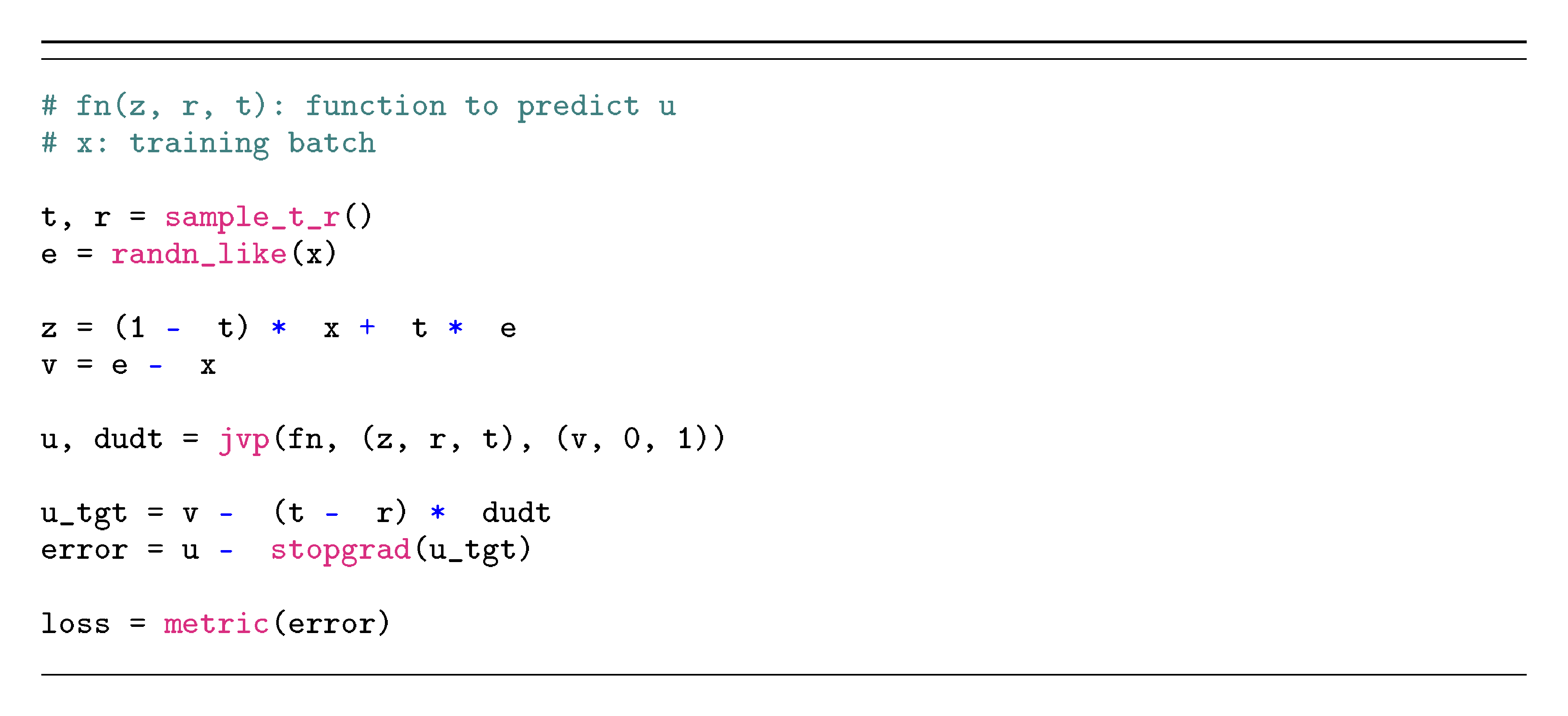
Pseudocode for minimizing the loss function Equation 7a is presented in Algorithm 1. Overall, our method is conceptually simple: it behaves similarly to Flow Matching, with the key difference that the matching target is modified by −(t−r)(vt∂zuθ+∂tuθ)-(t - r) \left (v_t\partial_{z}{u_\theta}+\partial_{t}{u_\theta} \right)−(t−r)(vt∂zuθ+∂tuθ), arising from our consideration of the average velocity. In particular, note that if we were to restrict to the condition t=rt=rt=r, then the second term vanishes, and the method would exactly match standard Flow Matching.
Algorithm 1: MeanFlow: Training. Note: in PyTorch and JAX, jvp returns the function output and JVP.
💭 Click to ask about this figure
Algorithm 2: MeanFlow: 1-step Sampling
e = randn(x_shape)x = e - fn(e, r=0, t=1)
In Algorithm 1, the jvp operation is highly efficient. In essence, computing ddtu{\frac{d}{d t}}udtdu via jvp requires only a single backward pass, similar to standard backpropagation in neural networks. Because ddtu{\frac{d}{d t}}udtdu is part of the target utgtu_\text{tgt}utgt and thus subject to stopgrad (w.r.t.θ\thetaθ), the backpropagation for neural network optimization (w.r.t.θ\thetaθ) treats ddtu{\frac{d}{d t}}udtdu as a constant, incurring no higher-order gradient computation. Consequently, jvp introduces only a single extra backward pass, and its cost is comparable to that of backpropagation. In our JAX implementation of Algorithm 1, the overhead is less than 20% of the total training time (see appendix).
Sampling.
Sampling using a MeanFlow model is performed simply by replacing the time integral with the average velocity:
zr=zt−(t−r)u(zt,r,t)
💭 Click to ask about this equation
(12)
In the case of 1-step sampling, we simply have z0=z1−u(z1,0,1)z_{0} = z_{1} - u(z_{1}, 0, 1)z0=z1−u(z1,0,1), where z1=ϵ∼pprior(ϵ)z_{1}= {\epsilon}\sim p_\text{prior}({\epsilon})z1=ϵ∼pprior(ϵ). Algorithm 2 provides the pseudocode. Although one-step sampling is the main focus on this work, we emphasize that few step sampling is also straightforward given this equation.
Relation to Prior Work.
While related to previous one-step generative models [13, 1, 14, 15, 27, 31, 2, 3], our method provides a more principled framework. At the core of our method is the functional relationship between two underlying fields vvv and uuu, which naturally leads to the MeanFlow Identity that uuu must satisfy Equation (5). This identity does not depend on the introduction of neural networks. In contrast, prior works typically rely on extra consistency constraints, imposed on the behavior of the neural network. Consistency Models [13, 1, 14, 15] are focused on paths anchored at the data side: in our notations, this corresponds to fixing r≡0r\equiv0r≡0 for any ttt. As a result, Consistency Models are conditioned on a single time variable, unlike ours. On the other hand, the Shortcut [2] and IMM [3] models are conditioned on two time variables: they introduce additional two-time self-consistency constraints. In contrast, our method is solely driven by the definition of average velocity, and the MeanFlow Identity Equation (5) used for training is naturally derived from this definition, with no extra assumption.
4.2 Mean Flows with Guidance
Our method naturally supports classifier-free guidance (CFG) [16]. Rather than naïvely applying CFG at sampling time, which would double NFE, we treat CFG as a property of the underlying ground-truth fields. This formulation allows us to enjoy the benefits of CFG while maintaining the 1-NFE behavior during sampling.
Ground-truth Fields.
We construct a new ground-truth field vcfgv^\text{cfg}vcfg:
vcfg(zt,t∣c)≜ωv(zt,t∣c)+(1−ω)v(zt,t),
💭 Click to ask about this equation
(13)
which is a linear combination of a class-conditional and a class-unconditional field:
where vtv_tvt is the conditional velocity [4] (more precisely, sample-conditional velocity in this context).
Following the spirit of MeanFlow, we introduce the average velocity ucfgu^\text{cfg}ucfg corresponding to vcfgv^\text{cfg}vcfg. As per the MeanFlow Identity Equation (5), ucfgu^\text{cfg}ucfg satisfies:
Again, vcfgv^\text{cfg}vcfg and ucfgu^\text{cfg}ucfg are underlying ground-truth fields that do not depend on neural networks. Here, vcfgv^\text{cfg}vcfg, as defined in Equation 9, can be rewritten as:
vcfg(zt,t∣c)=ωv(zt,t∣c)+(1−ω)ucfg(zt,t,t),
💭 Click to ask about this equation
(16)
where we leverage the relation2: v(zt,t)=vcfg(zt,t)v(z_t, t)= v^\text{cfg}(z_t, t)v(zt,t)=vcfg(zt,t), as well as vcfg(zt,t)=ucfg(zt,t,t)v^\text{cfg}(z_t, t)= u^\text{cfg}(z_t, t, t)vcfg(zt,t)=ucfg(zt,t,t).
With Equation 11 and 12, we construct a network and its learning target. We directly parameterize ucfgu^\text{cfg}ucfg by a function uθcfgu^\text{cfg}_\thetauθcfg. Based on Equation 11, we obtain the objective:
This formulation is similar to 7a, with the only difference that it has a modified v~t{\tilde{v}_t}v~t:
v~t≜ωvt+(1−ω)uθcfg(zt,t,t),
💭 Click to ask about this equation
(19)
which is driven by Equation 12: the term v(zt,t∣c)v(z_t, t \mid \textcolor{clscolor}{\mathbf{c}})v(zt,t∣c) in Equation 12, which is the marginal velocity, is replaced by the (sample-)conditional velocity vtv_tvt, following [4]. If ω=1\omega=1ω=1, this loss function degenerates to the no-CFG case in Equation 7a.
To expose the network uθcfgu^\text{cfg}_\thetauθcfg in Equation 13 to class-unconditional inputs, we drop the class condition with 10% probability, following [16]. Driven by a similar motivation, we can also expose uθcfg(zt,t,t)u^\text{cfg}_\theta(z_t, t, t)uθcfg(zt,t,t) in Equation 14 to both class-unconditional and class-conditional versions: the details are in Appendix B.1.
Single-NFE Sampling with CFG.
In our formulation, uθcfgu^\text{cfg}_\thetauθcfg directly models ucfgu^\text{cfg}ucfg, which is the average velocity induced by the CFG velocity vcfgv^\text{cfg}vcfg Equation (9). As a result, no linear combination is required during sampling: we directly use uθcfgu^\text{cfg}_\thetauθcfg for one-step sampling (see Algorithm 2), with only a single NFE. This formulation preserves the desirable single-NFE behavior.
4.3 Design Decisions
Loss Metrics.
In Equation 7a, the metric considered is the squared L2 loss. Following [13, 1, 14], we investigate different loss metrics. In general, we consider the loss function in the form of L=∥Δ∥22γ\mathcal{L} = \|\Delta\|^{2\gamma}_2L=∥Δ∥22γ, where Δ\DeltaΔ denotes the regression error. It can be proven (see [14]) that minimizing ∥Δ∥22γ\|\Delta\|^{2\gamma}_2∥Δ∥22γ is equivalent to minimizing the squared L2 loss ∥Δ∥22\|\Delta\|^{2}_2∥Δ∥22 with ``adapted loss weights". Details are in the appendix. In practice, we set the weight as w=1/(∥Δ∥22+c)pw = 1 /{{(\|\Delta\|_2^{2} + c)}^{p}}w=1/(∥Δ∥22+c)p, where p=1−γp=1-\gammap=1−γ and c>0c>0c>0 (e.g.,10−310^{-3}10−3). The adaptively weighted loss is sg(w)⋅L\text{sg}(w){\cdot}\mathcal{L}sg(w)⋅L, with L=∥Δ∥22\mathcal{L}=\|\Delta\|_2^2L=∥Δ∥22. If p=0.5p=0.5p=0.5, this is similar to the Pseudo-Huber loss in [1]. We compare different ppp values in experiments.
Sampling Time Steps (r,t)(r, t)(r,t).
We sample the two time steps (r,t)(r, t)(r,t) from a predefined distribution. We investigate two types of distributions: (i) a uniform distribution, U(0,1)\mathcal{U}(0, 1)U(0,1), and (ii) a logit-normal (lognorm) distribution [10], where a sample is first drawn from a normal distribution N(μ,σ)\mathcal{N}(\mu, \sigma)N(μ,σ) and then mapped to (0,1)(0, 1)(0,1) using the logistic function. Given a sampled pair, we assign the larger value to ttt and the smaller to rrr. We set a certain portion of random samples with r=tr = tr=t.
Conditioning on (r,t)(r, t)(r,t).
We use positional embedding [32] to encode the time variables, which are then combined and provided as the conditioning of the neural network. We note that although the field is parameterized by uθ(zt,r,t)u_\theta(z_t, r, t)uθ(zt,r,t), it is not necessary for the network to directly condition on (r,t)(r, t)(r,t). For example, we can let the network directly condition on (t,Δt)(t, \Delta t)(t,Δt), with Δt=t−r\Delta t = t - rΔt=t−r. In this case, we have uθ(⋅,r,t)≜net(⋅,t,t−r)u_\theta(\cdot, r, t) \triangleq \texttt{net}(\cdot, t, t-r)uθ(⋅,r,t)≜net(⋅,t,t−r) where net\texttt{net}net is the network. The JVP computation is always w.r.t. the function uθ(⋅,r,t)u_\theta(\cdot, r, t)uθ(⋅,r,t). We compare different forms of conditioning in experiments.
5 Experiments
Show me a brief summary.
In this section, the authors validate MeanFlow through experiments on ImageNet 256×256 and CIFAR-10 datasets, demonstrating that their method achieves state-of-the-art one-step generation without distillation or pre-training. An ablation study on ViT-B/4 confirms that the key components—sampling r≠t, correct JVP computation, and adaptive loss weighting—are all essential for success, with logit-normal time sampling and conditioning on (t, t-r) yielding optimal results. On ImageNet 256×256, MeanFlow achieves 3.43 FID with 1-NFE, representing a 50-70% relative improvement over prior one-step methods like IMM and Shortcut, and largely closes the gap to many-step models. With 2-NFE, it matches DiT and SiT performance (FID 2.20 vs. 2.27 and 2.15) despite those methods using 250×2 function evaluations. The method exhibits promising scalability across model sizes and training durations, achieving competitive results on CIFAR-10 as well, validating MeanFlow as an effective framework for few-step diffusion generation.
Show me a brief summary.
In this section, the appendix provides implementation details and additional technical analyses to support the MeanFlow framework. Implementation specifics are given for ImageNet 256×256 generation using VAE latent representations with ViT-based architectures following DiT, and for CIFAR-10 using U-net directly on pixel space, including hyperparameters like learning rates, batch sizes, and training schedules. The improved CFG formulation introduces a mixing scale that combines class-conditional and class-unconditional predictions in the regression target, yielding better generation quality. The loss metric discussion clarifies how powered L2 losses with adaptive weighting equivalent to Pseudo-Huber loss improve performance. Crucially, the appendix proves the MeanFlow identity is both necessary and sufficient by showing the displacement field's boundary condition is automatically satisfied, and benchmarks demonstrate that JVP computation adds merely 16% wall-clock training overhead compared to standard Flow Matching, making the method computationally practical.
Experiment Setting.
We conduct our major experiments on ImageNet ([17]) generation at 256 ×\times× 256 resolution. We evaluate Fréchet Inception Distance (FID) ([33]) on 50K generated images. We examine the number of function evaluations (NFE) and study 1-NFE generation by default. Following [34, 2, 3], we implement our models on the latent space of a pre-trained VAE tokenizer [35]. For 256 ×\times× 256 images, the tokenizer produces a latent space of 32 ×\times× 32 ×\times× 4, which is the input to the model. Our models are all trained from scratch. Implementation details are in Appendix A.
In our ablation study, we use the ViT-B/4 architecture (namely, ``Base" size with a patch size of 4) [36] as developed in [34], trained for 80 epochs (400K iterations). As a reference, DiT-B/4 in [34] has 68.4 FID, and SiT-B/4 [11] (in our reproduction) has 58.9 FID, both using 250-NFE sampling.
5.1 Ablation Study
We investigate the model properties in Table 1, analyzed next:
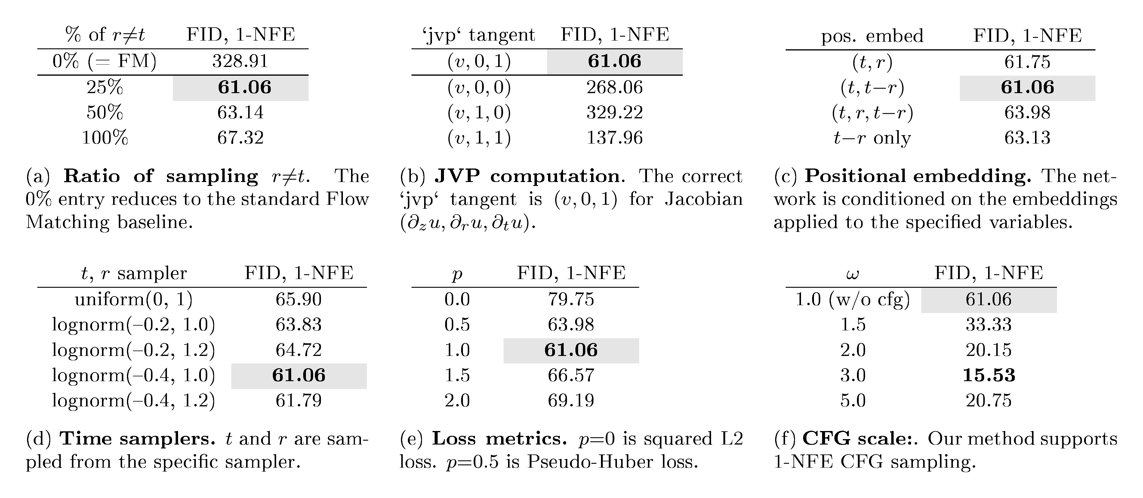
Table 1:Ablation study on 1-NFE ImageNet 256 × 256 generation. FID-50K is evaluated. Default configurations are marked in gray: B/4 backbone, 80-epoch training from scratch.
💭 Click to ask about this figure
From Flow Matching to Mean Flows.
Our method can be viewed as Flow Matching with a modified target (Algorithm 1), and it reduces to standard Flow Matching when rrr always equals ttt. Table 1a compares the ratio of randomly sampling r≠tr \neq tr=t. A 0% ratio of r≠tr \neq tr=t (reducing to Flow Matching) fails to produce reasonable results for 1-NFE generation. A non-zero ratio of r≠tr \neq tr=t enables MeanFlow to take effect, yielding meaningful results under 1-NFE generation. We observe that the model balances between learning the instantaneous velocity (r=tr = tr=t) vs. propagating into r≠tr \neq tr=t via the modified target. Here, the optimal FID is achieved at a ratio of 25%, and a ratio of 100% also yields a valid result.
JVP Computation.
The JVP operation Equation 6 serves as the core relation that connects all (r,t)(r, t)(r,t) coordinates. In Table 1b, we conduct a destructive comparison in which incorrect JVP computation is intentionally performed. It shows that meaningful results are achieved only when the JVP computation is correct. Notably, the JVP tangent along ∂zu\partial_{z}u∂zu is ddd-dimensional, where ddd is the data dimension (here, 32 ×\times× 32 ×\times× 4), and the tangents along ∂ru\partial_{r}u∂ru and ∂tu\partial_{t}u∂tu are one-dimensional. Nevertheless, these two time variables determine the field uuu, and their roles are therefore critical even though they are only one-dimensional.
Conditioning on (r,t)(r, t)(r,t).
As discussed in Section 4.3, we can represent uθ(z,r,t)u_\theta(z, r, t)uθ(z,r,t) by various forms of explicit positional embedding, e.g.,uθ(⋅,r,t)≜net(⋅,t,t−r)u_\theta(\cdot, r, t) \triangleq \texttt{net}(\cdot, t, t-r)uθ(⋅,r,t)≜net(⋅,t,t−r). Table 1c compares these variants. Table 1c shows that all variants of (r,t)(r, t)(r,t) embeddings studied yield meaningful 1-NFE results, demonstrating the effectiveness of MeanFlow as a framework. Embedding (t,t−r)(t, t-r)(t,t−r), that is, time and interval, achieves the best result, while directly embedding (r,t)(r, t)(r,t) performs almost as well. Notably, even embedding only the interval t−rt-rt−r yields reasonable results.
Time Samplers.
Prior work [10] has shown that the distribution used to sample ttt influences the generation quality. We study the distribution used to sample (r,t)(r, t)(r,t) in Table 1d. Note that (r,t)(r, t)(r,t) are first sampled independently, followed by a post-processing step that enforces t>rt > rt>r by swapping and then caps the proportion of r≠tr \neq tr=t to a specified ratio. Table 1d reports that a logit-normal sampler performs the best, consistent with observations on Flow Matching [10].
Loss Metrics.
It has been reported [1] that the choice of loss metrics strongly impacts the performance of few-/one-step generation. We study this aspect in Table 1e. Our loss metric is implemented via adaptive loss weighting [14] with power ppp (Section 4.3). Table 1e shows that p=1p=1p=1 achieves the best result, whereas p=0.5p=0.5p=0.5 (similar to Pseudo-Huber loss [1]) also performs competitively. The standard squared L2 loss (here, p=0p=0p=0) underperforms compared to other settings, but still produces meaningful results, consistent with observations in [1].
Guidance Scale.
Table 1f reports the results with CFG. Consistent with observations in multi-step generation [34], CFG substantially improves generation quality in our 1-NFE setting too. We emphasize that our CFG formulation (Section 4.2) naturally support 1-NFE sampling.
Scalability.
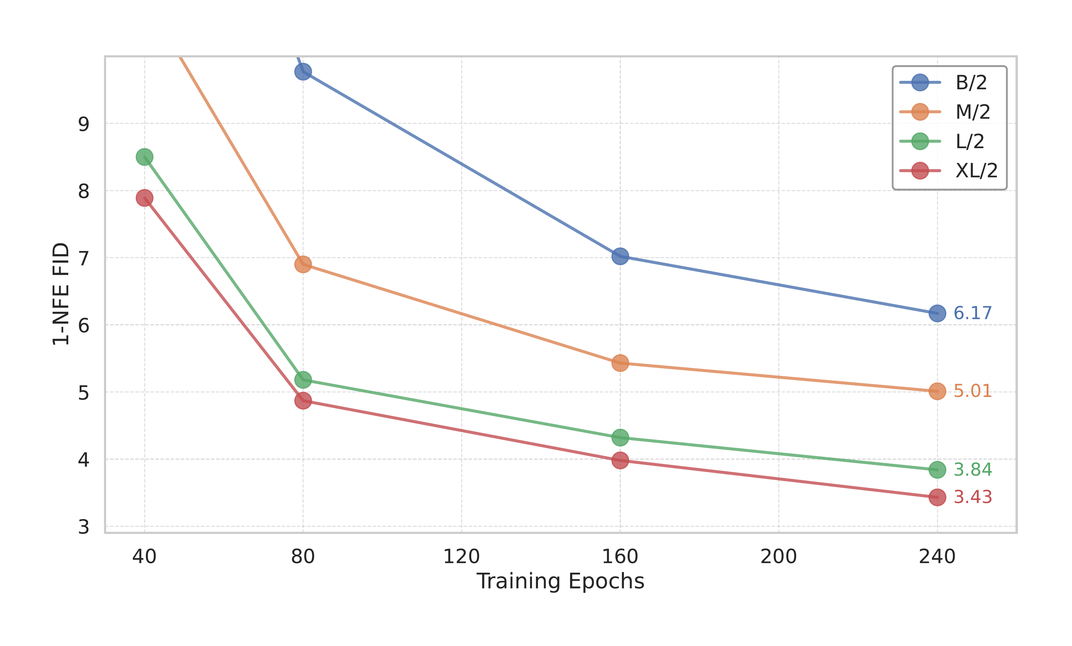
Figure 4 presents the 1-NFE FID results of MeanFlow across larger model sizes and different training durations. Consistent with the behavior of Transformer-based diffusion/flow models (DiT [34] and SiT [11]), MeanFlow models exhibit promising scalability for 1-NFE generation.
5.2 Comparisons with Prior Work
ImageNet 256 ×\times× 256 Comparisons.
In Figure 1 we compare with previous one-step diffusion/flow models, which are also summarized in Table 2 (left). Overall, MeanFlow largely outperforms previous methods in its class: it achieves 3.43 FID, which is an over 50% relative improvement vs. IMM's one-step result of 7.77 [3]; if we compare only 1-NFE (not just one-step) generation, MeanFlow has nearly 70% relative improvement vs. the previous state-of-the-art (10.60, Shortcut [2]). Our method largely closes the gap between one-step and many-step diffusion/flow models.
In 2-NFE generation, our method achieves an FID of 2.20 (Table 2, bottom left). This result is on par with the leading baselines of many-step diffusion/flow models, namely, DiT [34] (FID 2.27) and SiT [11] (FID 2.15), both having an NFE of 250 ×\times× 2 (Table 2, right), under the same XL/2 backbone. Our results suggest that few-step diffusion/flow models can rival their many-step predecessors. Orthogonal improvements, such as REPA [37], are applicable, which are left for future work.
Notably, our method is self-contained and trained entirely from scratch. It achieves the strong results without using any pre-training, distillation, or the curriculum learning adopted in [1, 14, 15].
Figure 4:Scalability of MeanFlow models on ImageNet 256 × 256. 1-NFE generation FID is reported. All models are trained from scratch. CFG is applied while maintaining the 1-NFE sampling behavior. Our method exhibits promising scalability with respect to model size.
💭 Click to ask about this figure
Table 2:Class-conditional generation on ImageNet-256 × 256. All entries are reported with CFG, when applicable. Left: 1-NFE and 2-NFE diffusion/flow models trained from scratch. Right: Other families of generative models as a reference. In both tables, " × 2" indicates that CFG incurs an NFE of 2 per sampling step. Our MeanFlow models are all trained for 240 epochs, except that "MeanFlow-XL+" is trained for more epochs and with configurations selected for longer training, specified in appendix. †: iCT [1] results are reported by [3].
💭 Click to ask about this figure
Table 3:Unconditional CIFAR-10.
method
precond
NFE
FID
iCT [1]
EDM
1
2.83
ECT [14]
EDM
1
3.60
sCT [15]
EDM
1
2.97
CIFAR-10 Comparisons.
We report unconditional generation results on CIFAR-10 [38] (32 ×\times× 32) in Table 3. FID-50K is reported with 1-NFE sampling. All entries are with the same U-net [39] developed from [8] (∼\sim∼ 55M), applied directly on the pixel space. All other competitors are with the EDM-style pre-conditioner [19], and ours has no preconditioner. Implementation details are in the appendix. On this dataset, our method is competitive with prior approaches.
6 Conclusion
Show me a brief summary.
In this section, the authors conclude by positioning MeanFlow as a principled framework for one-step generation that addresses fundamental challenges in multi-scale simulation problems. The work recognizes that numerical simulations in physics are inherently constrained by computational limits in resolving multiple scales across space and time. MeanFlow's approach of describing quantities at coarsened levels of granularity mirrors strategies used in important physics applications, where representing phenomena across different resolutions is essential. By framing generative modeling through this multi-scale lens, the framework establishes connections between generative AI and classical simulation problems in physics and dynamical systems. The authors express hope that this conceptual bridge will foster cross-pollination between these traditionally separate research areas, enabling insights from physics-based simulation to inform generative modeling and vice versa, ultimately advancing both fields through shared mathematical and computational principles.
We have presented MeanFlow, a principled and effective framework for one-step generation. Broadly speaking, the scenario considered in this work is related to multi-scale simulation problems in physics that may involve a range of scales, lengths, and resolution, in space or time. Carrying out numerical simulation is inherently limited by the ability of computers to resolve the range of scales. Our formulation involves describing the underlying quantity at coarsened levels of granularity, a common theme that underlies many important applications in physics. We hope that our work will bridge research in generative modeling, simulation, and dynamical systems in related fields.
Acknowledgement
Show me a brief summary.
In this section, the authors express gratitude to the organizations and individuals who supported their research. Google TPU Research Cloud provided essential computational infrastructure by granting access to TPUs, which were critical for training the large-scale models presented in the work. Financial support came from multiple sources: the Bosch Center for AI funded Zhengyang Geng and Zico Kolter's lab, while the MIT-IBM Watson AI Lab provided funding for Mingyang Deng and Xingjian Bai. Beyond institutional backing, the implementation of the models relied on collaborative technical expertise, with six individuals—Runqian Wang, Qiao Sun, Zhicheng Jiang, Hanhong Zhao, Yiyang Lu, and Xianbang Wang—contributing specifically to the JAX framework and TPU implementation aspects of the project. These combined resources and collaborative efforts enabled the successful development and evaluation of the MeanFlow framework for one-step generative modeling.
We greatly thank Google TPU Research Cloud (TRC) for granting us access to TPUs. Zhengyang Geng is partially supported by funding from the Bosch Center for AI. Zico Kolter gratefully acknowledges Bosch’s funding for the lab. Mingyang Deng and Xingjian Bai are partially supported by the MIT-IBM Watson AI Lab funding award. We thank Runqian Wang, Qiao Sun, Zhicheng Jiang, Hanhong Zhao, Yiyang Lu, and Xianbang Wang for their help on the JAX and TPU implementation.
Appendix
A Implementation
Table 4:Configurations on ImageNet 256 × 256. B/4 is our ablation model.
configs
B/4
B/2
M/2
L/2
XL/2
XL/2+
params (M)
131
131
497.8
459
676
676
FLOPs (G)
5.6
23.1
54.0
119.0
119.0
119.0
depth
12
12
16
24
28
28
hidden dim
768
768
1024
1024
1152
1152
ImageNet 256 ×\times× 256.
We use a standard VAE tokenizer to extract the latent representations3. The latent size is 32 ×\times× 32 ×\times× 4, which is the input to the model. The backbone architectures follow DiT [34], which are based on ViT [36] with adaLN-Zero [34] for conditioning. To condition on two time variables (e.g.,(r,t)(r, t)(r,t)), we apply positional embedding on each time variable, followed by a 2-layer MLP, and summed. We keep the the DiT architecture blocks untouched, while architectural improvements are orthogonal and possible. The configuration specifics are in Table 4.
. We experiment with class-unconditional generation on CIFAR-10. Our implementation follows standard Flow Matching practice [41]. The input to the model is 32 ×\times× 32 ×\times× 3 in the pixel space. The network is a U-net [39] developed from [8] (∼\sim∼ 55M), which is commonly used by other baselines we compare. We apply positional embedding on the two time variables (here, (t,t−r)(t, t-r)(t,t−r)) and concatenate them for conditioning. We do not use any EDM preconditioner [19].
We use Adam with learning rate 0.0006, batch size 1024, (β1,β2)=(0.9,0.999)(\beta_1, \beta_2)=(0.9, 0.999)(β1,β2)=(0.9,0.999), dropout 0.2, weight decay 0, and EMA decay of 0.99995. The model is trained for 800K iterations (with 10K warm-up [42]). The (r,t)(r, t)(r,t) sampler is lognorm(–2.0, 2.0). The ratio of sampling r≠tr \neq tr=t is 75%. The power ppp for adaptive weighting is 0.75. Our data augmentation setup follows [19], with vertical flipping and rotation disabled.
B Additional Technical Details
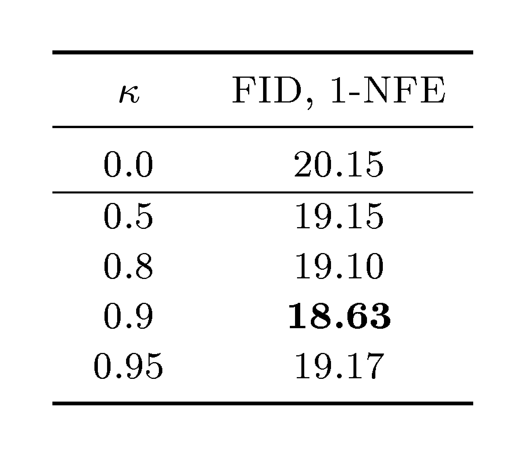
Table 5:Improved CFG for MeanFlow. κ is as defined in Eq. (20), whose goal is to enable both class-conditional ucfg(⋅∣c) and class-unconditional ucfg(⋅) to appear in the target. In this table, we fix the effective guidance scale ω′, given by ω′=ω/(1−κ), as 2.0. Accordingly, for different κ values, we set ω by ω=(1−κ)⋅ω′. If κ=0, it falls back to the CFG case in Eq. (19) (see also Tab. 1f). Similar to standard CFG's practice of randomly dropping class conditions [16], we observe that mixing class-conditional and class-unconditional ucfg in our target improves generation quality.
💭 Click to ask about this figure
B.1 Improved CFG for MeanFlow
In Section 4.2, we have discussed how to naturally extend our method to supporting CFG. The only change needed is to revise the target by Equation 14. We notice that only the class-unconditionalucfgu^\text{cfg}ucfg is presented in Equation 14. In the original CFG [16], it is a standard practice to mix class-conditional and class-unconditional predictions, approached by random dropping. We observe that a similar idea can be applied to our regression target as well.
Formally, we introduce a mixing scale κ\kappaκ and rewrite Equation 12 as:
Here, the role of κ\kappaκ is to mix with ucfg(⋅∣c)u^\text{cfg}(\cdot \mid \mathbf{c})ucfg(⋅∣c) on the right hand side. We can show that Equation 15 satisfies the original CFG formulation Equation (9) with the effective guidance scale of ω′=ω1−κ\omega' = \frac{\omega}{1-\kappa}ω′=1−κω, leveraging the relation v(zt,t)=vcfg(zt,t)v(z_t, t)= v^\text{cfg}(z_t, t)v(zt,t)=vcfg(zt,t) and vcfg(zt,t)=ucfg(zt,t,t)v^\text{cfg}(z_t, t)= u^\text{cfg}(z_t, t, t)vcfg(zt,t)=ucfg(zt,t,t) that we have used for deriving Equation 12. With this, Equation 14 is rewritten as
The loss function is the same as defined in Equation 13.
The influence of introducing κ\kappaκ is explored in Table 5, where we fix the effective guidance scale ω′\omega'ω′ as 2.0 and vary κ\kappaκ. It shows that mixing by κ\kappaκ can further improve generation quality. We note that the ablation in Table 1f in the main paper did not involve this improvement, i.e.,κ\kappaκ was set as 0.
B.2 Loss Metrics
The squared L2 loss is given by L=∥Δ∥22\mathcal{L} = \|\Delta\|^2_2L=∥Δ∥22, where Δ=uθ−utgt\Delta=u_\theta - u_\text{tgt}Δ=uθ−utgt denotes the regression error. Generally, one can adopt the powered L2 loss Lγ=∥Δ∥22γ\mathcal{L}_\gamma = \|\Delta\|^{2\gamma}_2Lγ=∥Δ∥22γ, where γ\gammaγ is a user-specified hyper-parameter. Minimizing this loss is equivalent to minimizing an adaptively weighted squared L2 loss (see [14]): ddθLγ=γ(∥Δ∥22)(γ−1)⋅d∥Δ∥22dθ\frac{d}{d\theta} \mathcal{L}_\gamma = \gamma (\|\Delta\|_2^2)^{(\gamma-1)} \cdot \frac{d\|\Delta\|^{2}_2}{d\theta}dθdLγ=γ(∥Δ∥22)(γ−1)⋅dθd∥Δ∥22. This can be viewed as weighting the squared L2 loss (∥Δ∥22\|\Delta\|^2_2∥Δ∥22) by a loss-adaptive weight λ∝∥Δ∥22(γ−1)\lambda \propto \|\Delta\|_2^{2(\gamma-1)}λ∝∥Δ∥22(γ−1). In practice, we follow [14] and weight by:
w=1/(∥Δ∥22+c)p,
💭 Click to ask about this equation
(22)
where p=1−γp=1-\gammap=1−γ and c>0c>0c>0 is a small constant to avoid division by zero. If p=0.5p=0.5p=0.5, this is similar to the Pseudo-Huber loss in [1]. The adaptively weighted loss is sg(w)⋅L\text{sg}(w)\cdot \mathcal{L}sg(w)⋅L, where sg\text{sg}sg denotes the stop-gradient operator.
B.3 On the Sufficiency of the MeanFlow Identity
In the main paper, starting from the definitional Equation 4, we have derived the MeanFlow Identity Equation 5. This indicates that ``Equation 4 ⇒\Rightarrow⇒ Equation 5", that is, Equation 5 is a necessary condition for Equation 4. Next, we show that it is also a sufficient condition, that is, "Equation 5 ⇒\Rightarrow⇒ Equation 4".
In general, equality of derivatives does not imply equality of integrals: they may differ by a constant. In our case, we show that the constant is canceled out. Consider a "displacement field" SSS written as:
S(zt,r,t)=(t−r)u(zt,r,t).
💭 Click to ask about this equation
(23)
If we treat SSS as an arbitrary function, then in general, equality of derivatives can only lead to equality of integrals, up to some constants:
However, the definition of SSS gives S∣t=r=0S|_{t=r}=0S∣t=r=0, and we also have ∫rtvdτ=0\int_{r}^{t}vd\tau=0∫rtvdτ=0 when t=rt=rt=r, which gives C1=C2C_1 = C_2C1=C2. This indicates "Equation 5 ⇒\Rightarrow⇒ Equation 4".
We note that this sufficiency is a consequence of modeling the average velocity uuu, rather than directly the displacement SSS. Enforcing the equality of derivatives on the displacement, for example, ddtS=v\frac{d}{d t}{S}=vdtdS=v, does not automatically yield S=∫rtvdτS=\int^t_r v d\tauS=∫rtvdτ. If we were to parameterize SSS directly, an extra boundary condition S∣t=r=0S |_{t=r} = 0S∣t=r=0 is needed. Our formulation can automatically satisfy this condition.
B.4 Analysis on Jacobian-Vector Product (JVP) Computation
While JVP computation can be seen as a concern in some methods, it is very lightweight in ours. In our case, as the computed product (between the Jacobian matrix and the tangent vector) is subject to stop-gradient Equation (7b), it is treated as a constant when conducting SGD using backpropagation w.r.t.θ\thetaθ. Consequently, it does not add any overhead to the θ\thetaθ-backpropagation.
As such, the extra computation incurred by computing this product is the ``backward" pass performed by the jvp operation. This backward is analogous to the standard backward pass used for optimizing neural networks (w.r.t.θ\thetaθ)—in fact, in some deep learning libraries, such as JAX [43], they use similar interfaces to compute the standard backpropagation (w.r.t.θ\thetaθ). In our case, it is even less costly than a standard backpropagation, as it only needs to backpropagate to the input variables, not to the parameters θ\thetaθ. This overhead is small.
We benchmark the overhead caused by JVP in our ablation model, B/4. We implement the model in JAX and benchmark in v4-8 TPUs. We compare MeanFlow with its Flow Matching counterpart, where the only overhead is the backward pass incurred by JVP; notice that the forward pass of JVP is the standard forward propagation, which Flow Matching (or any typical objective function) also needs to perform. In our benchmarking, the training cost is 0.045 sec/iter using Flow Matching, and 0.052 sec/iter using MeanFlow, which is a merely 16% wall-clock overhead.
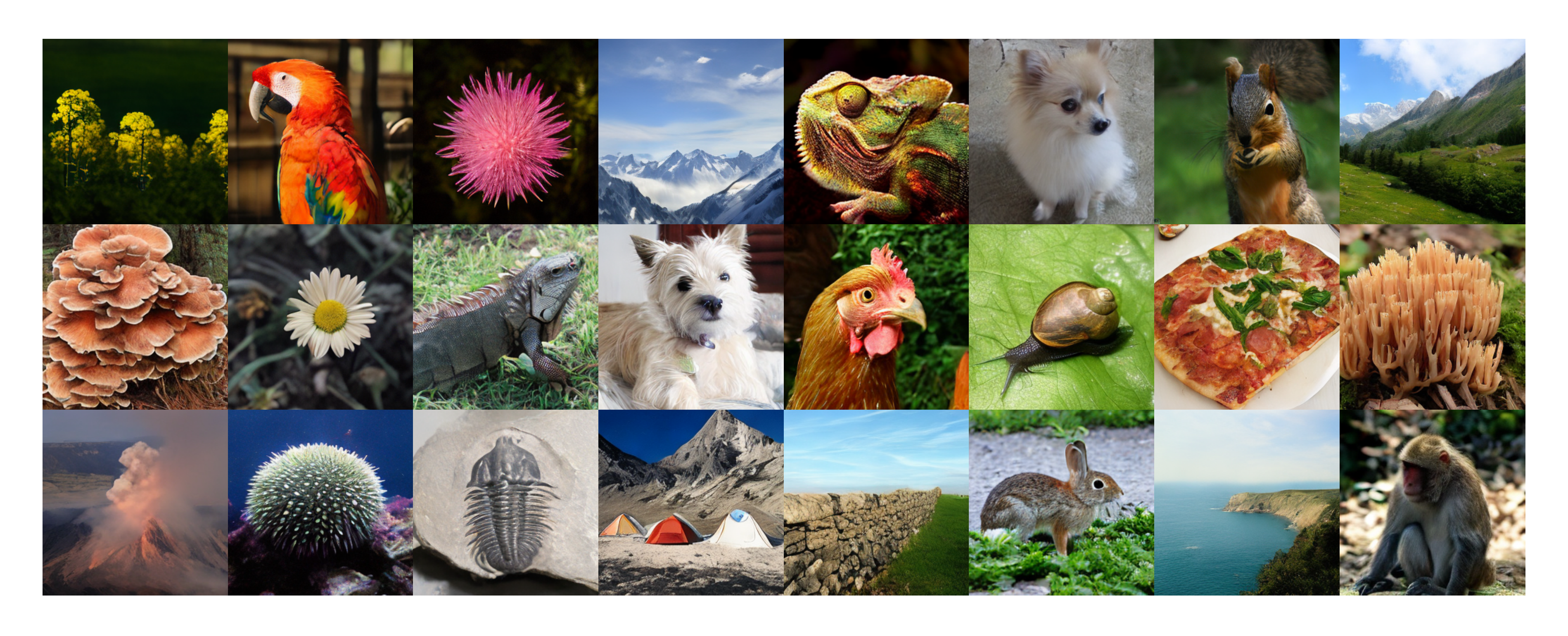
Figure 5:1-NFE Generation Results. We show curated examples of class-conditional generation on ImageNet 256 × 256 using our 1-NFE model (MeanFlow-XL/2, 3.43 FID).
💭 Click to ask about this figure
C Qualitative Results
Figure 5 shows curated generation examples on ImageNet 256 ×\times× 256 using our 1-NFE model.
References
Show me a brief summary.
In this section, the references catalog the foundational and contemporary work underpinning MeanFlow's development in generative modeling. The citations span core diffusion and flow matching techniques, including seminal papers on denoising diffusion probabilistic models, score-based generative modeling, and flow matching frameworks that establish the theoretical basis for continuous-time generative processes. Key distillation methods like consistency models, progressive distillation, and distribution matching are referenced as approaches to accelerate sampling from pretrained models. The list includes architectural foundations such as Vision Transformers and U-Nets, optimization techniques like Adam, and practical training strategies for large-scale image synthesis. References to ImageNet and CIFAR-10 datasets ground the empirical evaluation context. Implementation tools, particularly JAX for automatic differentiation and TPU computation, are acknowledged. Together, these works form the ecosystem within which MeanFlow operates, positioning it as an advancement that achieves single-step generation while maintaining competitive quality through its novel average velocity formulation.
[1] Yang Song and Prafulla Dhariwal. Improved techniques for training consistency models. In International Conference on Learning Representations (ICLR), 2024.
[2] Kevin Frans, Danijar Hafner, Sergey Levine, and Pieter Abbeel. One step diffusion via shortcut models. In International Conference on Learning Representations (ICLR), 2025.
[3] Linqi Zhou, Stefano Ermon, and Jiaming Song. Inductive moment matching. arXiv preprint arXiv:2503.07565, 2025.
[4] Yaron Lipman, Ricky T. Q. Chen, Heli Ben-Hamu, Maximilian Nickel, and Matthew Le. Flow matching for generative modeling. In International Conference on Learning Representations (ICLR), 2023.
[5] Michael Samuel Albergo and Eric Vanden-Eijnden. Building normalizing flows with stochastic interpolants. In International Conference on Learning Representations (ICLR), 2023.
[6] Xingchao Liu, Chengyue Gong, and qiang liu. Flow straight and fast: Learning to generate and transfer data with rectified flow. In International Conference on Learning Representations (ICLR), 2023.
[7] Jascha Sohl-Dickstein, Eric Weiss, Niru Maheswaranathan, and Surya Ganguli. Deep unsupervised learning using nonequilibrium thermodynamics. In International Conference on Machine Learning (ICML), 2015.
[8] Yang Song and Stefano Ermon. Generative modeling by estimating gradients of the data distribution. Neural Information Processing Systems (NeurIPS), 2019.
[9] Jonathan Ho, Ajay Jain, and Pieter Abbeel. Denoising diffusion probabilistic models. Neural Information Processing Systems (NeurIPS), 2020.
[10] Patrick Esser, Sumith Kulal, Andreas Blattmann, Rahim Entezari, Jonas Müller, Harry Saini, Yam Levi, Dominik Lorenz, Axel Sauer, Frederic Boesel, et al. Scaling rectified flow transformers for high-resolution image synthesis. In Forty-first international conference on machine learning, 2024.
[11] Nanye Ma, Mark Goldstein, Michael S Albergo, Nicholas M Boffi, Eric Vanden-Eijnden, and Saining Xie. Sit: Exploring flow and diffusion-based generative models with scalable interpolant transformers. In European Conference on Computer Vision (ECCV), 2024.
[12] Adam Polyak, , et al. Movie Gen: A cast of media foundation models, 2025.
[13] Yang Song, Prafulla Dhariwal, Mark Chen, and Ilya Sutskever. Consistency models. In International Conference on Machine Learning (ICML), 2023.
[14] Zhengyang Geng, Ashwini Pokle, William Luo, Justin Lin, and J Zico Kolter. Consistency models made easy. arXiv preprint arXiv:2406.14548, 2024.
[15] Cheng Lu and Yang Song. Simplifying, stabilizing and scaling continuous-time consistency models. In International Conference on Learning Representations (ICLR), 2025.
[16] Jonathan Ho and Tim Salimans. Classifier-free diffusion guidance. arXiv preprint arXiv:2207.12598, 2022.
[17] Jia Deng, Wei Dong, Richard Socher, Li-Jia Li, Kai Li, and Li Fei-Fei. Imagenet: A large-scale hierarchical image database. In IEEE Conference on Computer Vision and Pattern Recognition (CVPR), 2009.
[18] Yang Song, Jascha Sohl-Dickstein, Diederik P Kingma, Abhishek Kumar, Stefano Ermon, and Ben Poole. Score-based generative modeling through stochastic differential equations. In International Conference on Learning Representations (ICLR), 2021.
[19] Tero Karras, Miika Aittala, Timo Aila, and Samuli Laine. Elucidating the design space of diffusion-based generative models. In Neural Information Processing Systems (NeurIPS), 2022.
[20] Danilo Rezende and Shakir Mohamed. Variational inference with normalizing flows. In International Conference on Machine Learning (ICML), 2015.
[21] Tim Salimans and Jonathan Ho. Progressive distillation for fast sampling of diffusion models. In International Conference on Learning Representations (ICLR), 2022.
[22] Zhengyang Geng, Ashwini Pokle, and J Zico Kolter. One-step diffusion distillation via deep equilibrium models. Neural Information Processing Systems (NeurIPS), 36, 2024.
[23] Axel Sauer, Dominik Lorenz, Andreas Blattmann, and Robin Rombach. Adversarial diffusion distillation. In European Conference on Computer Vision (ECCV), 2024.
[24] Weijian Luo, Tianyang Hu, Shifeng Zhang, Jiacheng Sun, Zhenguo Li, and Zhihua Zhang. Diff-instruct: A universal approach for transferring knowledge from pre-trained diffusion models. Neural Information Processing Systems (NeurIPS), 2024.
[25] Tianwei Yin, Michaël Gharbi, Richard Zhang, Eli Shechtman, Frédo Durand, William T Freeman, and Taesung Park. One-step diffusion with distribution matching distillation. In IEEE Conference on Computer Vision and Pattern Recognition (CVPR), 2024.
[26] Mingyuan Zhou, Huangjie Zheng, Zhendong Wang, Mingzhang Yin, and Hai Huang. Score identity distillation: Exponentially fast distillation of pretrained diffusion models for one-step generation. In International Conference on Machine Learning (ICML), 2024.
[30] Michael S Albergo and Eric Vanden-Eijnden. Building normalizing flows with stochastic interpolants. arXiv preprint arXiv:2209.15571, 2022.
[31] Dongjun Kim, Chieh-Hsin Lai, Wei-Hsiang Liao, Naoki Murata, Yuhta Takida, Toshimitsu Uesaka, Yutong He, Yuki Mitsufuji, and Stefano Ermon. Consistency trajectory models: Learning probability flow ODE trajectory of diffusion. In International Conference on Learning Representations (ICLR), 2024.
[32] Ashish Vaswani, Noam Shazeer, Niki Parmar, Jakob Uszkoreit, Llion Jones, Aidan N Gomez, Lukasz Kaiser, and Illia Polosukhin. Attention is all you need. Neural Information Processing Systems (NeurIPS), 2017.
[33] Martin Heusel, Hubert Ramsauer, Thomas Unterthiner, Bernhard Nessler, and Sepp Hochreiter. Gans trained by a two time-scale update rule converge to a local nash equilibrium. Neural Information Processing Systems (NeurIPS), 2017.
[34] William Peebles and Saining Xie. Scalable diffusion models with transformers. In IEEE Conference on Computer Vision and Pattern Recognition (CVPR), 2023.
[35] Robin Rombach, Andreas Blattmann, Dominik Lorenz, Patrick Esser, and Björn Ommer. High-resolution image synthesis with latent diffusion models. In IEEE Conference on Computer Vision and Pattern Recognition (CVPR), 2021.
[36] Alexey Dosovitskiy, Lucas Beyer, Alexander Kolesnikov, Dirk Weissenborn, Xiaohua Zhai, Thomas Unterthiner, Mostafa Dehghani, Matthias Minderer, Georg Heigold, Sylvain Gelly, Jakob Uszkoreit, and Neil Houlsby. An image is worth 16x16 words: Transformers for image recognition at scale. In International Conference on Learning Representations (ICLR), 2021.
[37] Sihyun Yu, Sangkyung Kwak, Huiwon Jang, Jongheon Jeong, Jonathan Huang, Jinwoo Shin, and Saining Xie. Representation alignment for generation: Training diffusion transformers is easier than you think. In International Conference on Learning Representations (ICLR), 2025.
[39] Olaf Ronneberger, Philipp Fischer, and Thomas Brox. U-net: Convolutional networks for biomedical image segmentation. In Medical image computing and computer-assisted intervention (MICCAI), 2015.
[40] Diederik P. Kingma and Jimmy Ba. Adam: A method for stochastic optimization. In International Conference on Learning Representations (ICLR), 2015.
[41] Yaron Lipman, Marton Havasi, Peter Holderrieth, Neta Shaul, Matt Le, Brian Karrer, Ricky T. Q. Chen, David Lopez-Paz, Heli Ben-Hamu, and Itai Gat. Flow matching guide and code, 2024. URL https://arxiv.org/abs/2412.06264.
[42] Priya Goyal, Piotr Dollár, Ross Girshick, Pieter Noordhuis, Lukasz Wesolowski, Aapo Kyrola, Andrew Tulloch, Yangqing Jia, and Kaiming He. Accurate, large minibatch sgd: Training imagenet in 1 hour. arXiv preprint arXiv:1706.02677, 2017.
[43] James Bradbury, Roy Frostig, Peter Hawkins, Matthew James Johnson, Chris Leary, Dougal Maclaurin, George Necula, Adam Paszke, Jake VanderPlas, Skye Wanderman-Milne, and Qiao Zhang. JAX: composable transformations of Python+NumPy programs, 2018. URL http://github.com/google/jax.
![**Figure 1:** **One-step generation on ImageNet 256 $\times$ 256 from scratch**. Our *MeanFlow* (**MF**) model achieves significantly better generation quality than previous state-of-the-art one-step diffusion/flow methods. Here, iCT [1], Shortcut [2], and our MF are all **1-NFE** generation, while IMM's 1-step result [3] involves 2-NFE guidance. Detailed numbers are in Tab. 2. Images shown are generated by our 1-NFE model.](https://ittowtnkqtyixxjxrhou.supabase.co/storage/v1/object/public/public-images/cva77gew/complex_fig_2cf67d9b93dc.png)
![**Figure 2:** **Velocity fields in Flow Matching** [4]. **Left**: *conditional* flows [4]. A given $z_t$ can arise from different $(x, {\epsilon})$ pairs, resulting in different conditional velocities $v_t$. **Right**: *marginal* flows [4], obtained by marginalizing over all possible conditional velocities. The marginal velocity field serves as the underlying ground-truth field for network training. All velocities shown here are essentially *instantaneous* velocities. Illustration follows [29]. (*Gray dots: samples from prior; red dots: samples from data.*)](https://ittowtnkqtyixxjxrhou.supabase.co/storage/v1/object/public/public-images/cva77gew/complex_fig_5a75b9b5816f.png)