Equivariant Diffusion for Molecule Generation in 3D

Emiel HoogeboomVictor Garcia SatorrasClément VignacMax Welling

article2022ICML847 citations

Introduces an E(3) equivariant diffusion model that jointly generates 3D atomic coordinates and discrete atom types while enabling exact likelihood computation, outperforming existing molecular generative methods in quality and training speed.

Listen

Designing novel molecules directly in three-dimensional space is essential for computational drug discovery and materials design, yet existing generative artificial intelligence approaches face major bottlenecks. Prior methods either require imposing an artificial, step-by-step ordering on atoms or rely on continuous flow techniques that are computationally expensive to train and difficult to scale to large structures. Moreover, molecular generation models must inherently respect natural geometric symmetries—such as rotations, reflections, and translations—to generalize accurately in real physical systems.

The main objective of the article is to introduce and evaluate an Equivariant Diffusion Model, a generative system that directly produces 3D molecular coordinates and discrete atom properties simultaneously while strictly preserving 3D geometric symmetries. The authors demonstrate the model's ability to generate chemically realistic molecules, establish a rigorous probabilistic framework to compute exact sample likelihoods, and extend the model to target specific desired chemical properties.

To accomplish this, the authors designed a diffusion-based denoising process that jointly treats continuous 3D atomic coordinates and discrete categorical atom types. The core neural architecture utilizes equivariant graph networks that automatically maintain geometric consistency regardless of how a molecule is rotated or translated in space. The approach was evaluated on standard computational chemistry benchmarks: the QM9 dataset comprising 130,000 small molecules, and the GEOM-Drugs dataset containing larger, drug-like molecular conformations averaging over 44 atoms per structure.

The experimental findings show significant improvements across all key benchmarks. On the QM9 dataset, the proposed model achieved an 82.0% molecular stability rate, vastly outperforming previous geometric flow models (4.9%) and autoregressive baselines (68.1%), while cutting training time in half compared to flow-based methods. When evaluated on chemical validity and uniqueness with explicit hydrogen atoms, the model reached 90.7%, compared to 39.4% for prior flow models and 80.3% for autoregressive baselines. On the larger GEOM-Drugs benchmark, the model produced superior atom stability (81.3%) and accurately matched the dataset's energy distributions, whereas non-geometric variants generated unrealistic low-energy states. Furthermore, conditional experiments confirmed that the model successfully guided structural generation according to targeted physical properties such as polarizability and orbital energy gaps.

These findings indicate that equivariant diffusion offers a significantly more scalable and physically coherent foundation for computer-aided molecular design. By eliminating the need for expensive differential equation solvers or arbitrary atom orderings, the framework reduces computational overhead while dramatically boosting structural fidelity. This reduces the risk of generating chemically infeasible candidate structures during early-stage discovery pipelines, accelerating timelines for identifying viable drug candidates.

Organizations developing computational chemistry pipelines should consider adopting equivariant diffusion frameworks over legacy autoregressive or normalizing flow architectures. Future work should focus on implementing accelerated sampling techniques to reduce generation times during deployment and testing the model on complex macro-molecular and protein-ligand binding tasks.

The reported results have high credibility across standard benchmark datasets, supported by rigorous mathematical proofs of invariance and consistent empirical baselines. However, decision-makers should note certain limitations: sampling can take several seconds per molecule without downstream sampling optimizations, and on very large drug structures, the model occasionally produces disconnected molecular fragments or oversized rings due to the absence of explicit structural regularization.

Cover for Equivariant Diffusion for Molecule Generation in 3D

Abstract

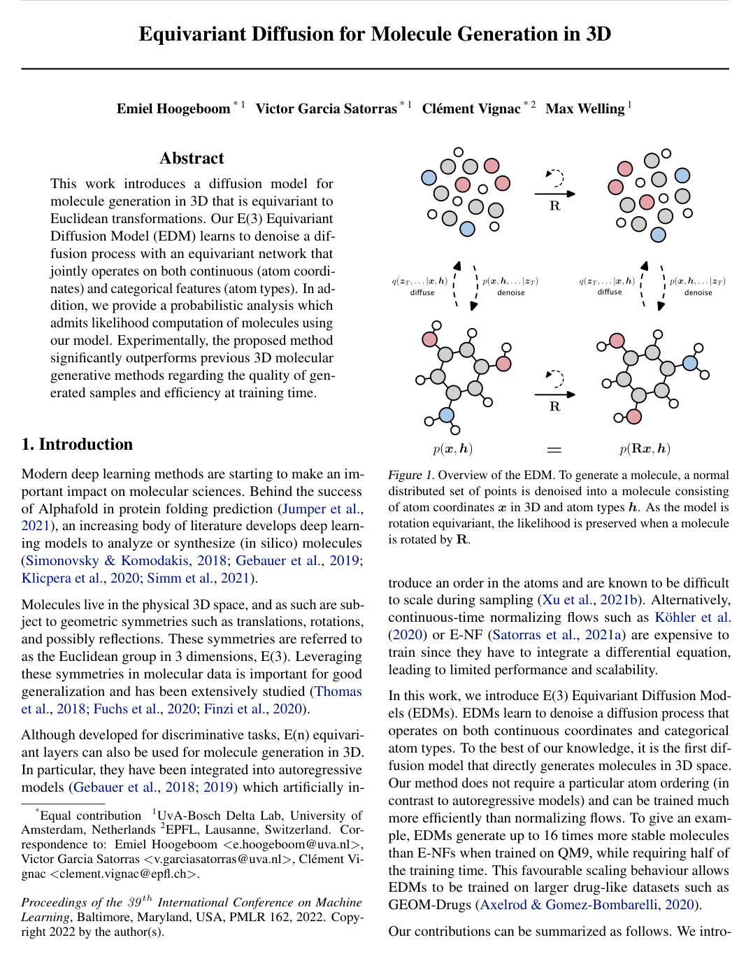
This work introduces a diffusion model for molecule generation in 3D that is equivariant to Euclidean transformations. Our E(3) Equivariant Diffusion Model (EDM) learns to denoise a diffusion process with an equivariant network that jointly operates on both continuous (atom coordinates) and categorical features (atom types). In addition, we provide a probabilistic analysis which admits likelihood computation of molecules using our model. Experimentally, the proposed method significantly outperforms previous 3D molecular generative methods regarding the quality of generated samples and efficiency at training time.

Table of Contents

  • 1 Introduction
  • 2 Background
  • 2.1 Diffusion Models
  • 2.2 Equivariance
  • 3 EDM: E(3) Equivariant Diffusion Model
  • 3.1 The Diffusion Process
  • 3.2 The Dynamics
  • 3.3 The Zeroth Likelihood Term
  • 3.4 Conditional generation
  • 4 Related Work
  • 5 Experiments
  • 5.1 Molecule Generation — QM9
  • 5.2 Conditional Molecule Generation
  • 5.3 GEOM-Drugs
  • 6 Conclusions
  • References
  • A The zero center of gravity, normal distribution
  • B Additional Details for the Method
  • C Additional Details on Experiments
  • D Samples from our models
  • E Conditional generation

Knowls

  1. Knowl 1 — E(3) Equivariant Diffusion Model for 3D Molecule Generation

    model/method

    The E(3) Equivariant Diffusion Model (EDM) directly generates 3D molecular structures by learning to invert a continuous diffusion process defined jointly over 3D atom coordinates and categorical/ordinal atom features without imposing an artificial atom ordering.

    A molecule with MM atoms is represented by spatial coordinates x=(x1,…,xM)∈RM×3\mathbf{x} = (\mathbf{x}_1, \dots, \mathbf{x}_M) \in \mathbb{R}^{M \times 3} and atom features h=(h1,…,hM)∈RM×nf\mathbf{h} = (\mathbf{h}_1, \dots, \mathbf{h}_M) \in \mathbb{R}^{M \times n_f} (e.g., one-hot atom types and integer charges). The forward diffusion process adds Gaussian noise to the concatenated state zt=[zt(x),zt(h)]\mathbf{z}_t = [\mathbf{z}_t^{(x)}, \mathbf{z}_t^{(h)}] across discrete time steps t∈{0,…,T}t \in \{0, \dots, T\} according to:

    q(zt∣x,h)=Nx(zt(x)∣αtx,σt2I)⋅N(zt(h)∣αth,σt2I)q(\mathbf{z}_t \mid \mathbf{x}, \mathbf{h}) = \mathcal{N}_x(\mathbf{z}_t^{(x)} \mid \alpha_t \mathbf{x}, \sigma_t^2 \mathbf{I}) \cdot \mathcal{N}(\mathbf{z}_t^{(h)} \mid \alpha_t \mathbf{h}, \sigma_t^2 \mathbf{I})

    where αt,σt∈R+\alpha_t, \sigma_t \in \mathbb{R}^+ are variance-preserving noise schedule parameters satisfying αt=1−σt2\alpha_t = \sqrt{1 - \sigma_t^2} with α0≈1\alpha_0 \approx 1 and αT≈0\alpha_T \approx 0. To ensure translation invariance, coordinates x\mathbf{x} and coordinate latent variables zt(x)\mathbf{z}_t^{(x)} are constrained to the linear subspace where the center of gravity is zero (∑i=1Mxi=0\sum_{i=1}^M \mathbf{x}_i = \mathbf{0}), represented by distribution Nx\mathcal{N}_x. The generative reverse process p(zs∣zt)p(\mathbf{z}_{s} \mid \mathbf{z}_t) (for s=t−1s = t-1) is parameterized by an equivariant neural network ϕ\phi that predicts the noise ϵ^t=ϕ(zt,t)\hat{\boldsymbol{\epsilon}}_t = \phi(\mathbf{z}_t, t) to reconstruct the denoised molecule [x^,h^]=zt/αt−ϵ^tσt/αt[\hat{\mathbf{x}}, \hat{\mathbf{h}}] = \mathbf{z}_t / \alpha_t - \hat{\boldsymbol{\epsilon}}_t \sigma_t / \alpha_t.

  2. Knowl 2 — Coordinate Diffusion on the Zero Center-of-Gravity Linear Subspace

    theoretical result

    Because a non-zero probability distribution over RM×n\mathbb{R}^{M \times n} (n=3n=3) cannot be strictly translation invariant while integrating to 1, molecular coordinates x∈RM×n\mathbf{x} \in \mathbb{R}^{M \times n} are restricted to the (M−1)n(M-1)n-dimensional linear subspace defined by a zero center of gravity, ∑i=1Mxi=0\sum_{i=1}^M \mathbf{x}_i = \mathbf{0}. Over this subspace, the normal distribution Nx\mathcal{N}_x with mean μ\boldsymbol{\mu} in the subspace and isotropic variance σ2I\sigma^2 \mathbf{I} has density:

    Nx(x∣μ,σ2I)=(2πσ)−(M−1)nexp⁡(−12σ2∥x−μ∥2)\mathcal{N}_x(\mathbf{x} \mid \boldsymbol{\mu}, \sigma^2 \mathbf{I}) = (\sqrt{2\pi}\sigma)^{-(M-1)n} \exp\left(-\frac{1}{2\sigma^2}\|\mathbf{x} - \boldsymbol{\mu}\|^2\right)

    For two distributions q=Nx(μ1,σ2I)q = \mathcal{N}_x(\boldsymbol{\mu}_1, \sigma^2 \mathbf{I}) and p=Nx(μ2,σ2I)p = \mathcal{N}_x(\boldsymbol{\mu}_2, \sigma^2 \mathbf{I}) with identical variance σ2\sigma^2 on this subspace, an orthogonal transformation QQ that projects the zero-mean ambient space to the subspace preserves the Euclidean norm (i.e., ∥μ~1−μ~2∥2=∥μ1−μ2∥2\|\tilde{\boldsymbol{\mu}}_1 - \tilde{\boldsymbol{\mu}}_2\|^2 = \|\boldsymbol{\mu}_1 - \boldsymbol{\mu}_2\|^2). Consequently, the Kullback-Leibler divergence simplifies to:

    KL(q∥p)=12σ2∥μ1−μ2∥2\mathrm{KL}(q \parallel p) = \frac{1}{2\sigma^2} \|\boldsymbol{\mu}_1 - \boldsymbol{\mu}_2\|^2

    Because the coordinate subspace distribution Nx\mathcal{N}_x and feature distribution N\mathcal{N} are independent and isotropic with matching variances, their joint divergence factors and computes identically in ambient space by vector concatenation: KL(Nxh(μ1,σ2I)∥Nxh(μ2,σ2I))=12σ2∥μ1−μ2∥2\mathrm{KL}(\mathcal{N}_{xh}(\boldsymbol{\mu}_1, \sigma^2 \mathbf{I}) \parallel \mathcal{N}_{xh}(\boldsymbol{\mu}_2, \sigma^2 \mathbf{I})) = \frac{1}{2\sigma^2} \|\boldsymbol{\mu}_1 - \boldsymbol{\mu}_2\|^2 for μ=[μ(x),μ(h)]\boldsymbol{\mu} = [\boldsymbol{\mu}^{(x)}, \boldsymbol{\mu}^{(h)}].

  3. Knowl 3 — Equivariant Denoising Network Parameterization using EGNN

    model/method

    The noise prediction function [ϵ^t(x),ϵ^t(h)]=ϕ(zt(x),zt(h),t)[\hat{\boldsymbol{\epsilon}}_t^{(x)}, \hat{\boldsymbol{\epsilon}}_t^{(h)}] = \phi(\mathbf{z}_t^{(x)}, \mathbf{z}_t^{(h)}, t) is parameterized by an E(n)E(n) Equivariant Graph Neural Network (EGNN) operating on a fully connected graph across all MM atoms.

    The input to EGNN is the coordinate matrix zt(x)∈RM×3\mathbf{z}_t^{(x)} \in \mathbb{R}^{M \times 3} and node feature matrix [zt(h),t/T]∈RM×(nf+1)[\mathbf{z}_t^{(h)}, t/T] \in \mathbb{R}^{M \times (n_f + 1)}. The EGNN consists of LL Equivariant Graph Convolutional Layers (EGCL), where layer ll updates messages mij\mathbf{m}_{ij}, node embeddings hil\mathbf{h}_i^l, and coordinates xil\mathbf{x}_i^l via:

    mij=ϕe(hil,hjl,dij2,aij)\mathbf{m}_{ij} = \phi_e\left(\mathbf{h}_i^l, \mathbf{h}_j^l, d_{ij}^2, a_{ij}\right)

    e~ij=ϕinf(mij)\tilde{e}_{ij} = \phi_{\mathrm{inf}}(\mathbf{m}_{ij})

    hil+1=ϕh(hil,∑j≠ie~ijmij)\mathbf{h}_i^{l+1} = \phi_h\left(\mathbf{h}_i^l, \sum_{j \neq i} \tilde{e}_{ij} \mathbf{m}_{ij}\right)

    xil+1=xil+∑j≠ixil−xjldij+1ϕx(hil,hjl,dij2,aij)\mathbf{x}_i^{l+1} = \mathbf{x}_i^l + \sum_{j \neq i} \frac{\mathbf{x}_i^l - \mathbf{x}_j^l}{d_{ij} + 1} \phi_x\left(\mathbf{h}_i^l, \mathbf{h}_j^l, d_{ij}^2, a_{ij}\right)

    where dij=∥xil−xjl∥2d_{ij} = \|\mathbf{x}_i^l - \mathbf{x}_j^l\|_2, aij=∥xi0−xj0∥22a_{ij} = \|\mathbf{x}_i^0 - \mathbf{x}_j^0\|_2^2 is the initial squared distance, ϕinf\phi_{\mathrm{inf}} is a soft edge attention mechanism, and ϕe,ϕh,ϕx\phi_e, \phi_h, \phi_x are multilayer perceptrons. The coordinate noise estimate is computed as xL−zt(x)\mathbf{x}^L - \mathbf{z}_t^{(x)}, and then projected onto the zero center-of-gravity subspace by subtracting its centroid: ϵ^t(x)←ϵ^t(x)−1M∑i=1Mϵ^t,i(x)\hat{\boldsymbol{\epsilon}}_t^{(x)} \leftarrow \hat{\boldsymbol{\epsilon}}_t^{(x)} - \frac{1}{M}\sum_{i=1}^M \hat{\boldsymbol{\epsilon}}_{t, i}^{(x)}. This guarantees that predicted coordinates x^\hat{\mathbf{x}} transform equivariantly under rotations and reflections R∈O(3)\mathbf{R} \in \mathrm{O}(3) and translations.

  4. Knowl 4 — Reconstruction Likelihood and Zeroth Loss Term for Discrete and Continuous Features

    equation

    In the variational lower bound of the Equivariant Diffusion Model, the zeroth data reconstruction term L0=log⁡p(x,h∣z0)=L0(x)+L0(h)\mathcal{L}_0 = \log p(\mathbf{x}, \mathbf{h} \mid \mathbf{z}_0) = \mathcal{L}_0^{(x)} + \mathcal{L}_0^{(h)} is defined separately for continuous coordinates and discrete features:

    1. Continuous coordinates x∈RM×3\mathbf{x} \in \mathbb{R}^{M \times 3}: Under coordinate denoising mean prediction x^=z0(x)/α0−(σ0/α0)ϵ^0(x)\hat{\mathbf{x}} = \mathbf{z}_0^{(x)}/\alpha_0 - (\sigma_0/\alpha_0)\hat{\boldsymbol{\epsilon}}_0^{(x)}, the conditional distribution is p(x∣z0)=Nx(x∣z0(x)/α0−(σ0/α0)ϵ^0(x),(σ02/α02)I)p(\mathbf{x} \mid \mathbf{z}_0) = \mathcal{N}_x(\mathbf{x} \mid \mathbf{z}_0^{(x)}/\alpha_0 - (\sigma_0/\alpha_0)\hat{\boldsymbol{\epsilon}}_0^{(x)}, (\sigma_0^2/\alpha_0^2)\mathbf{I}), resulting in:

    L0(x)=Eϵ(x)∼Nx(0,I)[−log⁡Z−12∥ϵ(x)−ϕ(x)(z0,0)∥2]\mathcal{L}_0^{(x)} = \mathbb{E}_{\boldsymbol{\epsilon}^{(x)} \sim \mathcal{N}_x(\mathbf{0}, \mathbf{I})} \left[ -\log Z - \frac{1}{2} \|\boldsymbol{\epsilon}^{(x)} - \phi^{(x)}(\mathbf{z}_0, 0)\|^2 \right]

    where Z=(2π⋅σ0/α0)(M−1)nZ = (\sqrt{2\pi} \cdot \sigma_0 / \alpha_0)^{(M-1)n} is the normalization constant for spatial dimension n=3n=3.

    1. Categorical features (one-hot encoded atom types honehot\mathbf{h}^{\mathrm{onehot}}): Decoded via a categorical distribution C(h∣p)\mathcal{C}(\mathbf{h} \mid \mathbf{p}) with probabilities defined by integrating the normal density over a unit interval around 1:

    p(h∣z0(h))=C(h∣p),p∝∫1−1/21+1/2N(u∣z0(h),σ0) du=Φ(3/2−z0(h)σ0)−Φ(1/2−z0(h)σ0)p(\mathbf{h} \mid \mathbf{z}_0^{(h)}) = \mathcal{C}(\mathbf{h} \mid \mathbf{p}), \quad \mathbf{p} \propto \int_{1 - 1/2}^{1 + 1/2} \mathcal{N}(u \mid \mathbf{z}_0^{(h)}, \sigma_0) \, du = \Phi\left(\frac{3/2 - \mathbf{z}_0^{(h)}}{\sigma_0}\right) - \Phi\left(\frac{1/2 - \mathbf{z}_0^{(h)}}{\sigma_0}\right)

    where Φ\Phi is the standard normal cumulative distribution function and p\mathbf{p} is normalized to sum to 1.

    1. Integer/ordinal features (atom charge hh):

    p(h∣z0(h))=∫h−1/2h+1/2N(u∣z0(h),σ0) du=Φ(h+1/2−z0(h)σ0)−Φ(h−1/2−z0(h)σ0)p(h \mid z_0^{(h)}) = \int_{h - 1/2}^{h + 1/2} \mathcal{N}(u \mid z_0^{(h)}, \sigma_0) \, du = \Phi\left(\frac{h + 1/2 - z_0^{(h)}}{\sigma_0}\right) - \Phi\left(\frac{h - 1/2 - z_0^{(h)}}{\sigma_0}\right)

  5. Knowl 5 — Invariance Preservation under Equivariant Denoising Markov Chains

    theoretical result

    Let zT∼p(zT)=N(0,I)\mathbf{z}_T \sim p(\mathbf{z}_T) = \mathcal{N}(\mathbf{0}, \mathbf{I}) be an initial latent state distribution that is invariant under orthogonal group actions R∈O(3)\mathbf{R} \in \mathrm{O}(3), such that p(RzT)=p(zT)p(\mathbf{R}\mathbf{z}_T) = p(\mathbf{z}_T). If each reverse Markov transition kernel p(zt−1∣zt)p(\mathbf{z}_{t-1} \mid \mathbf{z}_t) is equivariant to orthogonal transformations:

    p(zt−1∣zt)=p(Rzt−1∣Rzt)∀R∈O(3)p(\mathbf{z}_{t-1} \mid \mathbf{z}_t) = p(\mathbf{R}\mathbf{z}_{t-1} \mid \mathbf{R}\mathbf{z}_t) \quad \forall \mathbf{R} \in \mathrm{O}(3)

    then every marginal distribution p(zt)p(\mathbf{z}_t) for all t∈{T−1,…,0}t \in \{T-1, \dots, 0\}, including the generated molecule distribution p(x,h)=p(z0)p(\mathbf{x}, \mathbf{h}) = p(\mathbf{z}_0), is strictly invariant:

    p(Rzt)=p(zt)∀R∈O(3)p(\mathbf{R}\mathbf{z}_t) = p(\mathbf{z}_t) \quad \forall \mathbf{R} \in \mathrm{O}(3)

  6. Knowl 6 — Training Optimization for Equivariant Diffusion Models

    algorithm

    The training procedure for an Equivariant Diffusion Model (EDM) samples arbitrary diffusion timesteps and trains the equivariant dynamics network ϕ\phi to predict the added noise across coordinates and features using a simplified mean squared error objective (w(t)=1w(t)=1):

    Input: Training data point x∈RM×3\mathbf{x} \in \mathbb{R}^{M \times 3}, h∈RM×nf\mathbf{h} \in \mathbb{R}^{M \times n_f}, neural network ϕ\phi, noise schedule parameters αt,σt\alpha_t, \sigma_t for t∈{0,…,T}t \in \{0, \dots, T\}
    Sample timestep t∼U(0,…,T)t \sim \mathcal{U}(0, \dots, T)
    Sample Gaussian noise ϵ=[ϵ(x),ϵ(h)]∼N(0,I)\boldsymbol{\epsilon} = [\boldsymbol{\epsilon}^{(x)}, \boldsymbol{\epsilon}^{(h)}] \sim \mathcal{N}(\mathbf{0}, \mathbf{I})
    Subtract center of gravity from coordinate noise: ϵ(x)←ϵ(x)−1M∑i=1Mϵi(x)\boldsymbol{\epsilon}^{(x)} \leftarrow \boldsymbol{\epsilon}^{(x)} - \frac{1}{M}\sum_{i=1}^M \boldsymbol{\epsilon}_i^{(x)}
    Compute noisy state: zt=αt[x,h]+σtϵ\mathbf{z}_t = \alpha_t [\mathbf{x}, \mathbf{h}] + \sigma_t \boldsymbol{\epsilon}
    Compute network noise prediction: ϵ^=ϕ(zt,t)\hat{\boldsymbol{\epsilon}} = \phi(\mathbf{z}_t, t)
    Minimize objective: L=∥ϵ−ϵ^∥2\mathcal{L} = \|\boldsymbol{\epsilon} - \hat{\boldsymbol{\epsilon}}\|^2

    Although the variational loss weight is w(t)=1−SNR(t−1)/SNR(t)w(t) = 1 - \mathrm{SNR}(t-1)/\mathrm{SNR}(t), training with uniform weight w(t)=1w(t)=1 stabilizes optimization and yields superior generation performance and variational lower bounds.

  7. Knowl 7 — Sampling Algorithm for 3D Molecular Generation

    algorithm

    Generation of 3D molecular structures from a trained EDM starts by sampling a molecule size MM and standard normal noise, and then iteratively applies the equivariant denoising transitions down to t=0t=0:

    Input: Empirical size distribution p(M)p(M), trained network ϕ\phi, total steps TT, noise schedule parameters αt,σt,αt∣s,σt∣s,σt→s\alpha_t, \sigma_t, \alpha_{t|s}, \sigma_{t|s}, \sigma_{t \to s} where s=t−1s = t - 1
    Sample number of atoms M∼p(M)M \sim p(M)
    Sample initial noise zT=[zT(x),zT(h)]∼N(0,I)\mathbf{z}_T = [\mathbf{z}_T^{(x)}, \mathbf{z}_T^{(h)}] \sim \mathcal{N}(\mathbf{0}, \mathbf{I})
    Subtract center of gravity: zT(x)←zT(x)−1M∑i=1MzT,i(x)\mathbf{z}_T^{(x)} \leftarrow \mathbf{z}_T^{(x)} - \frac{1}{M}\sum_{i=1}^M \mathbf{z}_{T, i}^{(x)}
    for t=T,T−1,…,1t = T, T-1, \dots, 1 do
        Set s=t−1s = t - 1
        if t>1t > 1 then
            Sample ϵ=[ϵ(x),ϵ(h)]∼N(0,I)\boldsymbol{\epsilon} = [\boldsymbol{\epsilon}^{(x)}, \boldsymbol{\epsilon}^{(h)}] \sim \mathcal{N}(\mathbf{0}, \mathbf{I})
            Subtract center of gravity: ϵ(x)←ϵ(x)−1M∑i=1Mϵi(x)\boldsymbol{\epsilon}^{(x)} \leftarrow \boldsymbol{\epsilon}^{(x)} - \frac{1}{M}\sum_{i=1}^M \boldsymbol{\epsilon}_i^{(x)}
        else
            Set ϵ=0\boldsymbol{\epsilon} = \mathbf{0}
        end if
        Compute zs=1αt∣szt−σt∣s2αt∣sσtϕ(zt,t)+σt→sϵ\mathbf{z}_s = \frac{1}{\alpha_{t|s}} \mathbf{z}_t - \frac{\sigma_{t|s}^2}{\alpha_{t|s}\sigma_t} \phi(\mathbf{z}_t, t) + \sigma_{t \to s} \boldsymbol{\epsilon}
    end for
    Decode coordinates: x=z0(x)/α0−(σ0/α0)ϕ(x)(z0,0)\mathbf{x} = \mathbf{z}_0^{(x)} / \alpha_0 - (\sigma_0 / \alpha_0) \phi^{(x)}(\mathbf{z}_0, 0)
    Decode categorical features: h=arg⁡max⁡cz0,c(h)\mathbf{h} = \arg\max_c \mathbf{z}_{0, c}^{(h)}
    Output: Molecule (x,h)(\mathbf{x}, \mathbf{h})
  8. Knowl 8 — Unbiased Log-Likelihood Estimator for EDM

    algorithm

    To evaluate the exact variational lower bound log⁡p(x,h)≥L0+Lbase+∑t=1TLt\log p(\mathbf{x}, \mathbf{h}) \ge \mathcal{L}_0 + \mathcal{L}_{\mathrm{base}} + \sum_{t=1}^T \mathcal{L}_t, the transition losses Lt\mathcal{L}_t are estimated using an unbiased Monte Carlo estimate over t∈{1,…,T}t \in \{1, \dots, T\}, while L0\mathcal{L}_0 is evaluated explicitly with a dedicated forward pass to avoid high variance:

    Input: Molecule data point (x,h)(\mathbf{x}, \mathbf{h}) with MM atoms, neural network ϕ\phi, steps TT, noise schedule αt,σt\alpha_t, \sigma_t
    Sample t∼U(1,…,T)t \sim \mathcal{U}(1, \dots, T), ϵt=[ϵt(x),ϵt(h)]∼N(0,I)\boldsymbol{\epsilon}_t = [\boldsymbol{\epsilon}_t^{(x)}, \boldsymbol{\epsilon}_t^{(h)}] \sim \mathcal{N}(\mathbf{0}, \mathbf{I})
    Subtract center of gravity: ϵt(x)←ϵt(x)−1M∑i=1Mϵt,i(x)\boldsymbol{\epsilon}_t^{(x)} \leftarrow \boldsymbol{\epsilon}_t^{(x)} - \frac{1}{M}\sum_{i=1}^M \boldsymbol{\epsilon}_{t, i}^{(x)}
    Compute zt=αt[x,h]+σtϵt\mathbf{z}_t = \alpha_t[\mathbf{x}, \mathbf{h}] + \sigma_t \boldsymbol{\epsilon}_t
    Compute Lt=12(1−SNR(t−1)SNR(t))∥ϵt−ϕ(zt,t)∥2\mathcal{L}_t = \frac{1}{2}\left(1 - \frac{\mathrm{SNR}(t-1)}{\mathrm{SNR}(t)}\right) \|\boldsymbol{\epsilon}_t - \phi(\mathbf{z}_t, t)\|^2
    Sample ϵ0=[ϵ0(x),ϵ0(h)]∼N(0,I)\boldsymbol{\epsilon}_0 = [\boldsymbol{\epsilon}_0^{(x)}, \boldsymbol{\epsilon}_0^{(h)}] \sim \mathcal{N}(\mathbf{0}, \mathbf{I})
    Subtract center of gravity: ϵ0(x)←ϵ0(x)−1M∑i=1Mϵ0,i(x)\boldsymbol{\epsilon}_0^{(x)} \leftarrow \boldsymbol{\epsilon}_0^{(x)} - \frac{1}{M}\sum_{i=1}^M \boldsymbol{\epsilon}_{0, i}^{(x)}
    Compute z0=α0[x,h]+σ0ϵ0\mathbf{z}_0 = \alpha_0[\mathbf{x}, \mathbf{h}] + \sigma_0 \boldsymbol{\epsilon}_0
    Compute L0(x)=−12∥ϵ0(x)−ϕ(x)(z0,0)∥2−(M−1)nlog⁡(2πσ0/α0)\mathcal{L}_0^{(x)} = -\frac{1}{2}\|\boldsymbol{\epsilon}_0^{(x)} - \phi^{(x)}(\mathbf{z}_0, 0)\|^2 - (M-1)n \log(\sqrt{2\pi}\sigma_0/\alpha_0)
    Compute L0(h)=log⁡p(h∣z0(h))\mathcal{L}_0^{(h)} = \log p(\mathbf{h} \mid \mathbf{z}_0^{(h)})
    Compute L0=L0(x)+L0(h)\mathcal{L}_0 = \mathcal{L}_0^{(x)} + \mathcal{L}_0^{(h)}
    Compute Lbase=−KL(Nxh(αT[x,h],σT2I)∥Nxh(0,I))\mathcal{L}_{\mathrm{base}} = -\mathrm{KL}(\mathcal{N}_{xh}(\alpha_T[\mathbf{x}, \mathbf{h}], \sigma_T^2 \mathbf{I}) \parallel \mathcal{N}_{xh}(\mathbf{0}, \mathbf{I}))
    Return Unbiased estimate L^=T⋅Lt+L0+Lbase\hat{\mathcal{L}} = T \cdot \mathcal{L}_t + \mathcal{L}_0 + \mathcal{L}_{\mathrm{base}}
  9. Knowl 9 — Feature Scaling Between Continuous Coordinates and Categorical Node Attributes

    model/method

    Because spatial coordinates x\mathbf{x}, one-hot atom types honehot\mathbf{h}_{\mathrm{onehot}}, and integer atom charges hchargeh_{\mathrm{charge}} represent different physical quantities, applying relative scaling to the inputs alters the denoising dynamics. Specifically, defining the network input representation as:

    [x, 0.25 honehot, 0.1 hcharge][\mathbf{x}, \, 0.25 \, \mathbf{h}_{\mathrm{onehot}}, \, 0.1 \, h_{\mathrm{charge}}]

    places the discrete features on a smaller scale than the coordinates. Consequently, the diffusion model learns to prioritize establishing rough spatial geometry early in the trajectory and commits to categorical atom types only in later stages. Because h\mathbf{h} is discrete, scaling h\mathbf{h} does not require a change-of-variables Jacobian correction in the continuous log-likelihood calculation. On the QM9 dataset, this scaling improves molecule stability from 46.9%46.9\% (unscaled [1.0,1.0][1.0, 1.0]) to 82.0%82.0\% and negative log-likelihood from −103.4-103.4 to −110.7-110.7.

  10. Knowl 10 — Goal-Directed Conditional Molecule Generation with EDM

    model/method

    EDM supports property-conditioned generation p(x,h∣c)p(\mathbf{x}, \mathbf{h} \mid c) targeting specific chemical properties cc (e.g., polarizability α\alpha, orbital energies εHOMO,εLUMO\varepsilon_{\mathrm{HOMO}}, \varepsilon_{\mathrm{LUMO}}, HOMO-LUMO gap Δε\Delta\varepsilon, dipole moment μ\mu, and heat capacity CvC_v).

    The conditional model conditions the reverse dynamics network on property cc by concatenating it to node features: ϵ^t=ϕ(zt,[t,c])\hat{\boldsymbol{\epsilon}}_t = \phi(\mathbf{z}_t, [t, c]). During inference, the joint distribution of molecule size MM and property value cc is sampled from an empirical 2D categorical distribution c,M∼p(c,M)c, M \sim p(c, M) constructed by discretizing cc into uniform intervals across training molecules. The molecule is then generated via reverse diffusion conditioned on (c,M)(c, M): x,h∼p(x,h∣c,M)\mathbf{x}, \mathbf{h} \sim p(\mathbf{x}, \mathbf{h} \mid c, M).

  11. Knowl 11 — Molecule Generation Benchmarks on QM9

    data/table

    Performance of EDM compared to existing 3D generative baselines and non-equivariant graph diffusion ablations on the QM9 dataset (130k molecules up to 29 atoms including hydrogens, split into 100k/18k/13k train/val/test). Bond orders are inferred from pairwise atomic distances using empirical covalent bond lookup tables. Atom stability measures the proportion of atoms with valency exactly matching expected chemical bounds; molecule stability is the proportion of molecules where all atoms are stable. Validity and uniqueness are computed via RDKit over 10,000 generated samples.

    Method NLL Atom stable (%) Mol stable (%) Valid and Unique (%)
    E-NF -59.7 85.0 4.9 39.4
    G-Schnet N.A. 95.7 68.1 80.3
    GDM (non-equiv.) -94.7 97.0 63.2 -
    GDM-aug -92.5 97.6 71.6 89.5
    EDM (with H) -110.7 ±\pm 1.5 98.7 ±\pm 0.1 82.0 ±\pm 0.4 90.7 ±\pm 0.6
    EDM (no H) - - - 94.3 ±\pm 0.2
    Data - 99.0 95.2 97.7

    EDM produces up to 16 times more stable molecules than Equivariant Normalizing Flows (E-NF) and outperforms autoregressive G-Schnet while explicitly modeling hydrogen atoms and achieving higher log-likelihood.

  12. Knowl 12 — Property-Conditioned Generation MAE on QM9

    data/table

    Evaluation of conditional EDM on target molecular properties on QM9. The training set is partitioned into two 50k subsets: DaD_a is used to train an EGNN property regressor ϕc\phi_c, and DbD_b is used to train Conditional EDM. The regressor ϕc\phi_c is evaluated on samples conditionally generated by EDM. Baselines include Naive Upper-Bound (evaluating ϕc\phi_c on DbD_b with randomly shuffled property labels), #Atoms (predicting properties using only atom count MM), and QM9 Lower-Bound (evaluating ϕc\phi_c directly on ground-truth DbD_b). Values report Mean Absolute Error (MAE):

    Task / Property α\alpha Δε\Delta\varepsilon εHOMO\varepsilon_{\mathrm{HOMO}} εLUMO\varepsilon_{\mathrm{LUMO}} μ\mu CvC_v
    Units Bohr3\mathrm{Bohr}^3 meV\mathrm{meV} meV\mathrm{meV} meV\mathrm{meV} D\mathrm{D} calmol K\frac{\mathrm{cal}}{\mathrm{mol\,K}}
    Naive (U-bound) 9.01 1470 645 1457 1.616 6.857
    #Atoms 3.86 866 426 813 1.053 1.971
    EDM 2.76 655 356 584 1.111 1.101
    QM9 (L-bound) 0.10 64 39 36 0.043 0.040

    Conditional EDM significantly outperforms the Naive and #Atoms baselines across almost all properties (except μ\mu), demonstrating that it successfully steers 3D molecular geometry to reflect target electronic and thermodynamic properties beyond atom count alone.

  13. Knowl 13 — Conformer Generation on GEOM-Drugs

    data/table

    Performance of EDM on the GEOM-Drugs dataset, consisting of 430,000 drug-like molecules with up to 181 atoms (mean 44.4 atoms), retaining the 30 lowest-energy conformers per molecule. Evaluated metrics include Negative Log-Likelihood (NLL), Atom Stability (percentage of atoms matching typical bond length ranges), and the 1-Wasserstein distance (WW) between GFN2-xTB calculated energy histograms of generated molecules versus the training data conformers:

    Method NLL Atom stability (%) Wasserstein Distance (WW)
    GDM (non-equivariant) -14.2 75.0 3.32
    GDM-aug (data augmented) -58.3 77.7 4.26
    EDM -137.1 81.3 1.41
    Data - 86.5 0.00

    EDM scales to large drug-like molecules, substantially improving atom stability (81.3%81.3\% vs dataset 86.5%86.5\%) and achieving an energy distribution Wasserstein distance of 1.411.41, outperforming non-equivariant graph diffusion alternatives.

  14. Knowl 14 — Structural Limitations of Likelihood and RDKit Evaluation Metrics in 3D Generative Modeling

    limitation

    Evaluating 3D molecular generative models with continuous log-likelihood or standard graph-level RDKit metrics possesses key inherent limitations:

    1. Unbounded Continuous Log-Likelihood: Because molecular conformations in datasets are relaxed to local energy minima via quantum or semi-empirical mechanics, the underlying positional distribution behaves discretely in continuous space. Consequently, continuous differential log-likelihood is unbounded and can grow arbitrarily high if a model produces an extremely sharp peak along one coordinate axis while remaining poorly fitted along others.

    2. RDKit Validity Exploitation: When evaluating heavy-atom-only models with RDKit, validity can be artificially inflated to near 100% simply by predicting only single bonds, because RDKit automatically fills missing valencies with implicit hydrogens. This simultaneously inflates novelty metrics artificially.

    3. Novelty on Constrained Datasets: In datasets like QM9 that represent exhaustive enumerations of all molecules satisfying specific chemical rules, any 'novel' molecule by definition violates the dataset constraints. Hence, higher model fidelity naturally causes measured novelty to decrease over training.

Coverage note — None was omitted; all key contributions including model formulation, zero center-of-gravity subspace theory, dynamics parameterization, continuous/discrete zeroth likelihood terms, sampling/training algorithms, log-likelihood estimation, feature scaling, conditional diffusion, QM9 and GEOM-Drugs benchmark results, and metric analyses are fully covered.

References

  1. 1.Anderson, B., Hy, T. S., and Kondor, R. Cormorant: Covariant molecular neural networks. In Wallach, H., Larochelle, H., Beygelzimer, A., d'Alche-Buc, F., Fox, E., and Garnett, R. (eds.), Advances in Neural Information Processing Systems, volume 32. Curran Associates, Inc., 2019. URL https://proceedings.neurips.cc/paper/2019/file/03573b32b2746e6e8ca98b9123f2249b-Paper.pdf.
  2. 2.Austin, J., Johnson, D., Ho, J., Tarlow, D., and van den Berg, R. Structured denoising diffusion models in discrete state-spaces. Advances in Neural Information Processing Systems, 34, 2021.
  3. 3.Axelrod, S. and Gomez-Bombarelli, R. Geom: Energy-annotated molecular conformations for property prediction and molecular generation. arXiv preprint arXiv:2006.05531, 2020.
  4. 4.Bannwarth, C., Ehlert, S., and Grimme, S. Gfn2-xtb—an accurate and broadly parametrized self-consistent tight-binding quantum chemical method with multipole electrostatics and density-dependent dispersion contributions. Journal of chemical theory and computation, 15(3):1652–1671, 2019.
  5. 5.Bresson, X. and Laurent, T. A two-step graph convolutional decoder for molecule generation. arXiv preprint arXiv:1906.03412, 2019.
  6. 6.De Cao, N. and Kipf, T. Molgan: An implicit generative model for small molecular graphs. ICML Workshop on Theoretical Foundations and Applications of Deep Generative Models, 2018.
  7. 7.Finzi, M., Stanton, S., Izmailov, P., and Wilson, A. G. Generalizing convolutional neural networks for equivariance to lie groups on arbitrary continuous data. In Proceedings of the 37th International Conference on Machine Learning, ICML, volume 119 of Proceedings of Machine Learning Research, pp. 3165–3176. PMLR, 2020.
  8. 8.Fuchs, F., Worrall, D. E., Fischer, V., and Welling, M. Se(3)-transformers: 3d roto-translation equivariant attention networks. In Advances in Neural Information Processing Systems 33: Annual Conference on Neural Information Processing Systems 2020, NeurIPS, 2020.
  9. 9.Ganea, O.-E., Pattanaik, L., Coley, C. W., Barzilay, R., Jensen, K. F., Green, W. H., and Jaakkola, T. S. Geomol: Torsional geometric generation of molecular 3d conformer ensembles. arXiv preprint arXiv:2106.07802, 2021.
  10. 10.Gebauer, N. W., Gastegger, M., and Schutt, K. T. Generating equilibrium molecules with deep neural networks. arXiv preprint arXiv:1810.11347, 2018.
  11. 11.Gebauer, N. W., Gastegger, M., and Schutt, K. T. Symmetry-adapted generation of 3d point sets for the targeted discovery of molecules. arXiv preprint arXiv:1906.00957, 2019.
  12. 12.Gebauer, N. W., Gastegger, M., Hessmann, S. S., Muller, K.-R., and Schutt, K. T. Inverse design of 3d molecular structures with conditional generative neural networks. arXiv preprint arXiv:2109.04824, 2021.
  13. 13.Gilmer, J., Schoenholz, S. S., Riley, P. F., Vinyals, O., and Dahl, G. E. Neural message passing for quantum chemistry. In International conference on machine learning, pp. 1263–1272. PMLR, 2017.
  14. 14.Guan, J., Qian, W. W., qiang liu, Ma, W.-Y., Ma, J., and Peng, J. Energy-inspired molecular conformation optimization. In International Conference on Learning Representations, 2022.
  15. 15.Ho, J., Jain, A., and Abbeel, P. Denoising diffusion probabilistic models. arXiv preprint arXiv:2006.11239, 2020.
  16. 16.Hoffmann, M. and Noe, F. Generating valid euclidean distance matrices. arXiv preprint arXiv:1910.03131, 2019.
  17. 17.Hoogeboom, E., Nielsen, D., Jaini, P., Forre, P., and Welling, M. Argmax flows and multinomial diffusion: Learning categorical distributions. Advances in Neural Information Processing Systems, 34, 2021.
  18. 18.Jumper, J., Evans, R., Pritzel, A., Green, T., Figurnov, M., Ronneberger, O., Tunyasuvunakool, K., Bates, R., Žıdek, A., Potapenko, A., et al. Highly accurate protein structure prediction with alphafold. Nature, 596(7873):583–589, 2021.
  19. 19.Kingma, D. P., Salimans, T., Poole, B., and Ho, J. Variational diffusion models. arXiv preprint arXiv:2107.00630, 2, 2021.
  20. 20.Klicpera, J., Groß, J., and Gunnemann, S. Directional message passing for molecular graphs. In 8th International Conference on Learning Representations, ICLR, 2020.
  21. 21.Kohler, J., Klein, L., and No e, F. Equivariant flows: Exact likelihood generative learning for symmetric densities. In Proceedings of the 37th International Conference on Machine Learning, ICML, volume 119 of Proceedings of Machine Learning Research, pp. 5361–5370. PMLR, 2020.
  22. 22.Kosiorek, A. R., Kim, H., and Rezende, D. J. Conditional set generation with transformers. Workshop on Object-Oriented Learning at ICML 2020, 2020.
  23. 23.Krawczuk, I., Abranches, P., Loukas, A., and Cevher, V. Gg-gan: A geometric graph generative adversarial network, 2021. URL https://openreview.net/forum?id=qiAxL3Xqx1o.
  24. 24.Liao, R., Li, Y., Song, Y., Wang, S., Nash, C., Hamilton, W. L., Duvenaud, D., Urtasun, R., and Zemel, R. S. Efficient graph generation with graph recurrent attention networks. arXiv preprint arXiv:1910.00760, 2019.
  25. 25.Liu, Q., Allamanis, M., Brockschmidt, M., and Gaunt, A. L. Constrained graph variational autoencoders for molecule design. arXiv preprint arXiv:1805.09076, 2018.
  26. 26.Luo, S., Guan, J., Ma, J., and Peng, J. A 3d generative model for structure-based drug design. Advances in Neural Information Processing Systems, 34, 2021a.
  27. 27.Luo, S., Shi, C., Xu, M., and Tang, J. Predicting molecular conformation via dynamic graph score matching. Advances in Neural Information Processing Systems, 34, 2021b.
  28. 28.Luo, Y. and Ji, S. An autoregressive flow model for 3d molecular geometry generation from scratch. In International Conference on Learning Representations, 2021.
  29. 29.Mitton, J., Senn, H. M., Wynne, K., and Murray-Smith, R. A graph vae and graph transformer approach to generating molecular graphs. arXiv preprint arXiv:2104.04345, 2021.
  30. 30.Nichol, A. and Dhariwal, P. Improved denoising diffusion probabilistic models. arXiv preprint arXiv:2102.09672, 2021.
  31. 31.Noe, F., Olsson, S., K ohler, J., and Wu, H. Boltzmann generators: Sampling equilibrium states of many-body systems with deep learning. Science, 365(6457), 2019.
  32. 32.Ragoza, M., Masuda, T., and Koes, D. R. Learning a continuous representation of 3d molecular structures with deep generative models. arXiv preprint arXiv:2010.08687, 2020.
  33. 33.Ramakrishnan, R., Dral, P. O., Rupp, M., and Von Lilienfeld, O. A. Quantum chemistry structures and properties of 134 kilo molecules. Scientific data, 1(1):1–7, 2014.
  34. 34.Salimans, T. and Ho, J. Progressive distillation for fast sampling of diffusion models. CoRR, abs/2202.00512, 2022.
  35. 35.Satorras, V. G., Hoogeboom, E., Fuchs, F., Posner, I., and Welling, M. E(n) equivariant normalizing flows. Advances in Neural Information Processing Systems, 34, 2021a.
  36. 36.Satorras, V. G., Hoogeboom, E., and Welling, M. E (n) equivariant graph neural networks. arXiv preprint arXiv:2102.09844, 2021b.
  37. 37.Serre, J.-P. Linear representations of finite groups, volume 42. Springer, 1977.
  38. 38.Shi, C., Luo, S., Xu, M., and Tang, J. Learning gradient fields for molecular conformation generation. In Meila, M. and Zhang, T. (eds.), Proceedings of the 38th International Conference on Machine Learning, ICML, 2021.
  39. 39.Simm, G. N. and Hernandez-Lobato, J. M. A generative model for molecular distance geometry. arXiv preprint arXiv:1909.11459, 2019.
  40. 40.Simm, G. N. C., Pinsler, R., Csanyi, G., and Hern andez-Lobato, J. M. Symmetry-aware actor-critic for 3d molecular design. In International Conference on Learning Representations, 2021. URL https://openreview.net/forum?id=jEYKjPE1xYN.
  41. 41.Simonovsky, M. and Komodakis, N. Graphvae: Towards generation of small graphs using variational autoencoders. In International conference on artificial neural networks, pp. 412–422. Springer, 2018.
  42. 42.Sohl-Dickstein, J., Weiss, E. A., Maheswaranathan, N., and Ganguli, S. Deep unsupervised learning using nonequilibrium thermodynamics. In Bach, F. R. and Blei, D. M. (eds.), Proceedings of the 32nd International Conference on Machine Learning, ICML, 2015.
  43. 43.Song, Y. and Ermon, S. Generative modeling by estimating gradients of the data distribution. CoRR, abs/1907.05600, 2019. URL http://arxiv.org/abs/1907.05600.
  44. 44.Thomas, N., Smidt, T., Kearnes, S. M., Yang, L., Li, L., Kohlhoff, K., and Riley, P. Tensor field networks: Rotation- and translation-equivariant neural networks for 3d point clouds. CoRR, abs/1802.08219, 2018.
  45. 45.Vignac, C. and Frossard, P. Top-n: Equivariant set and graph generation without exchangeability. arXiv preprint arXiv:2110.02096, 2021.
  46. 46.Xu, M., Wang, W., Luo, S., Shi, C., Bengio, Y., Gomez-Bombarelli, R., and Tang, J. An end-to-end framework for molecular conformation generation via bilevel programming. arXiv preprint arXiv:2105.07246, 2021a.
  47. 47.Xu, M., Yu, L., Song, Y., Shi, C., Ermon, S., and Tang, J. Geodiff: A geometric diffusion model for molecular conformation generation. In International Conference on Learning Representations, 2022. URL https://openreview.net/forum?id=PzcvxEMzvQC.
  48. 48.Xu, Y., Song, Y., Garg, S., Gong, L., Shu, R., Grover, A., and Ermon, S. Anytime sampling for autoregressive models via ordered autoencoding. In 9th International Conference on Learning Representations, ICLR, 2021b.
  49. 49.You, J., Liu, B., Ying, R., Pande, V., and Leskovec, J. Graph convolutional policy network for goal-directed molecular graph generation. arXiv preprint arXiv:1806.02473, 2018.

Citation

MLA
Hoogeboom, E., et al. “Equivariant Diffusion for Molecule Generation in 3D”. arXiv, 2022, http://arxiv.org/abs/2203.17003v2.
APA
Hoogeboom, E., Satorras, V. G., Vignac, C., & Welling, M. (2022). Equivariant Diffusion for Molecule Generation in 3D. arXiv. http://arxiv.org/abs/2203.17003v2
Chicago
Hoogeboom, E., V. G. Satorras, C. Vignac, and M. Welling. 2022. “Equivariant Diffusion for Molecule Generation in 3D”. arXiv. http://arxiv.org/abs/2203.17003v2.
Harvard
Hoogeboom, E. et al. (2022) “Equivariant Diffusion for Molecule Generation in 3D”, arXiv [Preprint]. Available at: http://arxiv.org/abs/2203.17003v2.
Vancouver
1. Hoogeboom E, Satorras VG, Vignac C, Welling M (2022) Equivariant Diffusion for Molecule Generation in 3D. arXiv

BibTeX

@article{hoogeboom2022equivariant,
  title = {Equivariant Diffusion for Molecule Generation in 3D},
  author = {Hoogeboom, Emiel and Satorras, Victor Garcia and Vignac, Clément and Welling, Max},
  year = {2022},
  journal = {arXiv},
  url = {http://arxiv.org/abs/2203.17003v2},
  eprint = {2203.17003}
}
Metadata:arXiv

Source Code

This paper has an official code repository available. Click below to access the source code.

View Repository

Access the Paper

This paper is available from its original source. Click below to access the PDF.

Open PDF
License: https://creativecommons.org/licenses/by/4.0/