Junction Tree Variational Autoencoder for Molecular Graph Generation

Wengong JinRegina BarzilayTommi Jaakkola

article2018ICML1,719 citations

Proposes a junction tree variational autoencoder that generates molecular graphs by assembling valid chemical substructures, guaranteeing chemical validity throughout generation and significantly improving property-directed molecular optimization over string-based approaches.

Listen

Discovering new drug molecules traditionally requires years of iterative, manual experimentation by chemists to optimize chemical properties. While computational methods aim to automate this process, previous machine learning models typically relied on linear text representations called SMILES strings or generated molecules atom by atom. These earlier approaches frequently fail because small text modifications can drastically alter chemical meaning, and atom-by-atom generation produces chemically invalid intermediate states, severely limiting the discovery of viable compounds.

The article introduces and evaluates a machine learning framework called the Junction Tree Variational Autoencoder. The primary objective is to demonstrate that directly generating molecular graphs using chemically valid substructures improves the validity of generated molecules and enables superior property optimization.

The approach operates in two main phases using valid chemical subcomponents, such as rings and individual bonds, as modular building blocks. The system first predicts a tree-structured scaffold (a junction tree) that organizes the arrangement of these subcomponents, and then uses a graph neural network to assemble the pieces into a complete molecular graph. The authors benchmarked this model on the standard 250,000-molecule ZINC dataset, evaluating its performance in molecule reconstruction, novel generation, unconstrained property optimization via Bayesian search, and realistic constrained molecular optimization.

The findings show that the proposed framework achieved 100% chemical validity when generating novel molecules from prior distributions, compared to 43.5% for the best string-based model and 89.2% for an atom-by-atom graph baseline. In property optimization benchmarks targeting penalized octanol-water partition coefficients, the top molecule generated reached a score of 5.30, representing an approximate 31% improvement over the previous state-of-the-art score of 4.04. In constrained optimization tasks on 800 challenging molecules, the model successfully improved target properties while maintaining structural similarity thresholds, achieving an 83.6% success rate at moderate similarity constraints.

These results demonstrate that generating molecules through substructure scaffolds resolves the persistent issue of invalid intermediate outputs. In practice, this enables faster, automated discovery of viable drug candidates and improves the reliability of computational chemical design, substantially reducing the time and computational risk associated with screening invalid candidates.

Organizations evaluating computational drug discovery should consider adopting substructure-based graph generation architectures rather than text-based models for lead optimization pipelines. Further technical development should focus on expanding the framework to handle general low-treewidth graphs and refining property prediction networks to prevent occasional performance decreases during gradient-based optimization.

Confidence in the reported benchmarks is high given the standard dataset and consistent outperformance across tasks. However, users should note that the model relies on a predefined vocabulary of substructures derived from the training data, meaning performance may vary when applying the architecture to novel chemical domains with fundamentally distinct structural motifs.

Massachusetts Institute of Technology bipartite graphs optimization ranging Junction Tree Variational Autoencoder molecular graph generation molecule optimization

arXiv: 1802.04364 wengong-jin/icml18-jtnn

Paper: Automatic Chemical Design Using a Data-Driven Continuous Representation of Molecules, Rafael Gómez-Bombarelli et al. (2016). This paper introduced variational autoencoder continuous latent spaces for molecular design using linear SMILES strings, establishing the exact paradigm and baseline limitations that Junction Tree VAE directly improves upon with graph-based generation.
Paper: Neural Message Passing for Quantum Chemistry, Justin Gilmer et al. (2017). This work establishes the Message Passing Neural Network (MPNN) framework for molecular graphs, which directly provides the core graph neural architecture utilized in the Junction Tree VAE's molecular graph encoder and decoder.
Paper: Gated Graph Sequence Neural Networks, Yujia Li et al. (2015). This paper introduces Gated Graph Neural Networks, which supply the gated message passing mechanisms adapted to assemble substructures into full molecular graphs.
Paper: Convolutional Networks on Graphs for Learning Molecular Fingerprints, David Duvenaud et al. (2015). This foundational work introduces differentiable graph convolutional neural networks for molecular graphs, replacing fixed descriptors with learned chemical graph representations.
Paper: Tutorial on Variational Autoencoders, Carl Doersch (2016). This tutorial details the theoretical formulation and reparameterization mechanics of Variational Autoencoders essential for understanding continuous latent space molecular optimization.
Paper: MoleculeNet: a benchmark for molecular machine learning, Zhenqin Wu et al. (2017). MoleculeNet defines the standard molecular property datasets, metrics, and scaffold-split benchmarks used to validate generative and predictive models in molecular machine learning.
Paper: An Introduction to Variational Methods for Graphical Models, MICHAEL I. JORDAN et al. (1999). This text provides the foundational principles of junction trees and tree-structured graphical representations used to decompose complex graph structures into tractable scaffolds.

Paper: Analyzing Learned Molecular Representations for Property Prediction, Kevin Yang et al. (2019). Co-authored by the creators of JT-VAE, this paper systematically analyzes and advances directed message passing representations for molecular graphs across diverse benchmark and industrial datasets.
Paper: Strategies for Pre-training Graph Neural Networks, Weihua Hu et al. (2020). This work explores self-supervised pre-training strategies for graph neural networks across millions of molecules, extending graph-level representation learning beyond autoencoding.
Paper: How Powerful are Graph Neural Networks?, Keyulu Xu et al. (2019). This paper presents a theoretical framework characterizing the expressive capacity and limitations of the message-passing graph neural networks deployed in molecular generative models.
Paper: A Comprehensive Survey on Graph Neural Networks, Zonghan Wu et al. (2019). This survey provides a comprehensive taxonomy of modern graph neural networks, contextualizing molecular graph autoencoders within the broader spectrum of graph representation learning.
Paper: An Introduction to Variational Autoencoders, Diederik P. Kingma et al. (2019). This monograph offers an in-depth treatment of advanced variational autoencoder architectures and hierarchical latent spaces that build upon earlier generative modeling formulations.

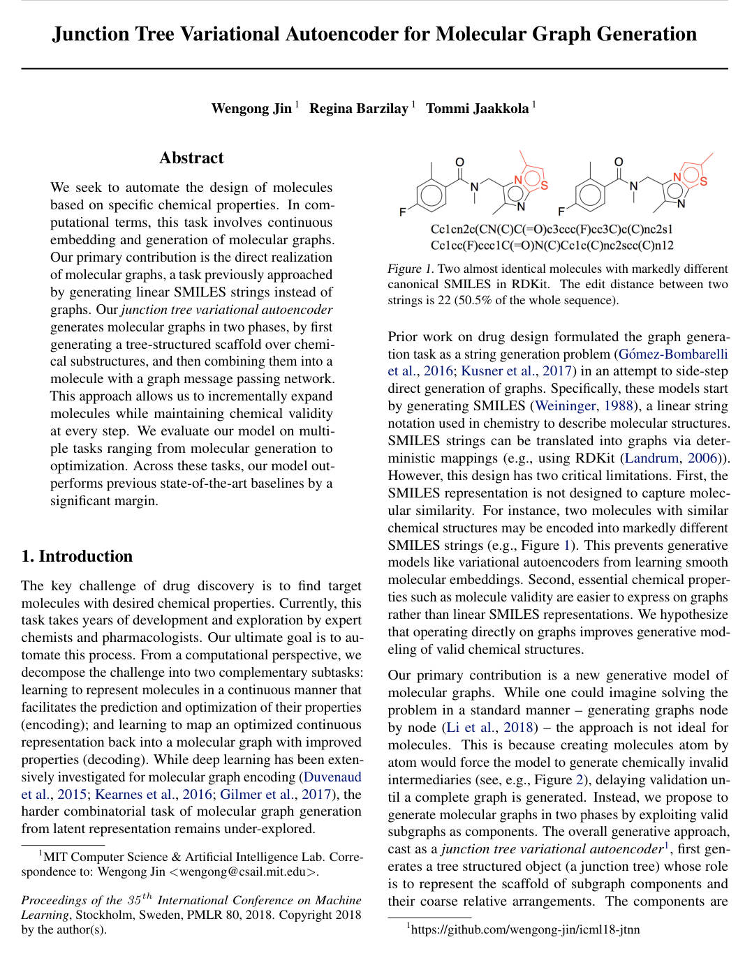
Cover for Junction Tree Variational Autoencoder for Molecular Graph Generation

Abstract

We seek to automate the design of molecules based on specific chemical properties. In computational terms, this task involves continuous embedding and generation of molecular graphs. Our primary contribution is the direct realization of molecular graphs, a task previously approached by generating linear SMILES strings instead of graphs. Our junction tree variational autoencoder generates molecular graphs in two phases, by first generating a tree-structured scaffold over chemical substructures, and then combining them into a molecule with a graph message passing network. This approach allows us to incrementally expand molecules while maintaining chemical validity at every step. We evaluate our model on multiple tasks ranging from molecular generation to optimization. Across these tasks, our model outperforms previous state-of-the-art baselines by a significant margin.

Topics

bipartite graphs optimization ranging variational autoencoders variational auto encoders variational methods

Keywords

Junction Tree Variational Autoencoder molecular graph generation molecule optimization molecular embeddings tree decomposition graph decoder graph encoder tree representation

1 Introduction
2 Junction Tree Variational Autoencoder
2.1 Junction Tree
2.2 Graph Encoder
2.3 Tree Encoder
2.4 Tree Decoder
2.5 Graph Decoder
3 Experiments
3.1 Molecule Reconstruction and Validity
3.2 Bayesian Optimization
3.3 Constrained Optimization
4 Related Work
5 Conclusion
References
A Tree Decomposition
B Stereochemistry
C Training Details
D More Experimental Results

Knowls

Knowl 1 — Two-Phase Molecular Graph Generation via Junction Tree Variational Autoencoder
model/method
The Junction Tree Variational Autoencoder (JT-VAE) is a generative framework for molecular graphs that decomposes generation into two phases: first generating a tree-structured scaffold of chemical substructure components (a junction tree), and then assembling these substructure components into a full molecular graph using a neural message passing network. This two-phase approach avoids chemically invalid intermediate structures encountered in atom-by-atom graph generation.

A molecule is represented by a molecular graph $G = (V, E)$ , where $V$ is the set of atoms and $E$ is the set of chemical bonds, together with an associated junction tree $T_G = (\mathcal{V}, \mathcal{E}, \mathcal{X})$ . Each node $C_i \in \mathcal{V}$ in the junction tree represents an induced subgraph cluster of $G$ (such as a ring or a single bond) drawn from a discrete cluster vocabulary $\mathcal{X}$ .

The latent space is factored into two complementary continuous representations:

$z = [z_T, z_G]$

where $z_T \in \mathbb{R}^{d_T}$ encodes the junction tree structure and cluster types without specifying exact atom-level attachments between neighboring clusters, and $z_G \in \mathbb{R}^{d_G}$ encodes the fine-grained atom-level connectivity of the full molecular graph. In the standard model configuration, $d_T = 28$ and $d_G = 28$ , yielding a combined latent dimension of $56$ .

The generative process proceeds in two matching stages:
1. Tree Decoding: A tree-structured decoder $p(T \mid z_T)$ generates a junction tree $\hat{T}$ top-down from $z_T$ .
2. Graph Decoding: A graph decoder $p(G \mid \hat{T}, z_G)$ predicts the fine-grained connectivity between adjacent clusters in $\hat{T}$ to realize the full molecular graph $\hat{G}$ .
Knowl 2 — Molecular Tree Decomposition Algorithm
algorithm
The molecular tree decomposition algorithm converts a molecular graph $G = (V, E)$ into a cycle-free junction tree $T_G = (\mathcal{V}, \mathcal{E}, \mathcal{X})$ over a vocabulary $\mathcal{X}$ of valid chemical substructures. Each cluster node $C_i = (V_i, E_i) \in \mathcal{V}$ is an induced subgraph of $G$ satisfying:
1. Union property: $\bigcup_i V_i = V$ and $\bigcup_i E_i = E$ .
2. Running intersection property: For all clusters $C_i, C_j, C_k$ , if $C_k$ is on the tree path between $C_i$ and $C_j$ , then $V_i \cap V_j \subseteq V_k$ .
To ensure that any two intersecting clusters share at most two atoms (which limits candidate assembly configurations during decoding), rings sharing more than two atoms are merged into bridged rings, and auxiliary clusters $V_0$ are added at intersections of three or more clusters to break cluster cycles.
Input: Molecular graph $G = (V, E)$
Output: Junction tree $T_G = (\mathcal{V}, \mathcal{E})$
1: $V_1 \leftarrow \text{set of bonds } (u, v) \in E \text{ not belonging to any rings}$
2: $V_2 \leftarrow \text{set of simple rings in } G$
3: for each pair of rings $r_1, r_2 \in V_2$ do
4: if $|r_1 \cap r_2| > 2$ then
5: Merge $r_1$ and $r_2$ into a single bridged ring cluster
6: end if
7: end for
8: $V_0 \leftarrow \text{atoms being the intersection of three or more clusters in } V_1 \cup V_2$
9: $\mathcal{V} \leftarrow V_0 \cup V_1 \cup V_2$
10: $\mathcal{E}_{\text{candidate}} \leftarrow \{(i, j) \in \mathcal{V} \times \mathcal{V} \mid |i \cap j| > 0\}$
11: for each edge $(i, j) \in \mathcal{E}_{\text{candidate}}$ do
12: if $i \in V_0$ or $j \in V_0$ then
13: $\text{weight}(i, j) \leftarrow \infty$
14: else
15: $\text{weight}(i, j) \leftarrow 1$
16: end if
17: end for
18: $T_G \leftarrow \text{Maximum spanning tree over cluster graph } (\mathcal{V}, \mathcal{E}_{\text{candidate}}, \text{weight})$
19: return $T_G$
On the ZINC database of ~250k drug molecules, this algorithm yields a vocabulary size of $|\mathcal{X}| = 780$ consisting solely of single bonds, simple rings, merged bridged rings, and individual atoms.
Knowl 3 — Loopy Message Passing Graph Encoder
model/method
The graph encoder maps a molecular graph $G = (V, E)$ into a continuous latent vector $z_G$ . Each vertex $v \in V$ is assigned an initial feature vector $x_v$ (encoding atom type, degree, formal charge, and chiral configuration), and each edge $(u, v) \in E$ is assigned a bond feature vector $x_{uv}$ (encoding bond type, ring membership, and cis-trans configuration).

Because molecular graphs contain cycles, message vectors $\nu_{uv}$ and $\nu_{vu}$ along edge $(u, v)$ are updated via loopy belief propagation over $T = 3$ iterations (initialized with $\nu_{uv}^{(0)} = 0$ ):

$\nu_{uv}^{(t)} = \tau\left(W_1^g x_u + W_2^g x_{uv} + W_3^g \sum_{w \in N(u) \setminus \{v\}} \nu_{wu}^{(t-1)}\right)$

where $N(u)$ is the set of neighbor atoms of $u$ , $\tau(\cdot)$ is the ReLU activation function, and $W_1^g, W_2^g, W_3^g$ are learned weight matrices.

After $T$ steps, latent vertex vectors $h_u$ are computed by aggregating inward messages:

$h_u = \tau\left(U_1^g x_u + \sum_{v \in N(u)} U_2^g \nu_{vu}^{(T)}\right)$

where $U_1^g, U_2^g$ are learned parameter matrices. The graph-level embedding is computed by mean pooling across all vertices:

$h_G = \frac{1}{|V|} \sum_{u \in V} h_u$

Two affine layers map $h_G$ to mean $\mu_G$ and log-variance $\log \sigma_G$ , from which $z_G \sim \mathcal{N}(\mu_G, \sigma_G)$ is sampled.
Knowl 4 — Tree Message Passing Encoder for Junction Trees
model/method
The tree encoder computes a continuous latent representation $z_T$ from a junction tree $T_G = (\mathcal{V}, \mathcal{E}, \mathcal{X})$ . Each node $C_i \in \mathcal{V}$ is represented by a learned cluster embedding $x_i$ corresponding to its label in vocabulary $\mathcal{X}$ .

Tree message passing propagates information in two phases over a rooted orientation of $T_G$ : a bottom-up phase from leaf nodes toward the root, and a top-down phase from the root to all leaves. The message $m_{ij}$ along tree edge $(C_i, C_j)$ is computed only when all inward precursor messages $\{m_{ki} \mid k \in N(i) \setminus \{j\}\}$ are available:

$s_{ij} = \sum_{k \in N(i) \setminus \{j\}} m_{ki}$

$z_{ij} = \sigma(W_z x_i + U_z s_{ij} + b_z)$

$r_{ki} = \sigma(W_r x_i + U_r m_{ki} + b_r)$

$\tilde{m}_{ij} = \tanh\left(W x_i + U \sum_{k \in N(i) \setminus \{j\}} r_{ki} \odot m_{ki}\right)$

$m_{ij} = (1 - z_{ij}) \odot s_{ij} + z_{ij} \odot \tilde{m}_{ij}$

where $\sigma(\cdot)$ is the sigmoid function, $\odot$ is element-wise multiplication, and $W_z, U_z, b_z, W_r, U_r, b_r, W, U$ are learned parameters of a tree Gated Recurrent Unit (GRU).

Each node representation $h_i$ is obtained by aggregating inward messages:

$h_i = \tau\left(W_o x_i + \sum_{k \in N(i)} U_o m_{ki}\right)$

where $\tau(\cdot)$ is ReLU. The tree-level latent representation is set directly to the root representation, $h_{T_G} = h_{\text{root}}$ , without average pooling to preserve the generative root orientation. Mean $\mu_T$ and log-variance $\log \sigma_T$ are computed via affine layers, and $z_T \sim \mathcal{N}(\mu_T, \sigma_T)$ .
Knowl 5 — Top-Down Depth-First Tree Decoder and Feasibility Filtering
algorithm
The tree decoder generates a junction tree $\hat{T}$ top-down in depth-first traversal order from the latent vector $z_T$ . At each step $t$ visiting node $i_t$ , the model makes a binary topological prediction $p_t$ on whether to expand a child node, and if expanding, predicts the label distribution $q_j$ over cluster vocabulary $\mathcal{X}$ .

Let $\tilde{\mathcal{E}}_t$ be the set of traversed directed edges up to step $t$ . Intermediate messages $h_{i_t, j_t}$ are computed with the tree GRU:

$h_{i_t, j_t} = \text{GRU}\left(x_{i_t}, \{h_{k, i_t}\}_{(k, i_t) \in \tilde{\mathcal{E}}_t, k \neq j_t}\right)$

Topological expansion probability $p_t$ is given by:

$p_t = \sigma\left(u_d \cdot \tau\left(W_1^d x_{i_t} + W_2^d z_T + W_3^d \sum_{(k, i_t) \in \tilde{\mathcal{E}}_t} h_{k, i_t}\right)\right)$

When a child $j$ is created from parent $i$ , its label distribution $q_j$ is:

$q_j = \text{softmax}\left(U_l \tau(W_1^l z_T + W_2^l h_{ij})\right)$

where $h_{ij} = 0$ if $j$ is the root node.

Training minimizes cross-entropy loss with teacher forcing:

$\mathcal{L}_c(T) = \sum_t \mathcal{L}_d(p_t, \hat{p}_t) + \sum_j \mathcal{L}_l(q_j, \hat{q}_j)$
Input: Latent representation $z_T$ , cluster vocabulary $\mathcal{X}$
Output: Decoded junction tree $\hat{T}$
1: Initialize: Tree $\hat{T} \leftarrow \emptyset$
2: function SampleTree(node $i$ , time step $t$ )
3: $\mathcal{X}_i \leftarrow \text{all cluster labels in } \mathcal{X} \text{ chemically compatible with node } i \text{ and its existing neighbors}$
4: Compute expansion probability $p_t$
5: Sample binary decision $d_t \in \{\text{expand}, \text{stop}\} \text{ from Bernoulli}(p_t)$
6: if $d_t = \text{expand}$ and $\mathcal{X}_i \neq \emptyset$ then
7: Create child node $j$ and add it to $\hat{T}$
8: Compute label distribution $q_j$ over $\mathcal{X}$
9: Renormalize $q_j$ over $\mathcal{X}_i$ by setting $q_j(c) = 0$ for all $c \notin \mathcal{X}_i$
10: Sample label for node $j$ from renormalized $q_j$
11: SampleTree( $j, t + 1$ )
12: end if
13: end function
Knowl 6 — Graph Decoder for Subgraph Assembly
model/method
The graph decoder reconstructs a molecular graph $\hat{G}$ from a predicted junction tree $\hat{T} = (\hat{\mathcal{V}}, \hat{\mathcal{E}})$ and latent vector $z_G$ . The task is formulated as structured prediction over candidate graphs $\mathcal{G}(\hat{T})$ :

$\hat{G} = \arg\max_{G' \in \mathcal{G}(\hat{T})} f_a(G')$

To ensure efficiency, subgraphs are assembled sequentially in the order nodes were decoded in $\hat{T}$ :
1. At each tree node $C_i$ , candidate subgraphs $G_i \in \mathcal{G}_i$ are enumerated by combining cluster $C_i$ with its tree neighbors $\{C_j \mid j \in N_{\hat{T}}(i)\}$ . Chemically invalid combinations are pruned and isomorphic subgraphs are merged.
2. In a candidate subgraph $G_i$ , let $\alpha_v = i$ if atom $v \in C_i$ and $\alpha_v = j$ if $v \in C_j \setminus C_i$ . Tree messages $\hat{m}_{\alpha_u, \alpha_v}$ computed by the tree encoder over $\hat{T}$ provide positional context for bond $(u, v)$ :
$\mu_{uv}^{(t)} = \tau\left(W_1^a x_u + W_2^a x_{uv} + W_3^a \tilde{\mu}_{uv}^{(t-1)}\right)$

$\tilde{\mu}_{uv}^{(t-1)} = \begin{cases} \sum_{w \in N(u) \setminus \{v\}} \mu_{wu}^{(t-1)} & \text{if } \alpha_u = \alpha_v \\ \hat{m}_{\alpha_u, \alpha_v} + \sum_{w \in N(u) \setminus \{v\}} \mu_{wu}^{(t-1)} & \text{if } \alpha_u \neq \alpha_v \end{cases}$
1. Vertex representations are aggregated into candidate subgraph representation $h_{G_i}$ , and scored as $f_a(G_i) = h_{G_i} \cdot z_G$ .
2. Graph decoder parameters are optimized by maximizing the log-likelihood of ground-truth subgraphs $G_i$ :
$\mathcal{L}_g(G) = \sum_i \left[ f_a(G_i) - \log \sum_{G'_i \in \mathcal{G}_i} \exp(f_a(G'_i)) \right]$

Because any two clusters share at most two atoms, candidate set size is small ( $|\mathcal{G}_i| \approx 4$ on average on ZINC), making the assembly complexity linear in the number of clusters.
Knowl 7 — Post-Hoc Stereochemistry Prediction and Total Training Loss
model/method
Because molecules possess three-dimensional stereochemical configurations (chiral centers and cis-trans isomerism) that are not easily modeled via formal grammars, the Junction Tree Variational Autoencoder separates stereochemical configuration prediction from 2D graph generation.

After generating the 2D molecular graph $m$ , all stereochemically valid 3D isomers $\mathcal{S}_m$ are enumerated using RDKit's EnumerateStereoisomers. For each candidate isomer $m' \in \mathcal{S}_m$ , the graph encoder computes an isomer embedding $h_{m'}$ , and scores the isomer using cosine similarity with the latent molecular representation $z_m$ :

$f^s(m') = \cos(h_{m'}, z_m)$

The final 3D structure is determined by selecting the highest-scoring isomer:

$\hat{m} = \arg\max_{m' \in \mathcal{S}_m} f^s(m')$

During training, the stereochemistry loss $\mathcal{L}_s$ maximizes the log-likelihood of the ground-truth stereoisomer $m$ :

$\mathcal{L}_s = f^s(m) - \log \sum_{m' \in \mathcal{S}_m} \exp(f^s(m'))$

The total molecular reconstruction loss $\mathcal{L}$ of JT-VAE is the sum of tree decoding loss $\mathcal{L}_c$ , graph assembly loss $\mathcal{L}_g$ , and stereochemistry loss $\mathcal{L}_s$ :

$\mathcal{L} = \mathcal{L}_c + \mathcal{L}_g + \mathcal{L}_s$

Knowl 8 — Molecular Reconstruction Accuracy and Prior Sampling Validity

data/table

Molecule reconstruction accuracy and sampling validity were evaluated on the 250k ZINC benchmark dataset with a 56-dimensional latent space. Reconstruction accuracy was measured via Monte Carlo sampling (each test molecule encoded 10 times and each latent code decoded 10 times; reported as the percentage of 100 decoded molecules identical to the input). Prior validity was evaluated by sampling 1,000 latent vectors from $\mathcal{N}(0, I)$ , decoding each 100 times, and checking chemical validity with RDKit.

Method	Reconstruction	Validity
CVAE (Gómez-Bombarelli et al., 2016)	44.6%	0.7%
GVAE (Kusner et al., 2017)	53.7%	7.2%
SD-VAE (Dai et al., 2018)	76.2%	43.5%
GraphVAE (Simonovsky Komodakis, 2018)	-	13.5%
Atom-by-Atom LSTM (Li et al., 2018)	-	89.2%
JT-VAE	76.7%	100.0%

JT-VAE achieved 76.7% reconstruction accuracy and 100.0% validity under prior sampling. In comparison, SMILES string-based models and node-by-node graph models frequently generate chemically invalid structures (achieving at most 43.5% and 89.2% validity, respectively). Furthermore, 5,000 molecules randomly sampled from the prior distribution of JT-VAE were verified to be 100% chemically valid, non-trivial, and completely distinct from the training set.

Knowl 9 — Bayesian Optimization on Learned Latent Space for Target Property Discovery

empirical result

Bayesian optimization (BO) was performed in the learned latent spaces of variational autoencoders to discover novel molecules maximizing penalized water-octanol partition coefficient:

$y(m) = \text{logP}(m) - \text{SA}(m) - \text{cycle}(m)$

where $\text{logP}(m)$ is the octanol-water partition coefficient, $\text{SA}(m)$ is the synthetic accessibility score, and $\text{cycle}(m)$ penalizes rings with more than 6 atoms. Scores were normalized to zero mean and unit variance using the training set.

A Sparse Gaussian Process (SGP) with 500 inducing points was trained on the latent encodings. Five iterations of batched BO (50 proposed latent points per batch using expected improvement) were conducted across 10 independent runs.

Top property scores of discovered molecules:

SGP property prediction performance (10-fold cross-validation on learned latent representations):

Method	Log-Likelihood (LL)	RMSE
CVAE	$-1.812 \pm 0.004$	$1.504 \pm 0.006$
GVAE	$-1.739 \pm 0.004$	$1.404 \pm 0.006$
SD-VAE	$-1.697 \pm 0.015$	$1.366 \pm 0.023$
JT-VAE	$\mathbf{-1.658 \pm 0.023}$	$\mathbf{1.290 \pm 0.026}$

JT-VAE found molecules with top property scores up to 5.30 (and found over 50 molecules scoring higher than SD-VAE's second-best score of 3.50) while providing latent representations that improved SGP log-likelihood and RMSE.

Knowl 10 — Constrained Molecule Optimization via Latent Gradient Ascent

empirical result

Constrained molecule optimization modifies an initial molecule $m$ to find a novel molecule $m'$ that maximizes penalized property $y(m') = \text{logP}(m') - \text{SA}(m')$ while satisfying a similarity constraint $\text{sim}(m, m') \ge \delta$ , where $\text{sim}(\cdot, \cdot)$ is the Tanimoto similarity over Morgan fingerprints (radius 2) and $\delta \in \{0.0, 0.2, 0.4, 0.6\}$ .

A property predictor $F$ (a feed-forward network with one 450-dimensional hidden layer and $\tanh$ activation) was jointly trained with JT-VAE to predict $y(m)$ from latent embeddings. Starting from mean encoding $z_m^{(0)} = \mu_m$ , $K = 80$ gradient ascent steps were executed:

$z_m^{(t)} = z_m^{(t-1)} + \alpha \frac{\partial F(z)}{\partial z}$

with step size $\alpha = 2.0$ . Molecules were decoded from the 80 latent trajectory points, and the highest-scoring candidate satisfying the similarity constraint and differing from $m$ was selected.

Evaluation on the 800 lowest-scoring molecules from the ZINC test set yielded:

$\delta$	Improvement $y(m') - y(m)$	Similarity $\text{sim}(m, m')$	Success Rate
0.0	$1.91 \pm 2.04$	$0.28 \pm 0.15$	97.5%
0.2	$1.68 \pm 1.85$	$0.33 \pm 0.13$	97.1%
0.4	$0.84 \pm 1.45$	$0.51 \pm 0.10$	83.6%
0.6	$0.21 \pm 0.71$	$0.69 \pm 0.06$	46.4%

Under moderate structural similarity constraints ( $\delta = 0.4$ ), the model successfully discovered improved valid molecules in 83.6% of cases with an average property improvement of $0.84$ .

Coverage note — No substantial contributed material was omitted.

References

1.Aharoni, R. and Goldberg, Y. Towards string-to-tree neural machine translation. arXiv preprint arXiv:1704.04743, 2017.
2.Alvarez-Melis, D. and Jaakkola, T. S. Tree-structured decoding with doubly-recurrent neural networks. 2016.
3.Besnard, J., Ruda, G. F., Setola, V., Abecassis, K., Rodriguiz, R. M., Huang, X.-P., Norval, S., Sassano, M. F., Shin, A. I., Webster, L. A., et al. Automated design of ligands to polypharmacological profiles. Nature, 492(7428): 215–220, 2012.
4.Bruna, J., Zaremba, W., Szlam, A., and LeCun, Y. Spectral networks and locally connected networks on graphs. arXiv preprint arXiv:1312.6203, 2013.
5.Chung, J., Gulcehre, C., Cho, K., and Bengio, Y. Empirical evaluation of gated recurrent neural networks on sequence modeling. arXiv preprint arXiv:1412.3555, 2014.
6.Clayden, J., Greeves, N., Warren, S., and Wothers, P. Organic Chemistry. Oxford University Press, 2001.
7.Dai, H., Dai, B., and Song, L. Discriminative embeddings of latent variable models for structured data. In International Conference on Machine Learning, pp. 2702–2711, 2016.
8.Dai, H., Tian, Y., Dai, B., Skiena, S., and Song, L. Syntax-directed variational autoencoder for structured data. International Conference on Learning Representations, 2018. URL https://openreview.net/forum?id=SyqShMZRb.
9.Dong, L. and Lapata, M. Language to logical form with neural attention. arXiv preprint arXiv:1601.01280, 2016.
10.Duvenaud, D. K., Maclaurin, D., Iparraguirre, J., Bombarell, R., Hirzel, T., Aspuru-Guzik, A., and Adams, R. P. Convolutional networks on graphs for learning molecular fingerprints. In Advances in neural information processing systems, pp. 2224–2232, 2015.
11.Dyer, C., Kuncoro, A., Ballesteros, M., and Smith, N. A. Recurrent neural network grammars. arXiv preprint arXiv:1602.07776, 2016.
12.Gilmer, J., Schoenholz, S. S., Riley, P. F., Vinyals, O., and Dahl, G. E. Neural message passing for quantum chemistry. arXiv preprint arXiv:1704.01212, 2017.
13.Gómez-Bombarelli, R., Wei, J. N., Duvenaud, D., Hernández-Lobato, J. M., Sánchez-Lengeling, B., Sheberla, D., Aguilera-Iparraguirre, J., Hirzel, T. D., Adams, R. P., and Aspuru-Guzik, A. Automatic chemical design using a data-driven continuous representation of molecules. ACS Central Science, 2016. doi: 10.1021/acscentsci.7b00572.
14.Gori, M., Monfardini, G., and Scarselli, F. A new model for learning in graph domains. In Neural Networks, 2005. IJCNN'05. Proceedings. 2005 IEEE International Joint Conference on, volume 2, pp. 729–734. IEEE, 2005.
15.Guimaraes, G. L., Sanchez-Lengeling, B., Farias, P. L. C., and Aspuru-Guzik, A. Objective-reinforced generative adversarial networks (organ) for sequence generation models. arXiv preprint arXiv:1705.10843, 2017.
16.Henaff, M., Bruna, J., and LeCun, Y. Deep convolutional networks on graph-structured data. arXiv preprint arXiv:1506.05163, 2015.
17.Janz, D., van der Westhuizen, J., and Hernández-Lobato, J. M. Actively learning what makes a discrete sequence valid. arXiv preprint arXiv:1708.04465, 2017.
18.Jin, W., Coley, C., Barzilay, R., and Jaakkola, T. Predicting organic reaction outcomes with weisfeiler-lehman network. In Advances in Neural Information Processing Systems, pp. 2604–2613, 2017.
19.Kearnes, S., McCloskey, K., Berndl, M., Pande, V., and Riley, P. Molecular graph convolutions: moving beyond fingerprints. Journal of computer-aided molecular design, 30(8):595–608, 2016.
20.Kingma, D. P. and Welling, M. Auto-encoding variational bayes. arXiv preprint arXiv:1312.6114, 2013.
21.Kiperwasser, E. and Goldberg, Y. Easy-first dependency parsing with hierarchical tree lstms. arXiv preprint arXiv:1603.00375, 2016.
22.Kipf, T. N. and Welling, M. Semi-supervised classification with graph convolutional networks. arXiv preprint arXiv:1609.02907, 2016.
23.Kusner, M. J., Paige, B., and Hernández-Lobato, J. M. Grammar variational autoencoder. arXiv preprint arXiv:1703.01925, 2017.
24.Landrum, G. Rdkit: Open-source cheminformatics. Online). http://www. rdkit. org. Accessed, 3(04):2012, 2006.
25.Lei, T., Jin, W., Barzilay, R., and Jaakkola, T. Deriving neural architectures from sequence and graph kernels. arXiv preprint arXiv:1705.09037, 2017.
26.Li, Y., Tarlow, D., Brockschmidt, M., and Zemel, R. Gated graph sequence neural networks. arXiv preprint arXiv:1511.05493, 2015.
27.Li, Y., Vinyals, O., Dyer, C., Pascanu, R., and Battaglia, P. Learning deep generative models of graphs. arXiv preprint arXiv:1803.03324, 2018.
28.Monti, F., Boscaini, D., Masci, J., Rodolà, E., Svoboda, J., and Bronstein, M. M. Geometric deep learning on graphs and manifolds using mixture model cnns. arXiv preprint arXiv:1611.08402, 2016.
29.Mueller, J., Gifford, D., and Jaakkola, T. Sequence to better sequence: continuous revision of combinatorial structures. In International Conference on Machine Learning, pp. 2536–2544, 2017.
30.Niepert, M., Ahmed, M., and Kutzkov, K. Learning convolutional neural networks for graphs. In International Conference on Machine Learning, pp. 2014–2023, 2016.
31.Parisotto, E., Mohamed, A.-r., Singh, R., Li, L., Zhou, D., and Kohli, P. Neuro-symbolic program synthesis. arXiv preprint arXiv:1611.01855, 2016.
32.Rarey, M. and Dixon, J. S. Feature trees: a new molecular similarity measure based on tree matching. Journal of computer-aided molecular design, 12(5):471–490, 1998.
33.Rogers, D. and Hahn, M. Extended-connectivity fingerprints. Journal of chemical information and modeling, 50(5):742–754, 2010.
34.Scarselli, F., Gori, M., Tsoi, A. C., Hagenbuchner, M., and Monfardini, G. The graph neural network model. IEEE Transactions on Neural Networks, 20(1):61–80, 2009.
35.Schütt, K., Kindermans, P.-J., Felix, H. E. S., Chmiela, S., Tkatchenko, A., and Müller, K.-R. Schnet: A continuous-filter convolutional neural network for modeling quantum interactions. In Advances in Neural Information Processing Systems, pp. 992–1002, 2017.
36.Segler, M. H., Kogej, T., Tyrchan, C., and Waller, M. P. Generating focussed molecule libraries for drug discovery with recurrent neural networks. arXiv preprint arXiv:1701.01329, 2017.
37.Simonovsky, M. and Komodakis, N. Graphvae: Towards generation of small graphs using variational autoencoders. arXiv preprint arXiv:1802.03480, 2018.
38.Socher, R., Perelygin, A., Wu, J., Chuang, J., Manning, C. D., Ng, A., and Potts, C. Recursive deep models for semantic compositionality over a sentiment treebank. In Proceedings of the 2013 conference on empirical methods in natural language processing, pp. 1631–1642, 2013.
39.Sterling, T. and Irwin, J. J. Zinc 15–ligand discovery for everyone. J. Chem. Inf. Model, 55(11):2324–2337, 2015.
40.Tai, K. S., Socher, R., and Manning, C. D. Improved semantic representations from tree-structured long short-term memory networks. arXiv preprint arXiv:1503.00075, 2015.
41.Vinyals, O., Kaiser, Ł., Koo, T., Petrov, S., Sutskever, I., and Hinton, G. Grammar as a foreign language. In Advances in Neural Information Processing Systems, pp. 2773–2781, 2015.
42.Weininger, D. Smiles, a chemical language and information system. 1. introduction to methodology and encoding rules. Journal of chemical information and computer sciences, 28(1):31–36, 1988.
43.Zhu, X., Sobihani, P., and Guo, H. Long short-term memory over recursive structures. In International Conference on Machine Learning, pp. 1604–1612, 2015.

Citation

MLA

Jin, W., et al. “Junction Tree Variational Autoencoder for Molecular Graph Generation”. arXiv, 2018, http://arxiv.org/abs/1802.04364v4.

APA

Jin, W., Barzilay, R., & Jaakkola, T. (2018). Junction Tree Variational Autoencoder for Molecular Graph Generation. arXiv. http://arxiv.org/abs/1802.04364v4

Chicago

Jin, W., R. Barzilay, and T. Jaakkola. 2018. “Junction Tree Variational Autoencoder for Molecular Graph Generation”. arXiv. http://arxiv.org/abs/1802.04364v4.

Harvard

Jin, W., Barzilay, R. and Jaakkola, T. (2018) “Junction Tree Variational Autoencoder for Molecular Graph Generation”, arXiv [Preprint]. Available at: http://arxiv.org/abs/1802.04364v4.

Vancouver

1. Jin W, Barzilay R, Jaakkola T (2018) Junction Tree Variational Autoencoder for Molecular Graph Generation. arXiv

BibTeX

@article{jin2018junction,
  title = {Junction Tree Variational Autoencoder for Molecular Graph Generation},
  author = {Jin, Wengong and Barzilay, Regina and Jaakkola, Tommi},
  year = {2018},
  journal = {arXiv},
  url = {http://arxiv.org/abs/1802.04364v4},
  eprint = {1802.04364}
}

Metadata:arXiv

Source Code

This paper has an official code repository available. Click below to access the source code.

View Repository

Access the Paper

This paper is available from its original source. Click below to access the PDF.

Open PDF

License: https://creativecommons.org/licenses/by/4.0/

Method	1st	2nd	3rd
CVAE	1.98	1.42	1.19
GVAE	2.94	2.89	2.80
SD-VAE	4.04	3.50	2.96
JT-VAE	5.30	4.93	4.49

Junction Tree Variational Autoencoder for Molecular Graph Generation

Abstract

Topics

Keywords

Table of Contents

Knowls

Knowl 1 — Two-Phase Molecular Graph Generation via Junction Tree Variational Autoencoder

Knowl 2 — Molecular Tree Decomposition Algorithm

Knowl 3 — Loopy Message Passing Graph Encoder

Knowl 4 — Tree Message Passing Encoder for Junction Trees

Knowl 5 — Top-Down Depth-First Tree Decoder and Feasibility Filtering

Knowl 6 — Graph Decoder for Subgraph Assembly

Knowl 7 — Post-Hoc Stereochemistry Prediction and Total Training Loss