
Flow Reasoning Models: Turning Flows Into Efficient Recurrent Reasoners
Alec Helbling$^{1,3,4,}$ Andrey Bryutkin$^{2,3,4,}$ Mauro Martino$^{3,4}$
Duen Horng (Polo) Chau$^{1}$ Nima Dehmamy$^{3,4}$ Hendrik Strobelt$^{3,4}$
$^{1}$Georgia Tech $^{2}$MIT $^{3}$MIT-IBM Computing Research Lab $^{4}$IBM Research
$^{*}$ Co-first author. Correspondence to Alec Helbling: [email protected]
Abstract
Structured reasoning requires making and revising interdependent decisions to reach a globally consistent solution. Existing architectures struggle with this: autoregressive models commit sequentially and cannot revise earlier decisions, while masked diffusion models often require careful decoding schemes to coordinate interdependent predictions. We introduce Flow Reasoning Models (FRMs), a novel framework for structured reasoning that adapts continuous flows over discrete structured outputs with a simple recurrent refinement mechanism. By self-conditioning a flow model on its own past outputs, we turn one-shot denoising into iterative solution refinement. This lets FRMs make and revise decisions in parallel, efficiently coordinating interdependent choices across solutions. Yet conventional self-conditioning becomes unreliable at greater recurrent depth due to exposure bias between one-step training predictions and recursively generated inference states. We address this mismatch with Fixed-Point Forcing (FPF), which trains FRMs on states produced by their own inference dynamics while preserving the standard flow-matching objective. FRMs achieve solve rates of 99.5%, 100.0%, and 99.9% on Sudoku-Extreme, Zebra, and Maze-Unique, respectively. On Sudoku-Extreme, FRMs achieve higher peak accuracy than the evaluated masked-diffusion and specialized reasoning baselines while remaining highly compute-efficient, matching the next-best method's 98.7% peak solve rate with $44\times$ fewer inference FLOPs.
Executive Summary: Flow Reasoning Models (FRMs) address the challenge of structured reasoning tasks, such as solving tightly constrained puzzles, where models must coordinate many interdependent decisions into one consistent output. Autoregressive models commit to choices in sequence without revision, while masked diffusion approaches often produce inconsistencies during parallel updates and require extra mechanisms to correct errors. These limitations matter because many real-world planning, scheduling, and deduction problems share the same need for global consistency under tight constraints.
The work set out to show that continuous flow models over discrete data can be turned into recurrent reasoners that iteratively refine candidate solutions. The authors introduced self-conditioning to create recurrence and a new training procedure called Fixed-Point Forcing (FPF) to close the gap between training and inference states.
They evaluated the approach on three benchmarks—Sudoku-Extreme, Zebra, and Maze-Unique—using exact solve rate as the primary metric and total inference FLOPs to measure efficiency. Experiments compared FRMs against vanilla discrete flows, masked diffusion models, and specialized recurrent reasoners, with training performed from scratch on each dataset and results aggregated over multiple seeds.
FRMs reached peak solve rates of 99.5 percent on Sudoku-Extreme, 100 percent on Zebra, and 99.9 percent on Maze-Unique. On Sudoku-Extreme they matched the next-best published peak while using roughly 44 times fewer inference FLOPs. Self-conditioning alone raised performance over plain flows but plateaued; FPF removed the plateau, allowed deeper refinement to keep improving accuracy, and made convergence a near-perfect predictor of correctness. Vanilla flows showed little gain from extra compute, and conventional self-conditioning produced confidently wrong fixed points on harder instances.
These results indicate that recurrent reasoning can emerge from a standard flow-matching objective without custom latent-state architectures, delivering both higher accuracy and substantially better compute efficiency on constraint-satisfaction and path-finding tasks. The method preserves the canonical training objective and requires no backpropagation through time.
The authors recommend scaling the approach to larger models and less structured domains. Further work is needed to test robustness on tasks without unique solutions and to confirm whether the observed efficiency gains hold at language-model scale. The main limitations are that results rest on three specific benchmarks and that several baseline reproductions on Zebra could not be matched to published numbers, leaving some comparisons incomplete.
1. Introduction
Section Summary: The introduction highlights how structured reasoning tasks demand consistent coordination across many interdependent decisions, yet autoregressive and masked diffusion models often fail here due to irreversible commitments or conditionally independent updates that lead to inconsistencies. The authors address this by introducing Flow Reasoning Models, which adapt continuous flow models over discrete outputs with self-conditioning to enable iterative, recurrent refinement of candidate solutions. They further propose Fixed-Point Forcing to correct exposure bias during training, allowing the models to converge reliably toward correct answers as stable attractors and achieve strong accuracy with far lower computational cost than prior approaches on tasks such as Sudoku.
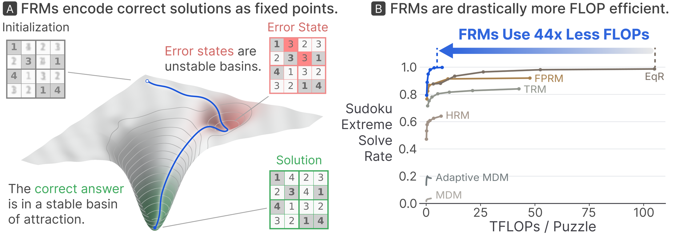
A central challenge in structured reasoning is coordinating many mutually constraining decisions into a single consistent solution. Autoregressive models often struggle with such tasks because they commit to tokens in a fixed order, without the ability to later revise them as their global consequences become clear. Masked diffusion models ([1]) offer a flexible generation order and predict multiple tokens in parallel, but tokens updated within the same step are conditionally independent given the current state and cannot condition on one another's realized values, making aggressive parallel updates prone to inconsistencies ([2]). Tightly constrained problems therefore require many conservative updates, and correcting earlier errors requires additional mechanisms such as remasking ([3]).
Continuous flow models over discrete data offer a promising alternative, modeling all tokens and their interdependencies simultaneously. Recent work has demonstrated that continuous flow models can effectively perform unconditional generation of natural language ([4, 5]), but their ability to perform structured reasoning remains largely unexplored. Indeed, in our own experiments, a naive application of such continuous flows to structured reasoning tasks like Sudoku solves only approximately $13%$ on the Sudoku-Extreme benchmark ([6]).
We introduce Flow Reasoning Models (FRMs), which turn continuous flows over discrete outputs into recurrent reasoning models that iteratively refine candidate solutions. Self-conditioning has previously been used to improve unconditional generation ([7, 5]). We observe that it can be particularly useful for decomposing complex reasoning into successive refinement steps: FRMs feed each prediction back into the flow as the state to be refined at the next step. This yields an interpretable recurrent state that can be directly decoded into the model's current candidate solution. It also provides a training-efficient form of recurrence that requires no backpropagation through time and retains the canonical flow-matching objective. Adding self-conditioning alone significantly improves performance, raising the solve rate on Sudoku-Extreme from roughly $13%$ to $33%$, but still leaving most problems unsolved.
This limitation becomes clearer through a dynamical-systems interpretation of FRMs: recurrent refinement performs learned fixed-point iteration over candidate solutions. Under this view, correct solutions should form stable, error-correcting attractors, while incorrect states should remain transient. Conventional self-conditioning fails to produce these dynamics on challenging problems, instead converging to confidently incorrect fixed points. We trace this failure to exposure bias between the one-step conditioning states used during training and the recursively generated states encountered during inference ([8, 9]). We introduce Fixed-Point Forcing (FPF), which trains on rollout-derived conditioning states so that the model learns to correct states produced by its own dynamics. Our results support this attractor picture: under FPF, recurrent refinement moves predictions toward the ground truth, correct solutions converge while incorrect states remain dynamically active, and convergence becomes strongly predictive of correctness.
Our core contributions are as follows:
- Flow Reasoning Models (FRMs), a novel generative modeling framework that turns continuous flows over discrete structured outputs into recurrent models for reasoning. Their predictions form an interpretable, directly decodable reasoning state while the models retain the canonical flow-matching objective and require no backpropagation through time.
- Fixed-Point Forcing (FPF), a novel training method for recurrent self-conditioned flow models. We discover that exposure bias can cause these models to converge to spurious fixed points. FPF mitigates this mismatch by training on rollout-derived conditioning states, making additional recurrent depth productive and convergence predictive of correctness.
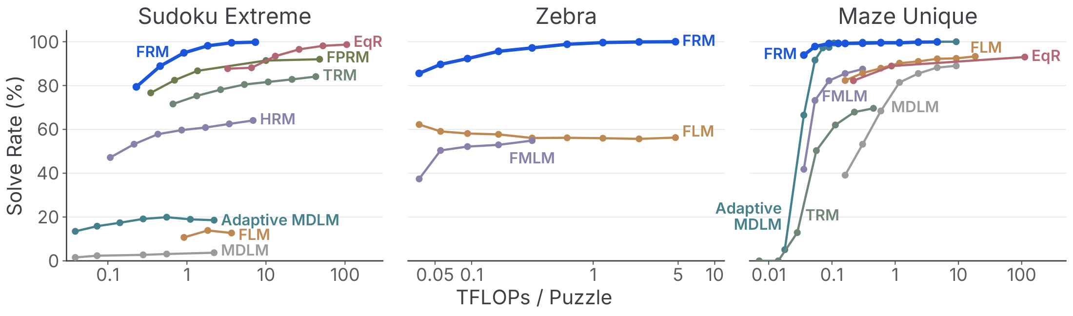
- State-of-the-art accuracy and efficiency across structured reasoning tasks. Across Sudoku-Extreme, Maze, and Zebra, FRMs achieve state-of-the-art solve rates and compare favorably with masked diffusion models and specialized small reasoning models in accuracy and inference efficiency. On Sudoku-Extreme, FRMs reach a peak solve rate of $99.5%$ and match EqR's peak $98.7%$ solve rate ([10]) with $44\times$ fewer inference FLOPs (Figure 1).

2. Flow Reasoning Models
Section Summary: Flow reasoning models treat problem solving as a conditional generation task in which a neural network gradually transforms random noise into a structured discrete solution, such as a completed Sudoku grid, while keeping the problem description fixed. The core mechanism is a discrete flow-matching process that predicts clean tokens at each step, trained with a standard cross-entropy loss. Adding self-conditioning turns the denoiser into a recurrent system that repeatedly feeds its own prior predictions back as extra input, allowing the model to refine earlier decisions, correct inconsistencies, and perform multiple reasoning updates at any point along the flow trajectory.
2.1 Discrete Flows for Conditional Reasoning
We formulate reasoning as conditional generation over data pairs $(c, y)\sim p_{\mathrm{data}}$. Here $c$ denotes the observed problem specification, for example, the given clues in Sudoku or the maze layout, and $y=(y_1, \ldots, y_L)$ denotes its discrete solution over vocabulary $\mathcal V$. Only the solution is noised and generated: $c$ is supplied as a separate conditioning input and held fixed throughout training and inference. Following work that models discrete data through continuous or simplex-valued representations ([11, 12, 7, 13]), we encode $y$ as a one-hot endpoint $x_1\in{0, 1}^{L\times|\mathcal V|}$ and decode predictions by positionwise argmax.
Flow matching connects Gaussian noise $\varepsilon\sim\mathcal N(0, I)$ to this endpoint along a probability path ([14, 15]). We use the linear interpolant
$ x_t=(1-t)\varepsilon+t x_1, \qquad t\in[0, 1].\tag{1} $
We adopt the categorical clean-prediction parameterization of Flow Language Models ([4]): a denoiser $D_\theta^t(x_t\mid c)$ predicts a categorical distribution over the clean token at each position. The corresponding clean endpoint prediction determines the probability-flow velocity:
$ v_\theta^t(x_t\mid c)=\bigl(D_\theta^t(x_t\mid c)-x_t\bigr)/(1-t).\tag{2} $
The same output is therefore both a directly decodable candidate solution and the quantity used to advance the flow. We train it with tokenwise cross-entropy,
$ \mathcal L_{\mathrm{CE}}(\theta)= \mathbb{E}{t, c, y, \varepsilon}!\left[-\sum{i=1}^{L} \log D_\theta^t(x_t\mid c)_{i, y_i}\right].\tag{3} $
This standard discrete-flow model is our FLM baseline. On its own it leaves a substantial gap on structured reasoning; FRMs add a recurrent axis while retaining this path and objective.
2.2 Self-Conditioning as Recurrent Reasoning
Self-conditioning.
Self-conditioning augments a denoiser with its own previous output as an additional input ([7]). We write the resulting model as $D_\theta^t(x_t\mid c, s)$, where $s$ carries a previous clean-solution prediction and $s=\varnothing$ denotes a zero-valued null carry. Conventional training uses two passes: a null-carry pass produces the detached prediction $\widetilde{s}=\operatorname{stopgrad}[D_\theta^t(x_t\mid c, \varnothing)]$, and the supervised pass receives either $\widetilde{s}$ or the null carry. The probability path and endpoint loss in Equation 3 remain unchanged, and gradients do not pass through $\widetilde{s}$.
Self-conditioning creates recurrence.
At inference, FRMs repeatedly feed the latest clean prediction back through $s$. This feedback lets later evaluations preserve useful decisions, revise inconsistent ones, and correct earlier mistakes. It also creates a discrete reasoning depth $k$, separate from continuous flow time $t$. Holding $(x_t, t)$ fixed, recurrent refinement is
$ s_t^{(0)}=\varnothing, \qquad s_t^{(k+1)}=D_\theta^t(x_t\mid c, s_t^{(k)}),\tag{4} $
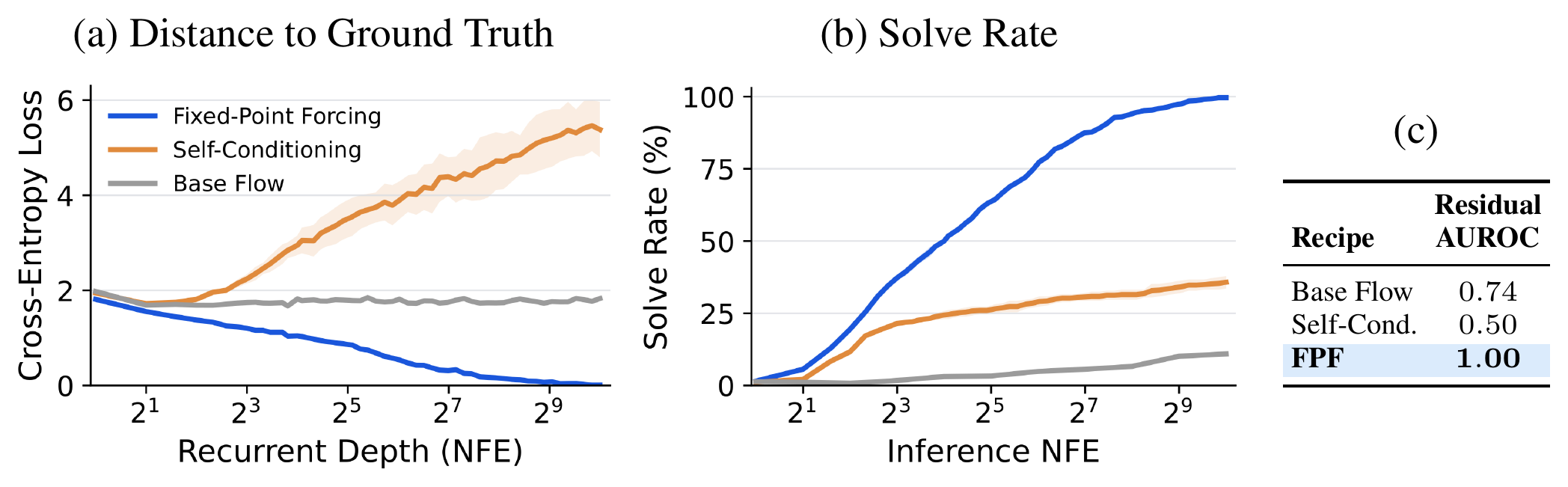
so each carry directly estimates the same clean solution. This gives every update direct supervision, allowing detached training without backpropagation through time. A sampler can alternate between advancing the flow state $x_t$ and applying additional recurrent updates at the current flow time. Although self-conditioning substantially improves refinement, its gains saturate with depth on Sudoku-Extreme (Figure 6 b), motivating the fixed-point analysis and training method developed next.

3. Fixed-Point Forcing Promotes Correct Solutions as Stable Attractors
Section Summary: The section explains that these models refine candidate answers through repeated internal feedback, but conventional training creates a mismatch: the system learns from single quick guesses rather than from its own ongoing chain of predictions. As a result, errors can get reinforced and settle into stable but wrong answers instead of being corrected. Fixed-point forcing addresses this by deliberately training the model on the kinds of intermediate states its own multi-step process actually produces, so that correct solutions become the natural resting points the system converges to.
The recurrence in Equation 4 defines a dynamical system over candidate solutions. Fixing $(x_t, c, t)$, repeated application of $D_\theta^t$ performs fixed-point iteration over the self-conditioning state. During an FPF rollout, however, the flow state, time, and carry evolve jointly, so this fixed-point iteration is a held-state view rather than a literal description of how the FPF carry is constructed. Flow time moves through a family of denoising problems, while reasoning depth iterates the corresponding denoiser toward a stable prediction. For a problem $c$ with goal $y^\star$, the desired held-state behavior is
$ s_t^{(k)}\longrightarrow s_t^\star, \qquad D_\theta^t(x_t\mid c, s_t^\star)=s_t^\star, \qquad \operatorname{decode}(s_t^\star)=y^\star.\tag{5} $
A useful solution should be attracting: imperfect nearby states should move toward it under additional reasoning depth. Stable states that decode to incorrect solutions are instead spurious fixed points. This perspective supplies a common language for the rest of the paper: training determines the recurrent state distribution, inference probes the resulting closed-loop dynamics, and useful test-time computation requires those dynamics to correct rather than stabilize errors.
3.1 Exposure Bias in the Recurrent State
Conventional self-conditioning trains with a detached one-pass carry produced from the ground-truth-derived interpolant $x_t=(1-t)\varepsilon+t y$, with $\widetilde{s}=\operatorname{stopgrad}[D_\theta^t(x_t\mid c, \varnothing)]$ (Figure 4, left). Recurrent inference instead feeds predictions back repeatedly, so the carry at depth $k$ is generated by the model's own closed-loop dynamics rather than by one pass from a ground-truth-derived state. Training and inference therefore induce different carry distributions,
$ p_{\mathrm{train}}(s\mid x_t, c, t) \neq p_{\mathrm{infer}}^{(k)}(s\mid \widehat{x}_t, c, t),\tag{6} $
and the mismatch grows with depth.
This mismatch has two coupled effects. First, the denoiser is not calibrated for its own recurrent states: an incorrect but overconfident prediction can be fed back as reliable evidence, amplify its error, and settle at a spurious fixed point. Second, one-pass training rarely presents the subtle, low-residual errors that remain after several refinement steps, so the model is not trained to correct precisely the states encountered near convergence. On challenging problems, recurrence can therefore stabilize and sharpen an incorrect solution, increasing gold-target cross-entropy with depth (Figure 6).
3.2 Fixed-Point Forcing
Fixed-Point Forcing (FPF) replaces the one-pass carry used in conventional self-conditioning with a detached carry produced by the model's own multi-step inference dynamics. It thereby trains each recurrent update on the kinds of states produced by earlier updates, directly targeting the train–inference mismatch in Equation 6.
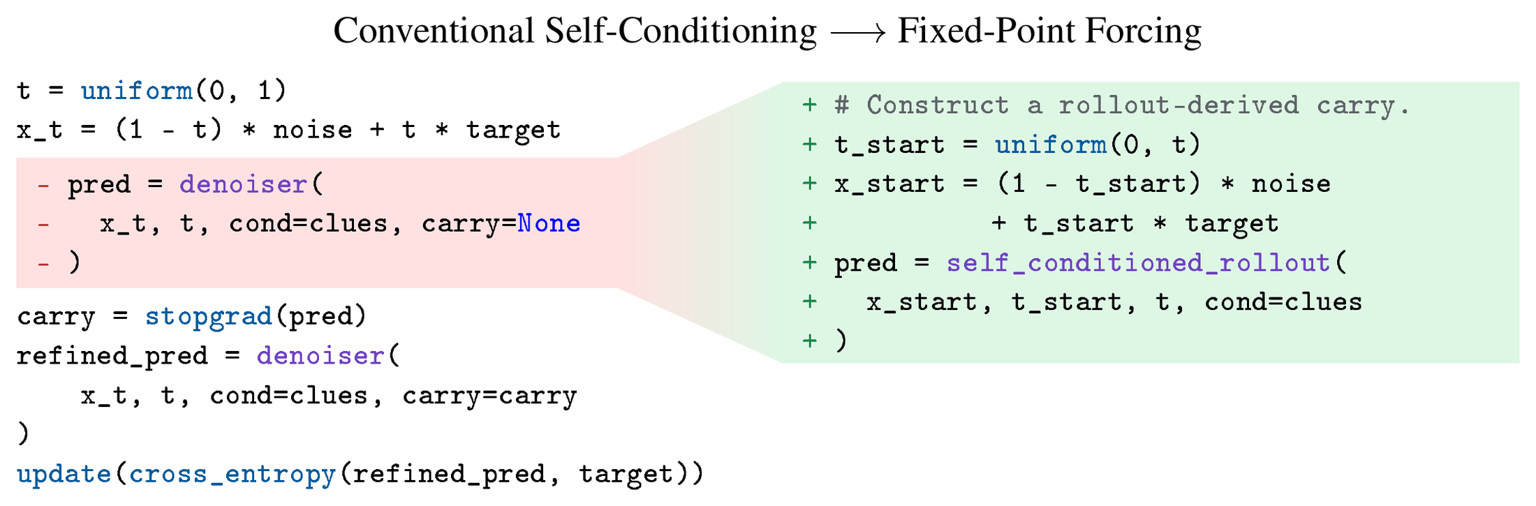
The conceptual difference is illustrated in Figure 3, and the corresponding training-code change is shown in Figure 4. We construct the FPF conditioning state by sampling a supervision time $t$ and a rollout start $t_{\mathrm{start}}\sim\mathcal{U}(0, t)$, then run the inference-time self-conditioned integrator from $t_{\mathrm{start}}$ to $t$. Its final prediction $s_{\mathrm{FPF}}$ is detached and supplied to the loss-bearing prediction $D_\theta^t(x_t\mid c, \operatorname{stopgrad}(s_{\mathrm{FPF}}))$; gradients do not pass through the rollout.
Crucially, this construction preserves the canonical flow-matching path exactly. As in conventional self-conditioning, the loss-bearing input remains $x_t=(1-t)\varepsilon+t y$, the target remains $y$, and the endpoint cross-entropy is unchanged; the rollout prediction enters only through the self-conditioning channel. FPF therefore changes the distribution of what the denoiser conditions on, not the state at which the flow objective is supervised. Training on rollout-derived carries reduces the carry-side exposure bias and the resulting overconfidence and miscalibration, while deeper rollout states expose the model to the smaller, subtler residual errors that remain near convergence and train the local corrections needed around a fixed point.
4. Experiments
Section Summary: Flow Reasoning Models were tested on three challenging structured reasoning benchmarks—Sudoku-Extreme, Zebra, and Maze-Unique—where they reached near-perfect exact solve rates of 99.5–100 percent while using far less computation than prior methods. The models outperformed both diffusion-based language models and specialized recurrent reasoners on accuracy-versus-compute curves, largely because self-conditioning and a new Fixed-Point Forcing training procedure let them repeatedly revise and improve partial solutions over multiple steps. In contrast, simpler flow baselines plateaued quickly, and conventional self-conditioning alone often produced confident but incorrect answers when run for many iterations.
We evaluate Flow Reasoning Models (FRMs) on Sudoku-Extreme, Zebra, and Maze-Unique, three structured-prediction benchmarks with different constraints and output structures. Our primary metric is exact solve rate. We compare inference efficiency using total FLOPs per instance and report the number of function evaluations (NFE) to describe how each method allocates iterative computation. Full protocols, baseline provenance, compute accounting, sweeps, and dynamics diagnostics appear in Appendix A.1–Appendix C.
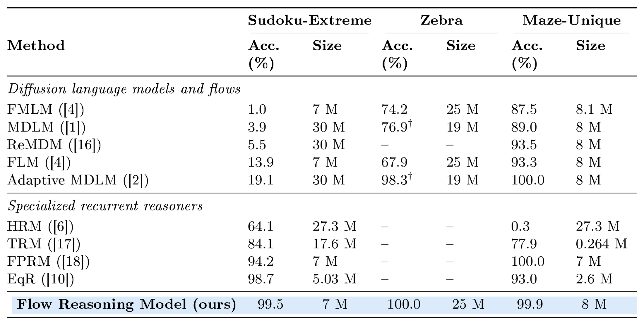
::: {caption="Table 1: Peak exact-solve accuracy and model size across structured reasoning tasks. Parameter counts correspond to the evaluated configuration and are rounded to the nearest reported model-size convention. Dashes indicate an unreported result or unavailable configuration-matched count. †Published Zebra result not reproduced in our evaluation pipeline; see Appendix A.3."}
:::
4.1 Accuracy and Efficiency Across Structured Reasoning Tasks
Flow Reasoning Models achieve near-perfect exact solving across distinct reasoning domains.
FRMs reach peak solve rates of $99.5%$ on Sudoku-Extreme, $100.0%$ on Zebra, and $99.9%$ on Maze-Unique (Table 1). These benchmarks require constraint satisfaction, relational deduction, and path finding, respectively, and differ substantially in sequence length, vocabulary, and output structure. Near-perfect performance across all three therefore shows that recurrent flow refinement is not tied to a particular task representation or constraint structure.
FRMs establish a stronger accuracy–compute frontier than diffusion language models and specialized recurrent reasoners.
FRM leads the measured accuracy–compute frontier on all three tasks (Figure 5). On Sudoku-Extreme, it attains the highest solve rate and reaches EqR's $98.7%$ peak with an estimated $44\times$ fewer inference FLOPs. FRM likewise dominates the measured Maze-Unique frontier, although its $99.9%$ peak is slightly below the best observed $100.0%$, and reaches $100.0%$ on Zebra, exceeding both reported peaks and the measured baselines. Zebra contains fewer curves because we could not reproduce several published MDM models reliably enough for FLOP profiling; their daggered, table-only accuracies and full provenance appear in Table 1 and Appendix A.3.
4.2 Self-Conditioning Enables Recurrent Refinement
Vanilla discrete flows achieve limited peak performance and do not scale with inference compute.
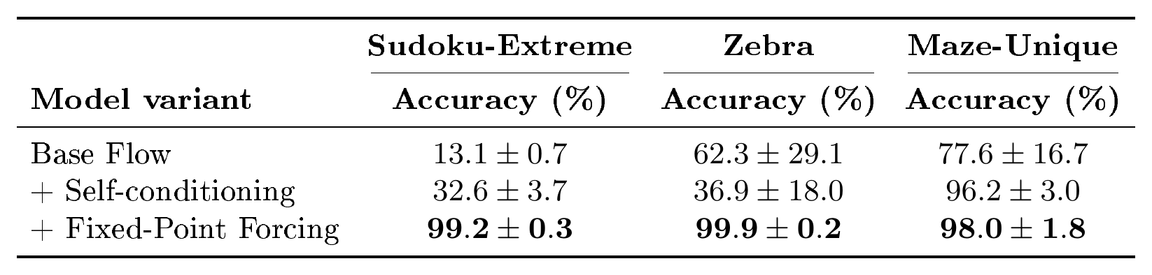
Across all three tasks, the vanilla FLM baselines plateau well below the full FRM (Table 2), and allocating more forward passes leaves their solve-rate curves essentially flat. Additional integration more accurately traces the learned probability path, but provides no mechanism for repeatedly revising the current solution.
Self-conditioning enables recurrent refinement.
Adding self-conditioning improves solve rate over a plain discrete flow on Sudoku-Extreme ($13.1% \rightarrow 32.6%$) and Maze-Unique ($77.6% \rightarrow 96.2%$; Table 2). On Zebra, however, self-conditioning lowers the three-seed mean from $62.3%$ to $36.9%$, and both the base and self-conditioned flows exhibit high seed variance. Feeding each prediction back to the model creates a recurrent computation that can preserve correct assignments and revise earlier mistakes, as illustrated by the decoded trajectory in Figure 2. On an easier Sudoku variant introduced by [19] (Sudoku-Shah), self-conditioning alone is already sufficient to raise solve rate from approximately $30%$ to $99%$, showing that recurrent refinement can saturate less demanding constraint problems without Fixed-Point Forcing.
Conventional self-conditioning remains unreliable at depth.
Despite these gains, its Sudoku-Extreme solve rate plateaus near one-third of puzzles as recurrent depth increases (Figure 6 b), motivating a training procedure that makes the recurrent computation reliable over long rollouts.
4.3 Fixed-Point Forcing Creates Healthy Reasoning Dynamics
Exposure bias produces confidently incorrect fixed points.
With conventional self-conditioning, solve rate plateaus as recurrent depth increases while gold-target cross-entropy grows even as the adjacent-state symmetric-KL residual shrinks (Figure 6 a, b). The model is therefore not simply failing to converge: it is becoming increasingly confident in self-consistent but incorrect predictions. Correspondingly, residual magnitude is uninformative about correctness (AUROC $0.50$; Figure 6 c).
Fixed-Point Forcing mitigates exposure bias, enabling recurrent test-time scaling.
Replacing the one-pass training carry with a rollout-derived carry raises the three-seed mean solve rate from $32.6%$ to $99.2%$ on Sudoku-Extreme and from $96.2%$ to $98.0%$ on Maze-Unique. On Zebra, the three FPF seeds average $99.9%$ (Table 2); the best evaluated operating points reach $99.5%$ on Sudoku-Extreme and $99.9%$ on Maze-Unique (Table 1). More importantly, conventional self-conditioning plateaus with recurrent depth, whereas FPF continues converting additional model evaluations into corrected solutions (Figure 6 b). Because FPF changes the training distribution of recurrent carries while preserving the architecture, canonical flow path, and endpoint objective, the comparison isolates exposure to inference-induced states as the intervention that unlocks recurrent test-time scaling.
Fixed-Point Forcing aligns convergence with correctness.
Under FPF, additional recurrent updates reduce gold-target cross-entropy as solve rate increases, directing convergent trajectories toward the correct solution rather than merely toward a self-consistent prediction (Figure 6 a, b). We measure convergence by the token-averaged symmetric KL between adjacent predictive distributions, $r_k=D_{\mathrm{SKL}}(p_k, p_{k-1})$. This residual changes from a chance-level correctness signal under conventional self-conditioning to a nearly perfect one under FPF (AUROC $1.00$; Figure 6 c). Convergence thus becomes an observable signature of successful reasoning, although not a formal certificate of correctness. Together, these findings support the attractor picture in Figure 1: conventional self-conditioning admits stable incorrect fixed points, whereas FPF reshapes the closed-loop dynamics so that correct solutions behave as stable, error-correcting attractors. The depicted basins summarize this empirical dynamical behavior rather than asserting a literal low-dimensional geometry.
::: {caption="Table 2: Training-recipe ablation across three reasoning tasks. Entries report the mean ± sample standard deviation over three training seeds. For each seed, we select the checkpoint and inference configuration with the highest validation solve rate."}
:::
5. Related Work
Section Summary: Recent work has explored diffusion and flow models as non-autoregressive alternatives for generating text, often using iterative denoising or probability paths to produce sequences. Separate lines of research have developed recurrent architectures that reuse the same weights over multiple steps to scale up reasoning at test time and converge on answers through attractor dynamics. FRMs connect these threads by treating a flow model’s clean predictions as both recurrent state and explicit solution, while training on the model’s own generated states to avoid exposure bias without needing specialized architectures or backpropagation through rollouts.
Diffusion and Flow Language Models.
A substantial body of work has developed diffusion-based alternatives to autoregressive modeling for discrete data and language ([11, 12, 13]). Masked Diffusion Language Models generate sequences through iterative denoising ([1]). [20] derive a simplified continuous-time objective as a weighted integral of cross-entropy losses and generalize the framework to state-dependent masking schedules. Within this family, [2] use adaptive token ordering to allocate computation, whereas [16] introduce remasking so earlier commitments can be revised; Duo instead uses uniform categorical corruption, keeping every token revisable throughout sampling ([21]). More recently, continuous flow language models have emerged as competitive alternatives. FLM learns Gaussian-to-one-hot probability paths and FMLM distills them into few-step maps ([4]), while LangFlow and ELF define flows in learned and contextual embedding spaces, respectively ([22, 5]). FRMs are inspired by this diffusion-and-flow tradition, but use the clean denoiser prediction as a directly decodable recurrent state and train the resulting closed loop for iterative solution refinement rather than treating repeated evaluations only as steps of a generative sampler.
Recurrent and Fixed-Point Reasoning.
Recent structured reasoners scale test-time computation through weight-tied recurrence. HRM uses hierarchical recurrent states ([6]). TRM ([17]) and PTRM ([23]) repeatedly update compact answer and latent states. EqR explicitly trains solution-aligned attractor dynamics ([10]). FPRM similarly observes that convergence becomes predictive of correctness and uses this signal for adaptive halting ([18]). FRMs share the emphasis on recurrent test-time scaling, attractor dynamics, and meaningful convergence, but realize them within a self-conditioned flow language model: the flow denoiser's clean prediction is both the recurrent input and an explicit solution candidate. Rather than introducing a bespoke latent-state architecture, FRM retains the standard non-causal Transformer and flow objective already demonstrated at language-model scale ([4, 5]), providing a natural path toward larger models and less specialized domains. FPF further avoids backpropagation through the rollout: model-generated states enter only through the conditioning channel, while every loss-bearing flow state remains on the target-derived canonical path.
Learning from Model-Induced States.
Conventional self-conditioning feeds a detached estimate of the clean sample into later denoising steps, but trains that channel with a one-pass prediction rather than the recursively generated predictions encountered during inference, as introduced for continuous encodings of discrete data by Analog Bits ([7]). This is an instance of exposure bias: the model is evaluated on its own induced context without being trained on that context ([24, 8]). Concurrent work likewise frames self-conditioned flow language models as fixed-point iterations for few-step generation ([25]); we study structured reasoning and training on model-induced recurrent states. Self Forcing closes the analogous context mismatch in autoregressive video diffusion by training on self-generated rollout context ([9]). FPF can be understood as a self-forcing variant specialized to the recurrent conditioning channel of conditional discrete flows: it treats the carry, rather than previous frames, as model-generated context. Unlike Self Forcing, FPF requires neither a sequence-level distribution-matching objective nor differentiation through the rollout; it changes only the carry distribution while preserving the canonical flow path and endpoint objective.
6. Discussion
Section Summary: Flow Reasoning Models show that discrete flow-based systems can handle structured reasoning tasks like puzzles, logical deductions, and pathfinding with strong results and efficient use of computation. By repeatedly conditioning on their own earlier outputs and training with a technique called Fixed-Point Forcing, these models develop an iterative refinement process that improves accuracy without needing specially designed recurrent components. The findings indicate that general-purpose generative models can produce effective step-by-step reasoning through learned dynamics, though scaling them to bigger and messier problems remains an open challenge.
Flow Reasoning Models indicate that discrete flows can be a powerful and efficient model class for structured reasoning. Across constraint satisfaction, relational deduction, and path finding, FRMs achieve strong performance while retaining a favorable accuracy–compute tradeoff. Conditioning discrete flows on their own past predictions creates an iterative refinement process, while training on recursively generated states with Fixed-Point Forcing dramatically improves performance and makes additional recurrent depth productive. Together, these results suggest that recurrent reasoning need not rely on a specialized recurrent architecture: it can emerge from the learned refinement dynamics of a general-purpose generative model. Scaling this approach to larger models and less structured tasks is an important direction for future work.
Appendix
Section Summary: The appendix details the experimental setup for evaluating reasoning models on three specialized benchmarks. Sudoku-Extreme tests complex puzzle solving with 9x9 grids, Zebra examines relational logic across varying house-attribute puzzles, and Maze-Unique assesses unique pathfinding in 30x30 grids, each with fixed training splits, augmentations, and exact solution accuracy as the metric. It also outlines the shared DiT model architecture, two-stage training process with self-conditioning and refinement steps, dataset-specific hyperparameters, and how baseline comparisons from autoregressive, diffusion, and recurrent models were sourced and evaluated for fair assessment.
A. Experimental Details
A.1 Datasets
Sudoku-Extreme.
We use Sudoku-Extreme to test long-horizon constraint satisfaction on hard $9\times9$ puzzles that require extended chains of deduction and search. The benchmark was introduced with the Hierarchical Reasoning Model as a small-data test of recurrent reasoning ([6]); we represent each released puzzle as its unique solution together with a mask that clamps the given clues. For each training seed, we draw a difficulty-balanced subset of 1, 000 puzzles from the official training split and apply random Sudoku symmetries as augmentation. We select checkpoints on a fixed held-out validation subset and report exact-grid solve rate on a fixed 1, 000-puzzle subset of the official test split.
Zebra.
We use Zebra to test whether recurrent refinement transfers from grid-local constraints to heterogeneous relational reasoning. Introduced as a reasoning benchmark by [19], the dataset contains approximately 1.5 million training and 0.1 million test instances spanning three to six houses and attributes. Following the uniform $3\times3$ – $6\times6$ mixture introduced by [19] and used by [2], we train and evaluate across all four puzzle sizes rather than restricting the benchmark to a fixed $5\times5$ slice. We retain each puzzle's original clue serialization but replace its variable, solver-ordered trace with a canonical attribute-by-house solution grid. We report exact-grid solve rate on the mixed held-out split.
Maze-Unique.
We use Maze-Unique to test structured path finding under an unambiguous exact-solve criterion. Released with Equilibrium Reasoners ([10]), this $30\times30$ path-finding benchmark provides official, revision-pinned splits of 1, 000 training and 1, 000 test mazes; we encode walls, start, and goal as clamped cells and generate the remainder of the grid. We prefer it to the more common Maze-Hard benchmark because every instance has a unique solution path, making exact-grid accuracy coincide with path validity and optimality instead of penalizing an alternative valid route. It also permits direct comparison with recent recurrent reasoners evaluated on the same split.
A.2 Models and Training
All experiments use a non-causal DiT backbone and the categorical clean-prediction objective. AdamW with $\beta=(0.9, 0.999)$, gradient clipping at $1.0$, EMA decay $0.9999$, dropout $0.1$, and a constant learning-rate schedule are shared across datasets. The learning rate, weight decay, batch size, warmup, training budget, and architecture vary by dataset and are reported in Table 3. In every case, Stage A trains self-conditioning from scratch; Stage B initializes from the selected Stage-A weights with a fresh optimizer and EMA state before applying FPF. For each training seed, we select the checkpoint and inference configuration (including sampler and NFE) with the highest validation solve rate. Table 2 aggregates the resulting selected operating points across seeds.
\begin{tabular*}{\ccccccccc}{@{\extracolsep{\fill}}lccc@}
  \toprule
  \textbf{Setting} & \textbf{Sudoku-Extreme} & Zebra $3\times3$-- $6\times6$ & \textbf{Maze-Unique} \\
  \midrule
  \multicolumn{4}{l}{\textit{Architecture}} \\
  Parameters & $7.0$ M & $25.0$ M & $8.0$ M \\
  Hidden size / blocks / heads & $256$ / $7$ / $8$ & $384$ / $12$ / $12$ & $256$ / $8$ / $8$ \\
  Sequence length / vocabulary & $81$ / $10$ & size-dependent / $21$ & $900$ / $6$ \\
  \midrule
  \multicolumn{4}{l}{\textit{Optimization}} \\
  Optimizer / betas & AdamW / $(0.9, 0.999)$ & AdamW / $(0.9, 0.999)$ & AdamW / $(0.9, 0.999)$ \\
  Learning rate / weight decay & $3\times10^{-4}$ / $0$ & $3\times10^{-4}$ / $0$ & $1\times10^{-4}$ / $1.0$ \\
  Global batch size per step & $128$ & $128$ & $64$ \\
  Warmup steps & $0$ & $0$ & $500$ \\
  Gradient clip & $1.0$ & $1.0$ & $1.0$ \\
  EMA decay & $0.9999$ & $0.9999$ & $0.9999$ \\
  Dropout & $0.1$ & $0.1$ & $0.1$ \\
  Learning-rate schedule & constant & constant & constant \\
  Stage-A / Stage-B iterations & $100$ K / $100$ K & $200$ K / $200$ K & $300$ K / $100$ K \\
  \midrule
  \multicolumn{4}{l}{\textit{Self-conditioning and FPF}} \\
  Self-conditioning probability & $0.5$ & $0.5$ & $0.5$ \\
  FPF rollout probability / depth & $0.5$ / $16$ & $0.5$ / $16$ & $0.5$ / $16$ \\
  Supervised states / noise scale & $4$ / $0$ & $4$ / $0$ & $4$ / $0$ \\
  \bottomrule
  \end{tabular*}
A.3 Baseline Provenance and Comparability
We organize baselines into three families because they make different architectural commitments. The autoregressive baseline is a plain causal decoder-only transformer trained with teacher-forced next-token cross-entropy over a clue-grid-then-solution-grid sequence: no denoising, no recurrence, and no mechanism to revise an already-committed token, making it the naive baseline the rest of the comparison is meant to contextualize ([19]). Diffusion language models and flows use a general-purpose generative denoising formulation that can share the same non-causal DiT backbone as FRM. Small recurrent reasoning models instead introduce task-oriented recurrent state, update, or halting mechanisms. This grouping clarifies the role of each comparison; it does not by itself imply matched capacity or compute, so Table 1 reports the model size used on each benchmark and Appendix A.4 reports inference cost.
Accuracy provenance.
Unless noted here, entries in Table 1 are measurements from our evaluation harness using checkpoints that we trained or official checkpoints that we evaluated. For Zebra, the FMLM, FLM, and FRM entries are our measurements. The daggered MDLM and adaptive-MDLM accuracies are published values from [2] on Shah's uniform $3\times3$ – $6\times6$ mixture; we could not reproduce those reported accuracies in our pipeline. Our weight-backed Zebra MDLM reproduction peaks at $49.2%$ under our shorter training budget and supplies the measured operating points used for efficiency analysis. We omit ReMDM and specialized recurrent reasoners on Zebra because we did not obtain a reliable result under the same mixed protocol; the dashes therefore indicate unavailable comparisons, not zero accuracy. For Maze-Unique, EqR is a published reference value, whereas TRM is our $0.264$ M-parameter reproduction trained and evaluated on the Maze-Unique split, reaching $77.9%$ exact solve rate. The $44.9%$ result reported by the original TRM work is for Maze-Hard, not Maze-Unique, and is therefore excluded from this table. The remaining Maze-Unique entries are measured from our trained reproductions or evaluated checkpoints. Thus, published accuracies support the headline comparison, whereas every point in an accuracy–compute frontier is produced from a checkpoint available to our profiler.
A.4 Inference Compute Accounting
Number of function evaluations.
We report the realized number of learned-model evaluations required to solve one puzzle. For our Euler, SDE, and held-time samplers, NFE counts every iterative update and the final readout evaluation; for methods with adaptive stopping, branching, or breadth, we count all evaluations actually executed for that instance. NFE exposes the number of sequential model calls and is easy to reproduce, but it is not a sufficient cross-method compute measure: one evaluation can differ substantially in cost across architectures, sequence lengths, model sizes, and internally recurrent networks. The appendix table reports solved-puzzle mean NFE: for each puzzle that is solved at some point along its evaluated trajectory, we record the first NFE at which it is solved and average over solved puzzles only. This is an oracle trajectory diagnostic unless correctness can be detected without access to the ground truth; it should therefore not be interpreted as deployable early stopping for every method.
Floating-point operations.
We therefore use total FLOPs per puzzle as the primary hardware-independent compute measure. We profile an actual batch-one forward pass with PyTorch's operator-level FLOP counter, disabling fused attention so that its matrix multiplications are visible, and multiply the measured per-evaluation cost by the realized NFE; methods with nonuniform calls are profiled and summed by call type. This quantity should be interpreted as a lower bound on the work required to solve an instance: it counts floating-point arithmetic but not memory traffic, kernel-launch and framework overhead, control flow, communication, or data movement. We therefore present the full accuracy–compute frontiers rather than compressing each method to a single operating-point ratio.
B. Additional Accuracy and Ablation Results
This section documents the headline accuracy–compute comparison and training-recipe ablation; Appendix A gives datasets, checkpoint provenance, and FLOP accounting.
B.1 Accuracy–Compute Evaluation
Each frontier contains measured operating points only. We vary each checkpoint's native compute control and charge every learned-model call. Fixed-depth methods use the requested depth; adaptive methods use realized mean computation. We neither extrapolate unsupported method–dataset pairs nor include published accuracies lacking a compatible profiled checkpoint, although those values may still appear in Table 1.
: Table 4: Inference controls used to construct accuracy–compute frontiers. Every learned-model invocation is included in the reported computation. Exact evaluated grids are checkpoint- and dataset-specific.
| Method | Inference-time control | Charged computation |
|---|---|---|
| FMLM / FLM | Flow-integration steps | All denoiser evaluations |
| MDLM | Denoising steps | All denoiser evaluations |
| ReMDM | Denoising and remasking steps | All denoiser and remasking evaluations |
| Adaptive MDLM | Update cap and confidence rule | Realized adaptive evaluations |
| HRM / TRM / FPRM | Recurrent depth | All recurrent model evaluations |
| EqR | Equilibrium depth and breadth | All iterations and evaluated branches |
| FRM (ours) | Recurrent depth and sampler | All recurrent denoiser evaluations |
Adaptive computation.
Token-adaptive methods can incur a nonzero minimum cost even at their lowest nominal setting. We therefore plot measured realized FLOPs rather than the maximum-step label.
B.2 Training-Recipe Results
Table 2 reports three-seed means and standard deviations for every dataset. We report aggregate statistics consistently and omit individual-seed values.
C. Additional Dynamics Analysis
We distinguish productive refinement from convergence to an incorrect fixed point using the following depth-dependent diagnostics.
Depth-dependent performance and distance to the solution.
At each depth, we record exact solve rate and token-averaged cross-entropy to the one-hot solution on the same pinned examples. Thus changes isolate additional recurrent computation. In Figure 6, FPF improves accuracy while driving ground-truth loss downward; conventional self-conditioning becomes increasingly confident in incorrect states.
Convergence residual and correctness prediction.
For adjacent distributions $p_k$ and $p_{k-1}$, we measure the token-averaged symmetric-KL residual $r_k=D_{\mathrm{SKL}}(p_k, p_{k-1})$ and pair it with the decoded state's exact-solve label. A near-zero residual indicates convergence, not necessarily correctness. Conventional self-conditioning yields chance-level discrimination (AUROC $0.50$); under FPF, convergence is strongly predictive of correctness (AUROC $1.00$) on Sudoku-Extreme.
Interpretation.
Exact solve rate remains primary; loss-to-gold and adjacent-state residuals reveal whether depth corrects the solution or settles into a confidently incorrect fixed point.
References
Section Summary: This section compiles a list of academic papers and preprints that serve as sources for the document. Most are recent works from 2024–2026 on arXiv, focusing on diffusion models, flow matching, and related techniques for generating language and discrete data, with a smaller number of earlier conference papers on sequence modeling and training methods. Together they trace the key technical developments and prior research underpinning the main text.
[1] Subham Sekhar Sahoo et al. (2024). Simple and Effective Masked Diffusion Language Models. https://arxiv.org/abs/2406.07524. arXiv:2406.07524.
[2] Jaeyeon Kim et al. (2025). Train for the Worst, Plan for the Best: Understanding Token Ordering in Masked Diffusions. https://arxiv.org/abs/2502.06768. arXiv:2502.06768.
[3] Guanghan Wang et al. (2026). Remasking Discrete Diffusion Models with Inference-Time Scaling. https://arxiv.org/abs/2503.00307. arXiv:2503.00307.
[4] Chanhyuk Lee et al. (2026). Flow Map Language Models: One-step Language Modeling via Continuous Denoising. https://arxiv.org/abs/2602.16813. arXiv:2602.16813.
[5] Keya Hu et al. (2026). ELF: Embedded Language Flows. https://arxiv.org/abs/2605.10938. arXiv:2605.10938.
[6] Guan Wang et al. (2025). Hierarchical Reasoning Model. https://arxiv.org/abs/2506.21734. arXiv:2506.21734.
[7] Ting Chen et al. (2023). Analog Bits: Generating Discrete Data using Diffusion Models with Self-Conditioning. https://arxiv.org/abs/2208.04202. arXiv:2208.04202.
[8] Samy Bengio et al. (2015). Scheduled Sampling for Sequence Prediction with Recurrent Neural Networks. In Advances in Neural Information Processing Systems. https://proceedings.neurips.cc/paper/2015/hash/e995f98d56967d946471af29d7bf99f1-Abstract.html.
[9] Xun Huang et al. (2025). Self Forcing: Bridging the Train-Test Gap in Autoregressive Video Diffusion. https://arxiv.org/abs/2506.08009. arXiv:2506.08009.
[10] Benhao Huang et al. (2026). Equilibrium Reasoners: Learning Attractors Enables Scalable Reasoning. https://arxiv.org/abs/2605.21488. arXiv:2605.21488.
[11] Jacob Austin et al. (2021). Structured Denoising Diffusion Models in Discrete State-Spaces. In Advances in Neural Information Processing Systems. pp. 17981–17993. https://proceedings.neurips.cc/paper/2021/hash/958c530554f78bcd8e97125b70e6973d-Abstract.html.
[12] Itai Gat et al. (2024). Discrete Flow Matching. In Advances in Neural Information Processing Systems. pp. 133345–133385. doi:10.52202/079017-4239. https://proceedings.neurips.cc/paper_files/paper/2024/hash/f0d629a734b56a642701bba7bc8bb3ed-Abstract-Conference.html.
[13] Hannes Stark et al. (2024). Dirichlet Flow Matching with Applications to DNA Sequence Design. In Proceedings of the 41st International Conference on Machine Learning. pp. 46495–46513. https://proceedings.mlr.press/v235/stark24b.html.
[14] Yaron Lipman et al. (2023). Flow Matching for Generative Modeling. In International Conference on Learning Representations. https://openreview.net/forum?id=PqvMRDCJT9t.
[15] Michael S. Albergo et al. (2025). Stochastic Interpolants: A Unifying Framework for Flows and Diffusions. Journal of Machine Learning Research. 26(209). pp. 1–80. https://www.jmlr.org/papers/v26/23-1605.html.
[16] Guanghan Wang et al. (2025). Remasking Discrete Diffusion Models with Inference-Time Scaling. In Advances in Neural Information Processing Systems. pp. 147282–147339. doi:10.52202/085713-4927. https://proceedings.neurips.cc/paper_files/paper/2025/hash/d877ea0dd78bdbe54830670618c1de09-Abstract-Conference.html.
[17] Alexia Jolicoeur-Martineau (2025). Less is More: Recursive Reasoning with Tiny Networks. https://arxiv.org/abs/2510.04871. arXiv:2510.04871.
[18] Sajad Movahedi et al. (2026). Fixed-Point Reasoners: Stable and Adaptive Deep Looped Transformers. https://arxiv.org/abs/2606.18206. arXiv:2606.18206.
[19] Kulin Shah et al. (2024). Causal Language Modeling Can Elicit Search and Reasoning Capabilities on Logic Puzzles. https://arxiv.org/abs/2409.10502. arXiv:2409.10502.
[20] Jiaxin Shi et al. (2025). Simplified and Generalized Masked Diffusion for Discrete Data. https://arxiv.org/abs/2406.04329. arXiv:2406.04329.
[21] Subham Sekhar Sahoo et al. (2025). The Diffusion Duality. arXiv preprint arXiv:2506.10892. https://arxiv.org/abs/2506.10892.
[22] Yuxin Chen et al. (2026). LangFlow: Continuous Diffusion Rivals Discrete in Language Modeling. https://arxiv.org/abs/2604.11748. arXiv:2604.11748.
[23] Amin Sghaier et al. (2026). Probabilistic Tiny Recursive Model. https://arxiv.org/abs/2605.19943. arXiv:2605.19943.
[24] Stéphane Ross et al. (2011). A Reduction of Imitation Learning and Structured Prediction to No-Regret Online Learning. In Proceedings of the Fourteenth International Conference on Artificial Intelligence and Statistics. pp. 627–635. https://proceedings.mlr.press/v15/ross11a.html.
[25] Jaehoon Yoo et al. (2026). Self-conditioned Flow Map Language Models via Fixed-point Flows. https://arxiv.org/abs/2607.00714. arXiv:2607.00714.