Modeling Indirect Illumination for Inverse Rendering

Yuanqing ZhangJiaming SunXingyi HeHuan FuRongfei JiaXiaowei Zhou

article2022CVPR231 citations

Presents an efficient inverse rendering framework that derives indirect illumination directly from a pre-trained neural radiance field, bypassing costly path tracing to recover accurate, shadow- and interreflection-free material properties from multi-view images under unknown lighting.

Listen

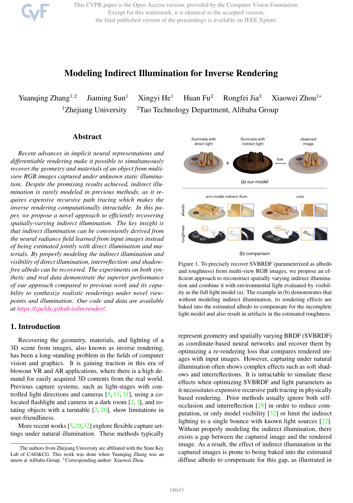
The rapid growth of virtual and augmented reality applications demands practical techniques to digitize real-world objects into relightable 3D assets. Inverting standard photographs into geometry, material reflectance, and lighting parameters—known as inverse rendering—is notoriously difficult under casual capture conditions. Previous approaches typically ignore indirect illumination, such as interreflections between object surfaces, because simulating multiple light bounces through recursive ray tracing requires prohibitive computational resources. Consequently, prior methods suffer from significant rendering errors, erroneously embedding reflected light and shadows into the estimated surface colors.

The article demonstrates a computationally efficient inverse rendering framework that recovers precise object geometry, material reflectance, and environmental lighting from multi-view photographs captured under unknown, static illumination. The core objective is to model complex indirect illumination and direct light occlusion without resorting to expensive recursive path tracing.

To achieve this, the approach breaks the problem into a three-stage workflow using coordinate-based neural networks. First, it reconstructs the 3D surface geometry and the outgoing radiance field from multi-view imagery. Next, it derives indirect illumination directly from this pre-trained radiance field, caching the incoming light and direct visibility into dedicated neural networks represented as spherical mathematical functions. Finally, the framework jointly optimizes the material properties—modeled via a sparse autoencoder that enforces realistic material consistency—and direct environmental lighting. The method was evaluated using four multi-material synthetic 3D models with prominent self-occlusions across standard perceptual and reconstruction quality metrics, alongside real-world video captures of everyday objects taken with a mobile phone.

The analysis yields several key findings. First, explicitly modeling indirect illumination prevents interreflections and soft shadows from baking into the estimated surface albedo, yielding clean, true-to-life diffuse colors. Second, the method achieved superior material decomposition and relighting accuracy compared to existing baselines, achieving higher peak signal-to-noise ratios (25.59 dB versus 21.54 dB for NeRFactor and 22.63 dB for modified PhySG in relighting tests). Third, the sparsity constraint on the material network successfully reduced surface roughness noise, avoiding the overfitting that commonly occurs when optimizing surface points independently. Fourth, training required only about three hours on a single consumer-grade graphics processing unit (NVIDIA RTX 3090) across the final two stages, confirming high computational efficiency.

These findings indicate that high-fidelity 3D asset digitisation can be achieved using accessible hardware and casual capture settings, substantially reducing production costs and turnaround times for graphics pipelines. By successfully disentangling material reflectance from incoming light, the method allows recovered 3D objects to be realistically placed and relit under completely novel lighting environments without visual artifacts.

Organizations seeking to digitize real-world physical assets should adopt indirect-illumination-aware neural inverse rendering pipelines for 3D reconstruction tasks. When implementing this method, practitioners must ensure high-quality initial multi-view captures with accurate camera poses, as the pipeline relies heavily on successful upstream geometry estimation. Future technical development should focus on extending the material formulation beyond dielectric assumptions to support metallic surfaces by learning variable Fresnel coefficients.

Cover for Modeling Indirect Illumination for Inverse Rendering

Abstract

Recent advances in implicit neural representations and differentiable rendering make it possible to simultaneously recover the geometry and materials of an object from multi-view RGB images captured under unknown static illumination. Despite the promising results achieved, indirect illumination is rarely modeled in previous methods, as it requires expensive recursive path tracing which makes the inverse rendering computationally intractable. In this paper, we propose a novel approach to efficiently recovering spatially-varying indirect illumination. The key insight is that indirect illumination can be conveniently derived from the neural radiance field learned from input images instead of being estimated jointly with direct illumination and materials. By properly modeling the indirect illumination and visibility of direct illumination, interreflection- and shadow-free albedo can be recovered. The experiments on both synthetic and real data demonstrate the superior performance of our approach compared to previous work and its capability to synthesize realistic renderings under novel viewpoints and illumination. Our code and data are available at https://zju3dv.github.io/invrender/.

Table of Contents

  • 1. Introduction
  • 2. Background
  • 3. Method
  • 3.1. Overview
  • 3.2. Visibility for Direct Illumination
  • 3.3. Indirect Illumination
  • 3.4. BRDF
  • 3.5. Rendering
  • 3.6. Training
  • 4. Experiments
  • 4.1. Synthetic Data
  • 4.2. Baseline Comparisons
  • 4.3. Ablation Studies
  • 4.4. Results on Real Captures.
  • 5. Conclusion
  • References

Knowls

  1. Knowl 1 — Indirect Illumination Modeling via Neural Radiance Field Caching

    model/method

    In inverse rendering, indirect incoming radiance at a surface point x^\hat{\mathbf{x}} along direction ωi\boldsymbol{\omega}_i corresponds to the outgoing radiance Lo(x^′,−ωi)L_o(\hat{\mathbf{x}}', -\boldsymbol{\omega}_i) from a secondary intersection point x^′\hat{\mathbf{x}}':

    Li(x^,ωi)=Lo(x^′,−ωi)L_i(\hat{\mathbf{x}}, \boldsymbol{\omega}_i) = L_o(\hat{\mathbf{x}}', -\boldsymbol{\omega}_i)

    Instead of performing costly recursive ray tracing during the optimization of materials and lighting, the indirect illumination is derived directly from a pre-trained neural outgoing radiance field R(x^′,n^′,−ωi)↦LoR(\hat{\mathbf{x}}', \hat{\mathbf{n}}', -\boldsymbol{\omega}_i) \mapsto L_o, where n^′\hat{\mathbf{n}}' is the surface normal at x^′\hat{\mathbf{x}}'. This radiance field is learned jointly with the surface geometry Signed Distance Function (SDF) from multi-view images.

    To avoid repeated ray tracing from x^\hat{\mathbf{x}} to x^′\hat{\mathbf{x}}' during inverse rendering, the indirect illumination is distilled and cached into an indirect illumination multilayer perceptron (MLP) I(x)I(\mathbf{x}). For any 3D coordinate x\mathbf{x}, I(x)I(\mathbf{x}) outputs the parameters of a mixture of 24 Spherical Gaussians (SGs), Γ∈R24×7\boldsymbol{\Gamma} \in \mathbb{R}^{24 \times 7} (where each SG has a 3D lobe axis ξ∈S2\boldsymbol{\xi} \in \mathbb{S}^2, a 1D sharpness λ∈R+\lambda \in \mathbb{R}^+, and a 3D RGB amplitude μ∈R3\boldsymbol{\mu} \in \mathbb{R}^3):

    Li(x^,ωi)=G(ωi;I(x^))L_i(\hat{\mathbf{x}}, \boldsymbol{\omega}_i) = G(\boldsymbol{\omega}_i; I(\hat{\mathbf{x}}))

    The network I(x)I(\mathbf{x}) is supervised by querying incoming rays against the pre-trained neural radiance field RR using an ℓ1\ell_1 loss and is subsequently fixed during the optimization of spatially varying BRDF and direct environment illumination.

  2. Knowl 2 — Direct Illumination and Spherical Gaussian Visibility Approximation

    model/method

    Direct illumination is assumed to originate from an infinitely distant environment and is parameterized as a mixture of M=128M = 128 Spherical Gaussians (SGs):

    E(ωi)=∑k=1MG(ωi;ξk,λk,μk)E(\boldsymbol{\omega}_i) = \sum_{k=1}^{M} G(\boldsymbol{\omega}_i; \boldsymbol{\xi}_k, \lambda_k, \boldsymbol{\mu}_k)

    where ξk∈S2\boldsymbol{\xi}_k \in \mathbb{S}^2 is the lobe axis, λk∈R+\lambda_k \in \mathbb{R}^+ is the lobe sharpness, and μk∈R3\boldsymbol{\mu}_k \in \mathbb{R}^3 is the lobe amplitude.

    To evaluate self-occlusion efficiently without executing sphere tracing at every rendering step, light visibility is re-parameterized as a continuous MLP V(x,ωi)↦v∈[0,1]V(\mathbf{x}, \boldsymbol{\omega}_i) \mapsto v \in [0, 1] mapping a 3D location x\mathbf{x} and incident direction ωi\boldsymbol{\omega}_i to a visibility scalar.

    The direction-wise product of visibility and an incident lighting SG is approximated by scaling the SG's amplitude by an integrated visibility ratio γ\gamma, preserving the lobe center and sharpness:

    V(x,ωi)⊗G(ωi;ξ,λ,μ)≈G(ωi;ξ,λ,γμ)V(\mathbf{x}, \boldsymbol{\omega}_i) \otimes G(\boldsymbol{\omega}_i; \boldsymbol{\xi}, \lambda, \boldsymbol{\mu}) \approx G(\boldsymbol{\omega}_i; \boldsymbol{\xi}, \lambda, \gamma \boldsymbol{\mu})

    where γ\gamma is computed by taking a weighted average over S=32S = 32 directions sampled within the SG lobe:

    γ=∑k=1SG(ωk)V(x,ωk)∑k=1SG(ωk)\gamma = \frac{\sum_{k=1}^S G(\boldsymbol{\omega}_k) V(\mathbf{x}, \boldsymbol{\omega}_k)}{\sum_{k=1}^S G(\boldsymbol{\omega}_k)}

  3. Knowl 3 — Sparse Latent Space BRDF Representation

    model/method

    To constrain the inverse rendering problem and reflect the prior that real-world objects consist of a small number of distinct materials, spatially varying BRDF (SVBRDF) parameters—diffuse albedo a∈[0,1]3\mathbf{a} \in [0, 1]^3 and roughness r∈[0,1]r \in [0, 1] from the Disney BRDF model with fixed dielectric Fresnel reflectance F0=0.02F_0 = 0.02—are parameterized using an encoder-decoder neural network with a sparse latent space.

    The encoder maps a 3D surface position x\mathbf{x} to an nn-dimensional latent code z∈R32\mathbf{z} \in \mathbb{R}^{32}. A sparsity constraint enforces that most latent channels remain near zero via a Kullback-Leibler (KL) divergence loss:

    ℓKL=∑j=1nKL(ρ∥ρ^j)=∑j=1n(ρlog⁡ρρ^j+(1−ρ)log⁡1−ρ1−ρ^j)\ell_{\mathrm{KL}} = \sum_{j=1}^{n} \mathrm{KL}(\rho \parallel \hat{\rho}_j) = \sum_{j=1}^{n} \left( \rho \log \frac{\rho}{\hat{\rho}_j} + (1 - \rho) \log \frac{1 - \rho}{1 - \hat{\rho}_j} \right)

    where ρ^j\hat{\rho}_j denotes the batch average activation of the jj-th latent channel and ρ=0.05\rho = 0.05 is the target sparsity parameter.

    The decoder DD maps latent code z\mathbf{z} to albedo a\mathbf{a} and roughness rr. A local smoothness regularizer clusters nearby latent codes to output identical material parameters:

    ℓs=∥D(z)−D(z+ξ)∥1\ell_s = \| D(\mathbf{z}) - D(\mathbf{z} + \boldsymbol{\xi}) \|_1

    where ξ∼N(0,0.012I)\boldsymbol{\xi} \sim \mathcal{N}(\mathbf{0}, 0.01^2 \mathbf{I}) is a random Gaussian perturbation.

  4. Knowl 4 — Differentiable Spherical Gaussian Forward Rendering

    model/method

    The forward rendering equation computes outgoing radiance Lo(x^,ωo)L_o(\hat{\mathbf{x}}, \boldsymbol{\omega}_o) along view direction ωo\boldsymbol{\omega}_o at surface point x^\hat{\mathbf{x}} with surface normal n=∇x^S\mathbf{n} = \nabla_{\hat{\mathbf{x}}} S by integrating incoming light over the upper hemisphere Ω\Omega:

    Lo(x^,ωo)=∫ΩLin(x^,ωi)fr(x^,ωi,ωo)(ωi⋅n)dωiL_o(\hat{\mathbf{x}}, \boldsymbol{\omega}_o) = \int_\Omega L_{\mathrm{in}}(\hat{\mathbf{x}}, \boldsymbol{\omega}_i) f_r(\hat{\mathbf{x}}, \boldsymbol{\omega}_i, \boldsymbol{\omega}_o) (\boldsymbol{\omega}_i \cdot \mathbf{n}) \mathrm{d}\boldsymbol{\omega}_i

    The BRDF frf_r consists of a diffuse component aπ\frac{\mathbf{a}}{\pi} and a specular component fs(x^,ωi,ωo)f_s(\hat{\mathbf{x}}, \boldsymbol{\omega}_i, \boldsymbol{\omega}_o). Both the specular BRDF lobe fsf_s and the clamped cosine term C=max⁡(ωi⋅n,0)C = \max(\boldsymbol{\omega}_i \cdot \mathbf{n}, 0) are converted to single Spherical Gaussians (SGs), allowing hemispherical integrals to be evaluated analytically via fast inner products of SGs.

    Direct illumination rendering decomposes into a diffuse term LdL_d and a specular term LsL_s across MM environment lighting SGs Ek(ωi)E_k(\boldsymbol{\omega}_i):

    Ld(x^)=aπ∑k=1M(V(x^,ωi)⊗Ek(ωi))⋅CL_d(\hat{\mathbf{x}}) = \frac{\mathbf{a}}{\pi} \sum_{k=1}^M \left( V(\hat{\mathbf{x}}, \boldsymbol{\omega}_i) \otimes E_k(\boldsymbol{\omega}_i) \right) \cdot C

    Ls(x^,ωo)=∑k=1M(fs⊗V(x^,ωi))⊗Ek(ωi)⋅CL_s(\hat{\mathbf{x}}, \boldsymbol{\omega}_o) = \sum_{k=1}^M \left( f_s \otimes V(\hat{\mathbf{x}}, \boldsymbol{\omega}_i) \right) \otimes E_k(\boldsymbol{\omega}_i) \cdot C

    where ⊗\otimes denotes the product of SGs and ⋅\cdot denotes the SG inner product integral. For indirect illumination, the spatially varying incoming radiance Li(x^,ωi)L_i(\hat{\mathbf{x}}, \boldsymbol{\omega}_i) is queried from the cached indirect illumination SG network I(x^)I(\hat{\mathbf{x}}) and rendered analogously without visibility masking.

  5. Knowl 5 — Three-Stage Training Pipeline for Inverse Rendering

    algorithm

    The complete inverse rendering optimization is performed in three sequential stages to factorize geometry, indirect and direct lighting, and SVBRDF:

    Input: Multi-view calibrated RGB images with object masks
    Output: Surface SDF S, direct lighting SGs E, SVBRDF encoder-decoder (albedo a, roughness r)
    // Stage 1: Geometry and Radiance Reconstruction
    Initialize SDF MLP S(x) and Outgoing Radiance MLP R(x_hat, n_hat, omega_o)
    Optimize S and R from posed RGB images using implicit surface neural rendering
    // Stage 2: Distill Visibility and Indirect Illumination
    Initialize Visibility MLP V(x, omega_i) and Indirect Illumination SG MLP I(x)
    for each training iteration do
        Sample 256 surface points x_hat from the zero-level set of S
        Sample 16 incoming ray directions omega_i per surface point
        Perform sphere tracing from x_hat along omega_i to find secondary hit x_hat_prime
        Compute ground-truth visibility binary label v_gt
        if ray hits surface at x_hat_prime then
            Compute incoming radiance L_gt = R(x_hat_prime, n_hat_prime, -omega_i)
        else
            Set L_gt = 0
        Update V using cross-entropy loss against v_gt
        Update I using L1 loss between G(omega_i; I(x_hat)) and L_gt
    end for
    // Stage 3: SVBRDF and Direct Lighting Optimization
    Freeze S, R, V, and I
    Initialize SVBRDF encoder-decoder networks and direct environment SGs E
    for each training iteration do
        Sample camera rays and compute surface intersections x_hat via sphere tracing on S
        Query V(x_hat, omega_i) and I(x_hat)
        Evaluate diffuse and specular components of direct light (with V) and indirect light (from I)
        Compute rendered pixel colors L_o(x_hat, omega_o)
        Compute loss: ell = lambda_recon * ell_recon + lambda_KL * ell_KL + lambda_s * ell_s
        Update SVBRDF parameters and direct lighting SGs E via Adam optimizer
    end for

    Hyperparameters: Loss weights are set to λrecon=1.0\lambda_{\mathrm{recon}} = 1.0, λKL=0.01\lambda_{\mathrm{KL}} = 0.01, and λs=0.1\lambda_s = 0.1. Stages 2 and 3 run for 200 epochs each with the Adam optimizer at a learning rate of 5×10−45 \times 10^{-4}.

  6. Knowl 6 — Quantitative Evaluation on Synthetic Benchmark

    data/table

    The inverse rendering method was quantitatively evaluated on four synthetic CAD models containing significant self-occlusions and multiple materials rendered under complex natural environment illumination. Comparisons were conducted against baseline methods NeRFactor and an adapted PhySG model (extended with an MLP to output spatially varying roughness). Metrics include Mean Squared Error (MSE) for roughness, and PSNR, SSIM, and LPIPS for unaligned albedo, aligned albedo (scaled per RGB channel to remove global scale ambiguity), novel view synthesis, and relighting under two unseen environment maps.

    Roughness Albedo Aligned Albedo View Synthesis Relighting
    Method MSE PSNR SSIM LPIPS PSNR SSIM LPIPS PSNR SSIM LPIPS PSNR SSIM LPIPS
    NeRFactor - 19.4858 0.8641 0.2060 22.9647 0.9064 0.1617 22.7953 0.9168 0.1512 21.5373 0.8749 0.1708
    PhySG* 0.2682 21.2690 0.9722 0.0962 21.7968 0.9733 0.1845 23.4154 0.9871 0.0684 22.6288 0.9734 0.0726
    Ours 0.0723 24.1608 0.9782 0.0566 25.2511 0.9825 0.0581 26.1918 0.9905 0.0438 25.5934 0.9840 0.0410
    w/o vis. ind. illum. 0.1575 23.3332 0.9758 0.0674 24.0401 0.9720 0.0679 26.4971 0.9923 0.0437 25.3919 0.9804 0.0451
    w/o ind. illum. 0.0845 23.7422 0.9731 0.0677 24.6547 0.9819 0.0651 26.3454 0.9927 0.0435 25.4957 0.9836 0.0444
    w/o latent space 0.0783 24.0930 0.9775 0.0593 25.2283 0.9824 0.0598 26.1846 0.9902 0.0449 25.5101 0.9837 0.0422

    The full proposed model achieves the best performance across all material recovery metrics (roughness MSE 0.0723 vs 0.2682 for PhySG*; aligned albedo PSNR 25.25 dB vs 22.96 dB for NeRFactor) and relighting quality (PSNR 25.59 dB vs 21.54 dB for NeRFactor). Novel view synthesis PSNR is slightly higher when visibility sampling is disabled due to the absence of visibility Monte-Carlo sampling noise.

  7. Knowl 7 — Ablation Analysis of Inverse Rendering Components

    empirical result

    Ablation experiments evaluate the contribution of individual components of the inverse rendering pipeline:

    1. Without Visibility and Indirect Illumination (w/o vis. & ind. illum.): Assuming uniform unoccluded environment lighting for all surface points severely degrades material decomposition, yielding the lowest aligned albedo PSNR (24.04 dB) and highest roughness MSE (0.1575), while leading to poor relighting fidelity (PSNR 25.39 dB).
    2. Without Indirect Illumination (w/o ind. illum.): Omitting indirect illumination while retaining visibility causes interreflection and bounce lighting to be erroneously baked into the estimated diffuse albedo, resulting in artificially bright reconstructed environment maps and lower aligned albedo PSNR (24.65 dB vs. 25.25 dB for the full model).
    3. Without Sparse Latent Space (w/o latent space): Directly predicting albedo and roughness with an unconstrained coordinate MLP (omitting the sparse encoder-decoder prior) causes noisy roughness estimates and increases roughness MSE from 0.0723 to 0.0783, demonstrating the necessity of the material parsimony constraint.
  8. Knowl 8 — Method Limitations

    limitation

    The inverse rendering method has two primary limitations:

    1. Dependence on Geometry Quality: The framework relies on an accurate pre-reconstructed Signed Distance Function (SDF) geometry as input. If the initial surface reconstruction fails or contains geometric artifacts, the visibility tracing and indirect radiance queries propagate these errors directly into material and lighting estimation.
    2. Dielectric Material Assumption: The Disney BRDF formulation assumes a fixed specular reflectance at normal incidence F0=0.02F_0 = 0.02 in the Fresnel term. Consequently, the method is restricted to dielectric materials and cannot accurately model conductive/metallic materials with variable or complex Fresnel behaviors without introducing additional material priors or specialized multi-illumination captures.

Coverage note — None was omitted; all key contributions including indirect illumination formulation, visibility handling, sparse latent BRDF prior, forward rendering pipeline, 3-stage training algorithm, experimental results, ablations, and stated limitations are fully covered.

References

  1. 1.Jonathan T. Barron and Jitendra Malik. Shape, illumination, and reflectance from shading. IEEE Transactions on Pattern Analysis and Machine Intelligence, 37:1670–1687, 2015. 2
  2. 2.Sai Bi, Zexiang Xu, Pratul P. Srinivasan, Ben Mildenhall, Kalyan Sunkavalli, Milovs Havsan, Yannick HoldGeoffroy, David J. Kriegman, and Ravi Ramamoorthi. Neural reflectance fields for appearance acquisition. ArXiv, abs/2008.03824, 2020. 1, 2, 5
  3. 3.Sai Bi, Zexiang Xu, Kalyan Sunkavalli, Milovs Havsan, Yannick Hold-Geoffroy, David J. Kriegman, and Ravi Ramamoorthi. Deep reflectance volumes: Relightable reconstructions from multi-view photometric images. In ECCV, 2020. 1, 2
  4. 4.Sai Bi, Zexiang Xu, Kalyan Sunkavalli, David J. Kriegman, and Ravi Ramamoorthi. Deep 3d capture: Geometry and reflectance from sparse multi-view images. 2020 IEEE/CVF Conference on Computer Vision and Pattern Recognition (CVPR), pages 5959–5968, 2020. 2
  5. 5.Mark Boss, Raphael Braun, V. Jampani, Jonathan T. Barron, Ce Liu, and Hendrik P. A. Lensch. Nerd: Neural reflectance decomposition from image collections. ArXiv, abs/2012.03918, 2020. 1, 2
  6. 6.Brent Burley and Walt Disney Animation Studios. Physically-based shading at disney. In ACM SIGGRAPH, volume 2012, pages 1–7. vol. 2012, 2012. 4, 8
  7. 7.Yue Dong, Guojun Chen, Pieter Peers, Jiawan Zhang, and Xin Tong. Appearance-from-motion. ACM Transactions on Graphics (TOG), 33:1 – 12, 2014. 1, 2
  8. 8.Kaiwen Guo, Peter Lincoln, Philip Davidson, Jay Busch, Xueming Yu, Matt Whalen, Geoff Harvey, Sergio OrtsEscolano, Rohit Pandey, Jason Dourgarian, et al. The relightables: Volumetric performance capture of humans with realistic relighting. ACM Transactions on Graphics (TOG), 38(6):1–19, 2019. 1
  9. 9.James T Kajiya. The rendering equation. In Proceedings of the 13th annual conference on Computer graphics and interactive techniques, pages 143–150, 1986. 3
  10. 10.Diederik P Kingma and Jimmy Ba. Adam: A method for stochastic optimization. arXiv preprint arXiv:1412.6980, 2014. 5
  11. 11.Hendrik PA Lensch, Jochen Lang, Asla M Sa, and Hans-´ Peter Seidel. Planned sampling of spatially varying brdfs. In Computer graphics forum, volume 22, pages 473–482. Wiley Online Library, 2003. 1
  12. 12.Zhengqin Li, Mohammad Shafiei, Ravi Ramamoorthi, Kalyan Sunkavalli, and Manmohan Chandraker. Inverse rendering for complex indoor scenes: Shape, spatially-varying lighting and svbrdf from a single image. 2020 IEEE/CVF Conference on Computer Vision and Pattern Recognition (CVPR), pages 2472–2481, 2020. 2
  13. 13.Zhengqin Li, Zexiang Xu, Ravi Ramamoorthi, Kalyan Sunkavalli, and Manmohan Chandraker. Learning to reconstruct shape and spatially-varying reflectance from a single image. ACM Transactions on Graphics (TOG), 37:1 – 11, 2018. 2
  14. 14.Daniel Lichy, Jiaye Wu, Soumyadip Sengupta, and David W. Jacobs. Shape and material capture at home. 2021 IEEE/CVF Conference on Computer Vision and Pattern Recognition (CVPR), pages 6119–6129, 2021. 2
  15. 15.Ben Mildenhall, Pratul P. Srinivasan, Matthew Tancik, Jonathan T. Barron, Ravi Ramamoorthi, and Ren Ng. Nerf: Representing scenes as neural radiance fields for view synthesis. In ECCV, 2020. 2, 5
  16. 16.Giljoo Nam, Joo Ho Lee, Diego Gutierrez, and Min H. Kim. Practical svbrdf acquisition of 3d objects with unstructured flash photography. ACM Transactions on Graphics (TOG), 37:1 – 12, 2018. 2
  17. 17.Andrew Ng et al. Sparse autoencoder. CS294A Lecture notes, 72(2011):1–19, 2011. 4
  18. 18.Shen Sang and Manmohan Chandraker. Single-shot neural relighting and svbrdf estimation. In ECCV, 2020. 2
  19. 19.Carolin Schmitt, Simon Donne, Gernot Riegler, Vladlen´ Koltun, and Andreas Geiger. On joint estimation of pose, geometry and svbrdf from a handheld scanner. 2020 IEEE/CVF Conference on Computer Vision and Pattern Recognition (CVPR), pages 3490–3500, 2020. 2
  20. 20.Johannes L. Schonberger and Jan-Michael Frahm. Structure-from-motion revisited. In Proceedings of the IEEE Conference on Computer Vision and Pattern Recognition (CVPR), June 2016. 7
  21. 21.Soumyadip Sengupta, Jinwei Gu, Kihwan Kim, Guilin Liu, David W. Jacobs, and Jan Kautz. Neural inverse rendering of an indoor scene from a single image. 2019 IEEE/CVF International Conference on Computer Vision (ICCV), pages 8597–8606, 2019. 2
  22. 22.Pratul P. Srinivasan, Boyang Deng, Xiuming Zhang, Matthew Tancik, Ben Mildenhall, and Jonathan T. Barron. Nerv: Neural reflectance and visibility fields for relighting and view synthesis. 2021 IEEE/CVF Conference on Computer Vision and Pattern Recognition (CVPR), pages 7491– 7500, 2021. 1, 2
  23. 23.Jiaping Wang, Peiran Ren, Minmin Gong, John Snyder, and Baining Guo. All-frequency rendering of dynamic, spatially-varying reflectance. In ACM SIGGRAPH Asia 2009 papers, pages 1–10. 2009. 3
  24. 24.Peng Wang, Lingjie Liu, Yuan Liu, Christian Theobalt, Taku Komura, and Wenping Wang. Neus: Learning neural implicit surfaces by volume rendering for multi-view reconstruction. arXiv preprint arXiv:2106.10689, 2021. 2
  25. 25.Xin Wei, Guojun Chen, Yue Dong, Stephen Ching-Feng Lin, and Xin Tong. Object-based illumination estimation with rendering-aware neural networks. In ECCV, 2020. 2
  26. 26.Rui Xia, Yue Dong, Pieter Peers, and Xin Tong. Recovering shape and spatially-varying surface reflectance under unknown illumination. ACM Transactions on Graphics (TOG), 35:1 – 12, 2016. 1, 2
  27. 27.Lior Yariv, Yoni Kasten, Dror Moran, Meirav Galun, Matan Atzmon, Basri Ronen, and Yaron Lipman. Multiview neural surface reconstruction by disentangling geometry and appearance. Advances in Neural Information Processing Systems, 33, 2020. 2, 3, 4, 5, 8
  28. 28.Ye Yu and W. Smith. Inverserendernet: Learning single image inverse rendering. 2019 IEEE/CVF Conference on Computer Vision and Pattern Recognition (CVPR), pages 3150– 3159, 2019. 2
  29. 29.Kai Zhang, Fujun Luan, Qianqian Wang, Kavita Bala, and Noah Snavely. Physg: Inverse rendering with spherical gaussians for physics-based material editing and relighting. In The IEEE/CVF Conference on Computer Vision and Pattern Recognition (CVPR), 2021. 1, 2, 5, 7
  30. 30.Richard Zhang, Phillip Isola, Alexei A Efros, Eli Shechtman, and Oliver Wang. The unreasonable effectiveness of deep features as a perceptual metric. In Proceedings of the IEEE conference on computer vision and pattern recognition, pages 586–595, 2018. 5
  31. 31.Xiuming Zhang, Sean Fanello, Yun-Ta Tsai, Tiancheng Sun, Tianfan Xue, Rohit Pandey, Sergio Orts-Escolano, Philip Davidson, Christoph Rhemann, Paul Debevec, et al. Neural light transport for relighting and view synthesis. ACM Transactions on Graphics (TOG), 40(1):1–17, 2021. 1
  32. 32.Xiuming Zhang, Pratul P Srinivasan, Boyang Deng, Paul Debevec, William T Freeman, and Jonathan T Barron. NeRFactor: Neural Factorization of Shape and Reflectance Under an Unknown Illumination. arXiv preprint arXiv:2106.01970, 2021. 1, 2, 5, 6, 7

Citation

MLA
Zhang, Y., et al. “Modeling Indirect Illumination for Inverse Rendering”. arXiv, 2022, http://arxiv.org/abs/2204.06837v1.
APA
Zhang, Y., Sun, J., He, X., Fu, H., Jia, R., & Zhou, X. (2022). Modeling Indirect Illumination for Inverse Rendering. arXiv. http://arxiv.org/abs/2204.06837v1
Chicago
Zhang, Y., J. Sun, X. He, H. Fu, R. Jia, and X. Zhou. 2022. “Modeling Indirect Illumination for Inverse Rendering”. arXiv. http://arxiv.org/abs/2204.06837v1.
Harvard
Zhang, Y. et al. (2022) “Modeling Indirect Illumination for Inverse Rendering”, arXiv [Preprint]. Available at: http://arxiv.org/abs/2204.06837v1.
Vancouver
1. Zhang Y, Sun J, He X, Fu H, Jia R, Zhou X (2022) Modeling Indirect Illumination for Inverse Rendering. arXiv

BibTeX

@article{zhang2022modeling,
  title = {Modeling Indirect Illumination for Inverse Rendering},
  author = {Zhang, Yuanqing and Sun, Jiaming and He, Xingyi and Fu, Huan and Jia, Rongfei and Zhou, Xiaowei},
  year = {2022},
  journal = {arXiv},
  url = {http://arxiv.org/abs/2204.06837v1},
  eprint = {2204.06837}
}
Metadata:arXiv

Source Code

This paper has an official code repository available. Click below to access the source code.

View Repository

Access the Paper

This paper is available from its original source. Click below to access the PDF.

Open PDF
License: IEEE