Multivariate Time-Series Forecasting with Temporal Polynomial Graph Neural Networks

Yijing LiuQinxian LiuJian-Wei ZhangHaozhe FengZhongwei WangZihan ZhouWei Chen

article2022NeurIPS82 citations

Proposes a temporal polynomial graph neural network that dynamically models time-varying variable correlations using matrix polynomials and cyclic timestamp embeddings, significantly reducing approximation errors in multivariate time-series forecasting.

Listen

Forecasting multivariate time series data—measurements collected simultaneously across many interconnected sensors—is essential for operations such as energy grid dispatch and urban traffic management. Standard deep-learning approaches frequently model relationships between variables as fixed, static network graphs. However, in real-world systems, relationships between variables change continuously over time, creating significant forecast errors when models assume static connections.

The article introduces and evaluates the Temporal Polynomial Graph Neural Network, a framework designed to accurately capture time-varying variable correlations without relying on static network assumptions. The primary objective is to demonstrate that representing changing correlations as dynamic, time-indexed matrix polynomials significantly reduces prediction errors and improves graph structure modeling across diverse operational datasets.

To evaluate this approach, the authors tested the model across two traffic datasets with known physical sensor structures and four standard benchmark datasets covering electricity, solar power, and currency exchange rates. The evaluation encompassed both single-step and multi-step forecasting horizons against leading industry baselines. Additionally, the researchers conducted controlled simulations on six synthetic datasets with varying dynamic complexity generated by random-walk models to empirically measure how closely the learned graphs match true underlying relationship structures.

The analysis yielded several key findings. First, on synthetic benchmarks, the model reduced graph approximation error by an average of 23.41% compared to the strongest baseline, confirming that accurate relationship modeling directly improves forecast precision. Second, in real-world traffic benchmarks, the model lowered multi-step prediction error by 6.61% to 8.04% on the PEMS-D7 dataset and reduced percentage error by 5.47% on the PEMS-Bay dataset. Third, on energy forecasting benchmarks, the method reduced relative squared error by up to 18.08% on solar energy and 15.82% across electricity demand horizons. Finally, ablation testing confirmed that lower-order polynomials deliver the greatest stability, whereas excessively high polynomial orders introduce estimation variance and degrade accuracy.

These findings indicate that incorporating time-varying relationship tracking into operational forecasting systems delivers substantial performance gains in complex networks like power grids and transportation systems. Capturing time-dependent shifts reduces the sudden forecast failures common to static models during transition periods, lowering operational risk and enhancing resource scheduling efficiency.

Organizations managing complex physical or operational sensor networks should consider evaluating dynamic polynomial graph architectures when upgrading forecasting pipelines, especially where relationships fluctuate cyclically. Implementers should keep polynomial orders low to ensure model stability and avoid high computational variance. Prior to broad deployment, further development should focus on integrating causal discovery and transfer learning methods to ensure resilience against extreme, unprecedented anomalies such as severe weather disruptions.

State Key Laboratory of CAD&CG Zhejiang University graph embeddings graph neural networks network architecture Temporal Polynomial Graph Neural Networks multivariate time-series forecasting Graph WaveNet

zyplanet/TPGNN Liu et al (2022).pdf

Paper: Connecting the Dots: Multivariate Time Series Forecasting with Graph Neural Networks, Zonghan Wu et al. (2020). This paper establishes adaptive graph structure learning for multivariate time-series forecasting, providing the foundational baseline and problem setting that the source extends to dynamic polynomial graphs.
Paper: Graph WaveNet for Deep Spatial-Temporal Graph Modeling, Zonghan Wu et al. (2019). This work introduces self-adaptive adjacency matrices combined with temporal convolutions, laying direct architectural groundwork for modeling learned spatial dependencies in spatio-temporal series.
Paper: Diffusion Convolutional Recurrent Neural Network: Data-Driven Traffic Forecasting, Yaguang Li et al. (2017). This foundational paper formalizes graph-based spatio-temporal forecasting using diffusion convolution, providing essential benchmarks and concepts utilized directly by the source.
Paper: Spatio-temporal Graph Convolutional Neural Network: A Deep Learning Framework for Traffic Forecasting, Bing Yu et al. (2017). This seminal study introduces spatio-temporal graph convolutional networks using Chebyshev polynomial approximations, which directly underpins the source's polynomial graph formulation.
Paper: Adaptive Graph Convolutional Recurrent Network for Traffic Forecasting, Lei Bai et al. (2020). This paper presents adaptive graph convolutional recurrent networks that infer inter-node dependencies from data, serving as key prior work on dynamic correlation discovery.
Paper: EvolveGCN: Evolving Graph Convolutional Networks for Dynamic Graphs, A. Pareja et al. (2019). This study develops methods for evolving graph neural network parameters over time, establishing core principles for capturing time-varying relational structures.
Paper: Attention Based Spatial-Temporal Graph Convolutional Networks for Traffic Flow Forecasting, Shengnan Guo et al. (2019). This work formulates dynamic spatial-temporal attention mechanisms on graph convolutions, establishing the necessity of time-dependent node interactions.
Paper: Modeling Long- and Short-Term Temporal Patterns with Deep Neural Networks, Guokun Lai et al. (2017). This paper defines the standard multivariate time-series benchmark datasets and evaluation protocols (including solar, electricity, and exchange rates) used extensively in the source.

Paper: Dynamic Graph Neural Networks Under Spatio-Temporal Distribution Shift, Zeyang Zhang et al. (2022). This work advances dynamic graph modeling by addressing spatio-temporal distribution shifts using causal interventions, extending the robustness of time-varying graph representations.
Paper: iTransformer: Inverted Transformers Are Effective for Time Series Forecasting, Yong Liu et al. (2023). This paper builds on multivariate dependency learning by inverting the transformer architecture to model cross-variate correlations across high-dimensional time series.
Paper: Non-autoregressive Conditional Diffusion Models for Time Series Prediction, Lifeng Shen et al. (2023). This research explores generative non-autoregressive diffusion models for multivariate time-series prediction, representing a subsequent generative paradigm for complex temporal dynamics.
Paper: FiLM: Frequency improved Legendre Memory Model for Long-term Time Series Forecasting, Tian Zhou et al. (2022). This paper uses Legendre polynomial projections and frequency filtering for time-series forecasting, offering a complementary polynomial-based approach to sequence representation.
Paper: MDGNN: Multi-Relational Dynamic Graph Neural Network for Comprehensive and Dynamic Stock Investment Prediction, Hao Qian et al. (2024). This paper applies multi-relational dynamic graph neural networks to financial time series, providing a domain-specific extension to evolving relational structures.

Cover for Multivariate Time-Series Forecasting with Temporal Polynomial Graph Neural Networks

Abstract

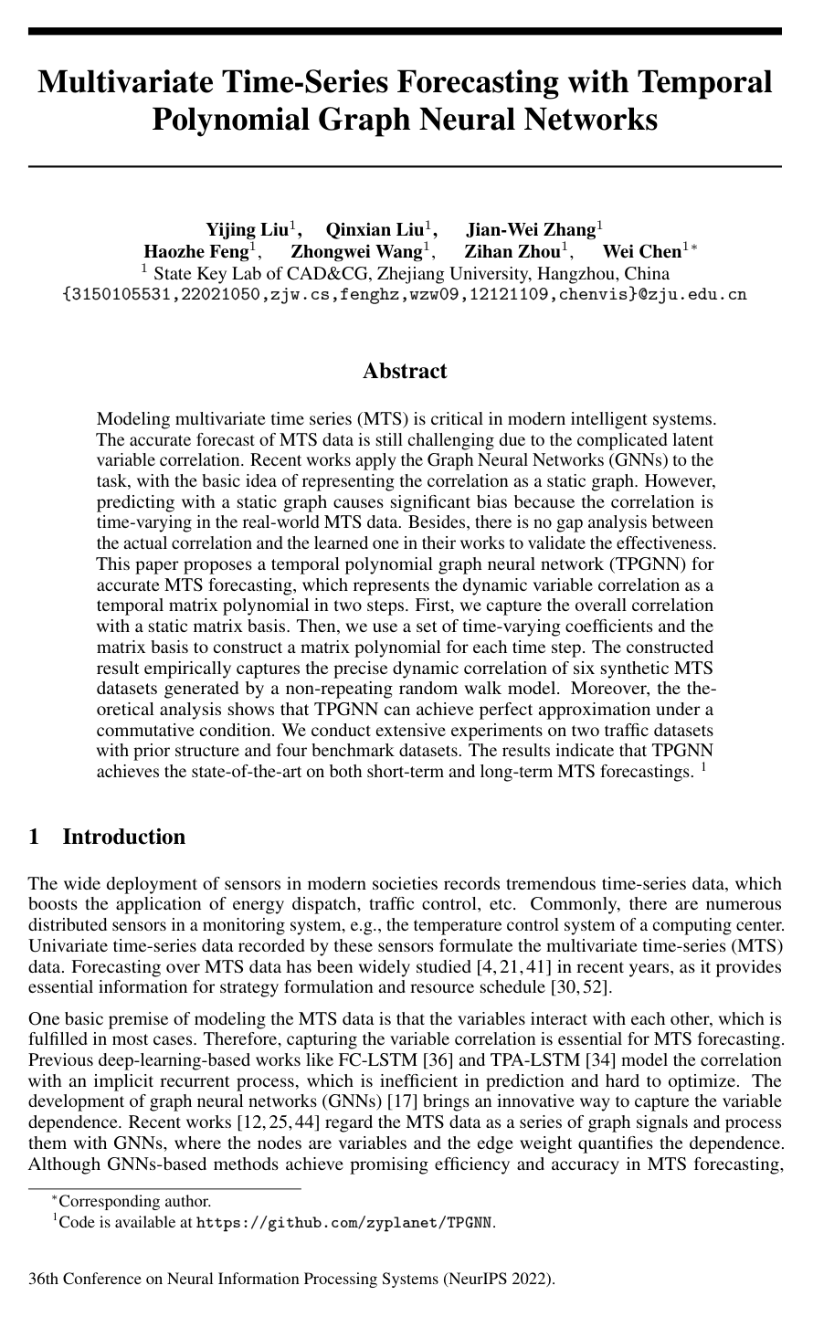
Modeling multivariate time series (MTS) is critical in modern intelligent systems. The accurate forecast of MTS data is still challenging due to the complicated latent variable correlation. Recent works apply the Graph Neural Networks (GNNs) to the task, with the basic idea of representing the correlation as a static graph. However, predicting with a static graph causes significant bias because the correlation is time-varying in the real-world MTS data. Besides, there is no gap analysis between the actual correlation and the learned one in their works to validate the effectiveness. This paper proposes a temporal polynomial graph neural network (TPGNN) for accurate MTS forecasting, which represents the dynamic variable correlation as a temporal matrix polynomial in two steps. First, we capture the overall correlation with a static matrix basis. Then, we use a set of time-varying coefficients and the matrix basis to construct a matrix polynomial for each time step. The constructed result empirically captures the precise dynamic correlation of six synthetic MTS datasets generated by a non-repeating random walk model. Moreover, the theoretical analysis shows that TPGNN can achieve perfect approximation under a commutative condition. We conduct extensive experiments on two traffic datasets with prior structure and four benchmark datasets. The results indicate that TPGNN achieves the state-of-the-art on both short-term and long-term MTS forecastings. 1

Topics

graph embeddings graph neural networks network architecture recurrent neural networks

Keywords

Temporal Polynomial Graph Neural Networks multivariate time-series forecasting Graph WaveNet spatio-temporal graph neural networks traffic forecasting matrix polynomials graph filters time-varying coefficients temporal attention layer

1 Introduction
2 Related Works
3 The Framework of TPGNN
3.1 Problem Definition
3.2 Represent the Correlation as a Temporal Matrix Polynomial
3.3 Inference Pipeline
4 Theoretical Properties of TPGNN
5 Experiments
5.1 Experimental Setup
5.2 Main Results
5.3 Ablation Experiments
5.4 Study of the Graph Structure Approximation Gap
6 Conclusion
7 Acknowledgment
References

Knowls

Knowl 1 — Temporal polynomial representation of dynamic variable dependence
model/method
TPGNN treats an $N$ -variable multivariate time series as a time-indexed graph signal $\mathcal{G}^{(t)}=(V,E^{(t)},X^{(t)},W^{(t)})$ , where $X^{(t)}\in\mathbb{R}^{N\times 1}$ is the variable state and $W^{(t)}\in\mathbb{R}^{N\times N}$ is a time-varying weighted adjacency matrix. Given $T$ historical graph signals, the forecasting task is to predict the next $T_0$ signals:
$\big(\mathcal{G}^{(t)},\ldots,\mathcal{G}^{(t+T-1)}\big)\mapsto\big(X^{(t+T)},\ldots,X^{(t+T+T_0-1)}\big).$
TPGNN represents the dynamic dependence at time $t$ with a polynomial of one shared adjacency basis $A\in\mathbb{R}^{N\times N}$ :
$W^{(t)}=\sum_{k=0}^{K}a_k^{(t)}A^k,$
where $K$ is the polynomial order, $A^k$ is the $k$ -step matrix power, and $a_k^{(t)}$ is a coefficient that varies with time. Thus, the graph changes over time through the coefficients rather than through a separately learned adjacency matrix at every time step.
Knowl 2 — Self-adaptive adjacency basis with optional prior structure
model/method
TPGNN learns a shared adjacency basis from variable embeddings. If $E\in\mathbb{R}^{N\times c}$ contains $c$ -dimensional embeddings for the $N$ variables, the data-driven basis is
$A=\operatorname{SoftMax}\!\left(\operatorname{ReLU}(EE^{\mathsf T})\right),$
where the ReLU removes negative similarities and SoftMax normalizes the resulting similarities. For datasets with a known prior adjacency matrix $W_{\mathrm{prior}}\in\mathbb{R}^{N\times N}$ , TPGNN additionally computes
$L=D^{-1/2}(I+W_{\mathrm{prior}})D^{-1/2},$
where $I$ is the $N\times N$ identity matrix and $D$ is the degree matrix of $I+W_{\mathrm{prior}}$ , and uses
$A=\operatorname{SoftMax}\!\left(\operatorname{ReLU}(EE^{\mathsf T})\right)+L.$
The learned component allows the forecasting objective to discover dependencies that are absent from the supplied physical or spatial structure.
Knowl 3 — Cyclic timestamp coefficients and window-level averaging
model/method
To generate time-varying polynomial coefficients without learning an independent parameter vector for every possible time index, TPGNN uses periodic timestamp embeddings. Let $T_p$ be the assumed cycle length, let $e_{\mathrm{ts}}^{(r)}\in\mathbb{R}^{D_e}$ for $r=1,\ldots,T_p$ be learnable cyclic timestamp embeddings, and let $W_c\in\mathbb{R}^{D_e\times(K+1)}$ be a coefficient matrix. The coefficient vector for time $s$ is obtained from the embedding indexed by $s\bmod T_p$ :
$a^{(s)}=e_{\mathrm{ts}}^{(s\bmod T_p)}W_c\in\mathbb{R}^{K+1}.$
For an input window beginning at time $t$ and containing $T$ signals, TPGNN computes the coefficient vectors for all $T$ timestamps and combines them with a learned averaging vector $W_a\in\mathbb{R}^{T\times 1}$ :
$\bar a=(\bar a_0,\ldots,\bar a_K)=\big(a^{(t)},a^{(t+1)},\ldots,a^{(t+T-1)}\big)W_a.$
The resulting $\bar a$ defines one polynomial for the whole input window. Because matrix polynomials are linear in their coefficients, this is equivalent to averaging the corresponding time-specific polynomial outputs, while avoiding the cost of propagating all $T$ polynomials separately.
Knowl 4 — TPG propagation layer
model/method
Given an embedded signal matrix $X^{(t)}\in\mathbb{R}^{N\times D_e}$ , the TPG module produces a hidden representation $Z^{(t)}\in\mathbb{R}^{N\times D_e}$ using the averaged temporal coefficients $\bar a_k$ :
$Z^{(t)}=\sum_{k=0}^{K}\bar a_k A^k X^{(t)}\frac{W_k}{\lVert W_k\rVert_F},$
where $W_k\in\mathbb{R}^{D_e\times D_e}$ is a separately learned feature-transformation matrix for polynomial order $k$ , and $\lVert\cdot\rVert_F$ is the Frobenius norm. The $K+1$ distinct matrices $W_k$ increase representation diversity across graph orders. Dividing each matrix by its Frobenius norm decouples the magnitude of the feature transformation from $\bar a_k$ , so the temporal polynomial coefficients control the relative contribution of the graph-order terms.
Knowl 5 — Autoregressive encoder-decoder forecasting pipeline
model/method
TPGNN first maps historical scalar signals into $D_e$ -dimensional embeddings. An encoder applies the TPG propagation layer and a Transformer-style temporal self-attention layer to the $T$ historical signals, producing encodings $Z^{(t:t+T-1)}\in\mathbb{R}^{T\times N\times D_e}$ . A decoder uses these encodings to forecast autoregressively. For the first forecast, a learnable beginning-of-sequence embedding $E_{\mathrm{BOS}}\in\mathbb{R}^{N\times D_e}$ queries the encoder output:
$E_X^{(t+T)}=\operatorname{Decoder}(E_{\mathrm{BOS}},Z^{(t:t+T-1)}),\qquad \widetilde X^{(t+T)}=E_X^{(t+T)}W_{\mathrm{pred}},$
where $W_{\mathrm{pred}}\in\mathbb{R}^{D_e\times 1}$ maps decoder embeddings to the $N$ predicted variable values. For later forecasts, the decoder queries the same encoder output using the latest $L_{\max}$ decoder outputs. After $k$ predictions, the next decoder state and prediction are
$E_X^{(t+T+k)}=\operatorname{Decoder}\!\left(E_X^{(t+T+k-L_{\max})},\ldots,E_X^{(t+T+k-1)},Z^{(t:t+T-1)}\right),$ $\widetilde X^{(t+T+k)}=E_X^{(t+T+k)}W_{\mathrm{pred}}.$
This process continues until all $T_0$ future signals have been generated, allowing the decoder to use its recent predictions as context for long-horizon forecasting.
Knowl 6 — Approximation guarantee under commuting graph structure
theoretical result
Let $G^{(1)},\ldots,G^{(T)}\in\mathbb{R}^{N\times N}$ be the symmetric normalized Laplacians of the optimal undirected graph structures at $T$ time steps, and let $A\in\mathbb{R}^{N\times N}$ be TPGNN's initial adjacency basis. Suppose that all $G^{(t)}$ and $A$ are symmetric, every pair of target matrices commutes, $G^{(i)}G^{(j)}=G^{(j)}G^{(i)}$ for all $i,j$ , $A$ has $N$ distinct singular values, and the polynomial order $K$ is sufficiently large. If
$e_{1:T}=\frac{1}{T}\sum_{t=1}^{T}\lVert W^{(t)}-G^{(t)}\rVert_F^2$
is the mean squared Frobenius approximation error, then TPGNN satisfies
$(1-\lambda_{\max})\,\mathbb{E}_t\!\left[\lVert G^{(t)}\rVert_F^2\right] \leq e_{1:T}\leq (1-\lambda_{\min})\,\mathbb{E}_t\!\left[\lVert G^{(t)}\rVert_F^2\right],$
where $\lambda_{\min},\lambda_{\max}\in[0,1]$ are the minimum and maximum eigenvalues of the constant matrix appearing in the polynomial approximation bound, and $\mathbb{E}_t[\lVert G^{(t)}\rVert_F^2]=T^{-1}\sum_{t=1}^{T}\lVert G^{(t)}\rVert_F^2$ . When $A$ commutes with every $G^{(t)}$ , the theorem gives $\lambda_{\min}=\lambda_{\max}=1$ and therefore $e_{1:T}=0$ : under this condition and sufficiently high order, TPGNN can represent the target dynamic graph sequence perfectly.
Knowl 7 — Synthetic dynamic-dependence benchmark and approximation results
empirical result
The paper evaluates dependence approximation on six synthetic multivariate time series with known dynamic graphs. At each time $t$ , the signal $X^{(t)}\in\mathbb{R}^{N\times1}$ is generated by a non-repeating random-walk process,
$X^{(t)}\sim\mathcal{N}\!\left(W^{(t-1)}X^{(t-1)},\sigma\right),$
where $W^{(t)}$ is a time-varying weighted adjacency matrix, $\sigma$ controls the Gaussian variation, and $X^{(0)}$ is sampled from a discrete uniform distribution. The dynamic graph cycles through $N_w$ Laplacian matrices $G^{(1)},\ldots,G^{(N_w)}$ over period $T_p$ , with each matrix used for an equal interval; $N_w=1,\ldots,6$ controls dependence complexity. The experiments used $T_p=120$ , $\sigma=0.001$ , sequence length $2400$ , a 7:1:2 train/validation/test split, polynomial order $K=2$ , and five repetitions. The graph approximation metric was
$\mathrm{MFE}=\frac{1}{TN^2}\sum_{t=0}^{T-1}\left\lVert W^{(t)}-\widetilde W^{(t)}\right\rVert_F,$
where $\widetilde W^{(t)}$ is the learned adjacency matrix. TPGNN was compared with Graph WaveNet, MTGNN, GPR-GNN, and self-attention-based graph learning.

The average results across the six synthetic datasets were:
Could not parse LaTeX table
TPGNN had the lowest average MFE, MAE, and RMSE and reduced MFE by 23.41% relative to the strongest competing method on average. Its MFE decreased as $N_w$ increased, whereas the competing methods generally became less accurate. The ordering of methods by MFE matched their ordering by forecasting error, supporting the paper's claim that more precise dynamic-dependence recovery improves MTS forecasting. Increasing the polynomial order from $K=1$ to $K=4$ substantially increased approximation variance, and $K=4$ produced the largest MFE; the paper therefore finds that high-order polynomials reduce precision and robustness in this MTS setting.
Knowl 8 — Forecasting performance on six real-world datasets
data/table
TPGNN was evaluated on four single-step benchmark datasets—Solar-Energy, Traffic, Electricity, and Exchange-Rate—and two multi-step traffic datasets—PEMS-BAY and PEMS-D7. The first four datasets used input length 168 and forecast horizons 3, 6, 12, and 24; PEMS-BAY and PEMS-D7 used 12 historical steps and forecast horizons 3, 6, and 12. Data were split 7:1:2 into training, validation, and test sets. Lower RSE, MAE, MAPE, and RMSE are better, while higher CORR is better.

The reported TPGNN scores were:
Could not parse LaTeX table
Could not parse LaTeX table
Against recurrent, convolutional, graph-neural, and Transformer baselines, TPGNN achieved the reported state of the art on five of the six datasets and was not the best method on Exchange-Rate, which the paper attributes partly to its small sample size. On Solar-Energy, TPGNN reduced RSE by 1.61% and 18.08% at horizons 12 and 24 and increased CORR by 1.47% and 6.93% at those horizons. On Traffic it improved CORR by 2.21% on average across the four horizons, and on Electricity it reduced RSE by 15.82% on average. For the multi-step traffic task, it reduced PEMS-BAY MAPE by 5.47% on average and reduced PEMS-D7 MAE and MAPE by 8.04% and 6.61% on average.
Knowl 9 — Component ablation on long-horizon traffic forecasting
data/table
Ablation experiments on PEMS-D7 used a 12-step forecast horizon and five repetitions; each entry is the mean $\pm$ standard deviation. The variants remove the temporal polynomial graph module, time-varying coefficients, window-level coefficient averaging, normalization of $W_k$ , or the separate order-specific matrices.
Could not parse LaTeX table
Replacing the TPG module with the supplied prior graph caused the largest degradation: MAE, MAPE, and RMSE worsened by 13.13%, 13.94%, and 12.23%, respectively. Replacing time-varying coefficients with static coefficients worsened long-term accuracy by 7.04% on average, demonstrating the importance of dynamic dependence. Removing the window-level averaging or the order-specific matrices produced larger variance, indicating that both mechanisms improve robustness. Removing coefficient normalization had a smaller effect, but still degraded all three metrics.
Knowl 10 — Real-world evidence of learned dynamic correlations
empirical result
A case study on PEMS-D7 examined nodes 60, 93, and 218, which are independent in the supplied physical prior structure but highly correlated in the dependence learned by TPGNN. The three sensors lie on the same road, providing a plausible physical basis for the newly discovered relationships. The learned correlation between nodes 93 and 218 remains relatively stable over time, whereas the correlation between nodes 60 and 218 increases in the evening. The paper associates this difference with the branch road between nodes 218 and 60. This example demonstrates that the data-driven component of TPGNN can recover useful relationships that are not encoded by a static sensor-distance graph and can represent different temporal correlation patterns for different variable pairs.
Knowl 11 — Stated limitations of TPGNN
limitation
The dependence learned by TPGNN is a correlation structure rather than a strict causal graph, so some learned relationships may be unreliable and may reduce robustness. In addition, rare real-world events such as weather disasters can substantially disrupt multivariate time-series dynamics and impair forecasting accuracy. The paper identifies causal learning and transfer learning as directions for addressing these limitations.

Coverage note — Secondary implementation details, hyperparameter-search settings, baseline descriptions, and appendix-only analyses were omitted because they do not materially change the proposed model, theory, or main empirical conclusions.

References

1.ADHIKARI, R., AND AGRAWAL, R. K. A combination of artificial neural network and random walk models for financial time series forecasting. Neural Computing and Applications 24 (2013), 1441–1449.
2.ASUNCION, A., AND NEWMAN, D. J. Uci machine learning repository. [EB/OL], 2007. http://www.ics.uci.edu/~mlearn/MLRepository.html.
3.CA.GOV. Pems. [EB/OL], 2010. https://pems.dot.ca.gov/.
4.CAO, D., WANG, Y., DUAN, J., ZHANG, C., ZHU, X., HUANG, C., TONG, Y., XU, B., BAI, J., TONG, J., ET AL. Spectral temporal graph neural network for multivariate time-series forecasting. arXiv preprint arXiv:2103.07719 (2021).
5.CHIEN, E., PENG, J., LI, P., AND MILENKOVIC, O. Adaptive universal generalized pagerank graph neural network. arXiv: Learning (2021).
6.DEFFERRARD, M., BRESSON, X., AND VANDERGHEYNST, P. Convolutional neural networks on graphs with fast localized spectral filtering. In NIPS (2016).
7.DENTON, A. M. Kernel-density-based clustering of time series subsequences using a continuous random-walk noise model. Fifth IEEE International Conference on Data Mining (ICDM’05) (2005), 8 pp.–.
8.DLOTKO, P., QIU, W., AND RUDKIN, S. Cyclicality, periodicity and the topology of time series. ArXiv abs/1905.12118 (2019).
9.FENG, H., YOU, Z., CHEN, M., ZHANG, T., ZHU, M., WU, F., WU, C., AND CHEN, W. KD3A: unsupervised multi-source decentralized domain adaptation via knowledge distillation. In Proceedings of the 38th International Conference on Machine Learning, ICML 2021, 18-24 July 2021, Virtual Event (2021), M. Meila and T. Zhang, Eds., vol. 139 of Proceedings of Machine Learning Research, PMLR, pp. 3274–3283.
10.FRIGOLA, R. Bayesian time series learning with Gaussian processes. PhD thesis, University of Cambridge, 2015.
11.GAMA, F., ISUFI, E., LEUS, G., AND RIBEIRO, A. Graphs, convolutions, and neural networks: From graph filters to graph neural networks. IEEE Signal Processing Magazine 37 (2020), 128–138.
12.GUO, S., LIN, Y., FENG, N., SONG, C., AND WAN, H. Attention based spatial-temporal graph convolutional networks for traffic flow forecasting. In Proceedings of the AAAI Conference on Artificial Intelligence (2019), vol. 33, pp. 922–929.
13.HADOU, S., KANATSOULIS, C. I., AND RIBEIRO, A. Space-time graph neural networks. ArXiv abs/2110.02880 (2021).
14.HAMILTON, W. L., YING, R., AND LESKOVEC, J. Inductive representation learning on large graphs. arXiv preprint arXiv:1706.02216 (2017).
15.ISUFI, E., LOUKAS, A., PERRAUDIN, N., AND LEUS, G. Forecasting time series with varma recursions on graphs. IEEE Transactions on Signal Processing 67 (2019), 4870–4885.
16.ISUFI, E., AND MAZZOLA, G. Graph-time convolutional neural networks. 2021 IEEE Data Science and Learning Workshop (DSLW) (2021), 1–6.
17.KIPF, T. N., AND WELLING, M. Semi-supervised classification with graph convolutional networks. arXiv preprint arXiv:1609.02907 (2016).
18.KLICPERA, J., BOJCHEVSKI, A., AND GÜNNEMANN, S. Predict then propagate: Graph neural networks meet personalized pagerank. In ICLR (2019).
19.LAI, G., CHANG, W.-C., YANG, Y., AND LIU, H. Modeling long- and short-term temporal patterns with deep neural networks. The 41st International ACM SIGIR Conference on Research & Development in Information Retrieval (2018).
20.LAI, G., CHANG, W.-C., YANG, Y., AND LIU, H. Modeling long-and short-term temporal patterns with deep neural networks. In The 41st International ACM SIGIR Conference on Research & Development in Information Retrieval (2018), pp. 95–104.
21.LEE, W. K. Partial correlation-based attention for multivariate time series forecasting. In Proceedings of the AAAI Conference on Artificial Intelligence (2020), vol. 34, pp. 13720–13721.
22.LI, Y., YU, R., SHAHABI, C., AND LIU, Y. Diffusion convolutional recurrent neural network: Data-driven traffic forecasting. arXiv preprint arXiv:1707.01926 (2017).
23.LI, Y., YU, R., SHAHABI, C., AND LIU, Y. Diffusion convolutional recurrent neural network: Data-driven traffic forecasting. arXiv: Learning (2018).
24.LIANG, X. S. Normalized multivariate time series causality analysis and causal graph reconstruction. Entropy 23 (2021).
25.MENGZHANG, L., AND ZHANXING, Z. Spatial-temporal fusion graph neural networks for traffic flow forecasting. arXiv preprint arXiv:2012.09641 (2020).
26.NATALI, A., ISUFI, E., COUTIÑO, M., AND LEUS, G. Learning time-varying graphs from online data. IEEE Open Journal of Signal Processing 3 (2022), 212–228.
27.ORESHKIN, B. N., AMINI, A., COYLE, L., AND COATES, M. J. Fc-gaga: Fully connected gated graph architecture for spatio-temporal traffic forecasting. ArXiv abs/2007.15531 (2021).
28.PAN, S. J., AND YANG, Q. A survey on transfer learning. IEEE Transactions on Knowledge and Data Engineering 22 (2010), 1345–1359.
29.PUECH, T., BOUSSARD, M., D’AMATO, A., AND MILLERAND, G. A fully automated periodicity detection in time series. In AALTD@PKDD/ECML (2019).
30.QING, L., YONGQIN, T., YONG-GUO, H., AND QINGMING, Z. The forecast and the optimization control of the complex traffic flow based on the hybrid immune intelligent algorithm. The Open Electrical & Electronic Engineering Journal 8 (2014), 245–251.
31.ROBERTS, S., OSBORNE, M., EBDEN, M., REECE, S., GIBSON, N., AND AIGRAIN, S. Gaussian processes for time-series modelling. Philosophical Transactions of the Royal Society A: Mathematical, Physical and Engineering Sciences 371, 1984 (2013), 20110550.
32.SARIA, S., DUCHI, A., AND KOLLER, D. Discovering deformable motifs in continuous time series data. In IJCAI (2011).
33.SHAFIPOUR, R., SEGARRA, S., MARQUES, A. G., AND MATEOS, G. Identifying the topology of undirected networks from diffused non-stationary graph signals. IEEE Open Journal of Signal Processing 2 (2021), 171–189.
34.SHIH, S.-Y., SUN, F.-K., AND LEE, H.-Y. Temporal pattern attention for multivariate time series forecasting. Machine Learning 108, 8 (2019), 1421–1441.
35.SONG, C., LIN, Y., GUO, S., AND WAN, H. Spatial-temporal synchronous graph convolutional networks: A new framework for spatial-temporal network data forecasting. In Proceedings of the AAAI Conference on Artificial Intelligence (2020), vol. 34, pp. 914–921.
36.SUTSKEVER, I., VINYALS, O., AND LE, Q. V. Sequence to sequence learning with neural networks. arXiv preprint arXiv:1409.3215 (2014).
37.VASWANI, A., SHAZEER, N., PARMAR, N., USZKOREIT, J., JONES, L., GOMEZ, A. N., KAISER, L., AND POLOSUKHIN, I. Attention is all you need. arXiv preprint arXiv:1706.03762 (2017).
38.WEN, T., AND KEYES, R. Time series anomaly detection using convolutional neural networks and transfer learning. ArXiv abs/1905.13628 (2019).
39.WU, C.-H., HO, J.-M., AND LEE, D.-T. Travel-time prediction with support vector regression. IEEE transactions on intelligent transportation systems 5, 4 (2004), 276–281.
40.WU, F., ZHANG, T., DE SOUZA, A. H., FIFTY, C., YU, T., AND WEINBERGER, K. Q. Simplifying graph convolutional networks. ArXiv abs/1902.07153 (2019).
41.WU, Z., PAN, S., LONG, G., JIANG, J., CHANG, X., AND ZHANG, C. Connecting the dots: Multivariate time series forecasting with graph neural networks. In Proceedings of the 26th ACM SIGKDD International Conference on Knowledge Discovery & Data Mining (2020), pp. 753–763.
42.WU, Z., PAN, S., LONG, G., JIANG, J., AND ZHANG, C. Graph wavenet for deep spatial-temporal graph modeling. arXiv preprint arXiv:1906.00121 (2019).
43.XU, M., DAI, W., LIU, C., GAO, X., LIN, W., QI, G.-J., AND XIONG, H. Spatial-temporal transformer networks for traffic flow forecasting. ArXiv abs/2001.02908 (2020).
44.YU, B., YIN, H., AND ZHU, Z. Spatio-temporal graph convolutional networks: A deep learning framework for traffic forecasting. arXiv preprint arXiv:1709.04875 (2017).
45.ZAMAN, B., RAMOS, L. M. L., ROMERO, D., AND BEFERULL-LOZANO, B. Online topology identification from vector autoregressive time series. IEEE Transactions on Signal Processing 69 (2021), 210–225.
46.ZERVEAS, G., JAYARAMAN, S., PATEL, D., BHAMIDIPATY, A., AND EICKHOFF, C. A transformer-based framework for multivariate time series representation learning. Proceedings of the 27th ACM SIGKDD Conference on Knowledge Discovery & Data Mining (2021).
47.ZHANG, G. P. Time series forecasting using a hybrid arima and neural network model. Neurocomputing 50 (2003), 159–175.
48.ZHANG, J.-W., SUN, Y., YANG, Y., AND CHEN, W. Feature-Proxy Transformer for Few-Shot Segmentation. In NeurIPS (2022).
49.ZHANG, Q., CHANG, J., MENG, G., XIANG, S., AND PAN, C. Spatio-temporal graph structure learning for traffic forecasting. In Proceedings of the AAAI Conference on Artificial Intelligence (2020), vol. 34, pp. 1177–1185.
50.ZHENG, C., FAN, X., WANG, C., AND QI, J. Gman: A graph multi-attention network for traffic prediction. In Proceedings of the AAAI Conference on Artificial Intelligence (2020), vol. 34, pp. 1234–1241.
51.ZHOU, H., ZHANG, S., PENG, J., ZHANG, S., LI, J., XIONG, H., AND ZHANG, W. Informer: Beyond efficient transformer for long sequence time-series forecasting. In AAAI (2021).
52.ZHOU, X., YAN, H., ZHANG, H., AND PENG, C. Model predictive control with feedback correction for optimal energy dispatch of a networked microgrid. Transactions of the Institute of Measurement and Control 41 (2019), 1540 – 1552.

Citation

MLA

Liu, Y., et al. “Multivariate Time-Series Forecasting with Temporal Polynomial Graph Neural Networks”. Advances in Neural Information Processing Systems, vol. 35, 2022, pp. 19414–26, https://proceedings.neurips.cc/paper_files/paper/2022/file/7b102c908e9404dd040599c65db4ce3e-Paper-Conference.pdf.

APA

Liu, Y., Liu, Q., Zhang, J.-W., Feng, H., Wang, Z., Zhou, Z., & Chen, W. (2022). Multivariate Time-Series Forecasting with Temporal Polynomial Graph Neural Networks. Advances in Neural Information Processing Systems, 35, 19414–19426. https://proceedings.neurips.cc/paper_files/paper/2022/file/7b102c908e9404dd040599c65db4ce3e-Paper-Conference.pdf

Chicago

Liu, Y., Q. Liu, J.-W. Zhang, et al. 2022. “Multivariate Time-Series Forecasting with Temporal Polynomial Graph Neural Networks”. Advances in Neural Information Processing Systems 35: 19414–26. https://proceedings.neurips.cc/paper_files/paper/2022/file/7b102c908e9404dd040599c65db4ce3e-Paper-Conference.pdf.

Harvard

Liu, Y. et al. (2022) “Multivariate Time-Series Forecasting with Temporal Polynomial Graph Neural Networks”, Advances in Neural Information Processing Systems. Curran Associates, Inc., pp. 19414–19426. Available at: https://proceedings.neurips.cc/paper_files/paper/2022/file/7b102c908e9404dd040599c65db4ce3e-Paper-Conference.pdf.

Vancouver

1. Liu Y, Liu Q, Zhang J-W, Feng H, Wang Z, Zhou Z, Chen W (2022) Multivariate Time-Series Forecasting with Temporal Polynomial Graph Neural Networks. In: Advances in Neural Information Processing Systems. Curran Associates, Inc., pp 19414–19426

BibTeX

@inproceedings{liu2022multivariate,
  title = {Multivariate Time-Series Forecasting with Temporal Polynomial Graph Neural Networks},
  author = {Liu, Yijing and Liu, Qinxian and Zhang, Jian-Wei and Feng, Haozhe and Wang, Zhongwei and Zhou, Zihan and Chen, Wei},
  year = {2022},
  booktitle = {Advances in Neural Information Processing Systems},
  publisher = {Curran Associates, Inc.},
  volume = {35},
  pages = {19414-19426},
  url = {https://proceedings.neurips.cc/paper_files/paper/2022/file/7b102c908e9404dd040599c65db4ce3e-Paper-Conference.pdf}
}

Metadata:DOI registry

Source Code

This paper has an official code repository available. Click below to access the source code.

View Repository

Access the Paper

This paper is available from its original source. Click below to access the PDF.

Open PDF

License: Authors

Multivariate Time-Series Forecasting with Temporal Polynomial Graph Neural Networks

Abstract

Topics

Keywords

Table of Contents

Knowls

Knowl 1 — Temporal polynomial representation of dynamic variable dependence

Knowl 2 — Self-adaptive adjacency basis with optional prior structure

Knowl 3 — Cyclic timestamp coefficients and window-level averaging

Knowl 4 — TPG propagation layer

Knowl 5 — Autoregressive encoder-decoder forecasting pipeline

Knowl 6 — Approximation guarantee under commuting graph structure

Knowl 7 — Synthetic dynamic-dependence benchmark and approximation results

Knowl 8 — Forecasting performance on six real-world datasets

Knowl 9 — Component ablation on long-horizon traffic forecasting

Knowl 10 — Real-world evidence of learned dynamic correlations

Knowl 11 — Stated limitations of TPGNN

References

Citation

BibTeX

Source Code

Access the Paper