Learning Discriminative Model Prediction for Tracking

Goutam BhatMartin DanelljanLuc Van GoolRadu Timofte

article2019ICCV1,367 citations

Develops an end-to-end visual tracking architecture that integrates online discriminative target model prediction using an efficient optimization process to achieve state-of-the-art accuracy across six benchmarks at real-time speeds exceeding 40 frames per second.

Listen

Visual object tracking—the task of estimating an arbitrary target's location across video frames given only its initial bounding box—is essential for autonomous systems, robotics, and video analytics. A core challenge is learning a target appearance model during runtime that accurately distinguishes the object from background clutter and distractors. Existing approaches face a fundamental trade-off: end-to-end trainable Siamese networks are fast but ignore background context during inference, leading to tracking failures, while discriminative online learning methods utilize background context but rely on complex, hand-crafted optimization procedures that prevent end-to-end training.

The article introduces and evaluates a novel, end-to-end trainable discriminative model prediction architecture (named DiMP) for visual tracking. The objective is to demonstrate that integrating an iterative, background-aware optimization procedure directly into a deep neural network yields superior target-background discriminability, robust online model updates, and state-of-the-art tracking performance at real-time speeds.

To evaluate this approach, the researchers designed an optimization module based on the steepest descent method that computes optimal step lengths per iteration, allowing the model to converge in only a few steps. They also integrated a model initialization module and parameterized the discriminative learning loss so its internal components (such as target masks and spatial weights) could be learned directly from data. The entire network was trained offline across large-scale video datasets (TrackingNet, LaSOT, GOT10k, and COCO) and evaluated across seven challenging benchmark datasets: VOT2018, LaSOT, TrackingNet, GOT10k, Need for Speed (NFS), OTB-100, and UAV123.

The experimental findings show that the proposed framework sets a new state of the art across six of the seven benchmarks while operating at over 40 frames per second (FPS). On the VOT2018 benchmark, the ResNet-50 variant achieved an Expected Average Overlap (EAO) of 0.440, outperforming the leading Siamese baseline (SiamRPN++) by 6.3% while reducing the tracking failure rate by 34%. On the GOT10k benchmark, which strictly tests generalization to unseen object classes without external training data, the tracker led the field with an Average Overlap score of 61.1%. Component analysis confirmed that the steepest descent optimizer outperformed standard gradient descent by 2.2% in Area Under the Curve (AUC), and incorporating background-aware online updates yielded a 2.0% AUC improvement over static or naively averaged models. Furthermore, tests on training data scaling revealed high sample efficiency, suffering only a 1.5% AUC drop when trained on just 10% of the video training data.

These results demonstrate that online discriminative learning can be fully unified with end-to-end deep learning architectures without sacrificing inference speed. For decision-makers and engineering leads, this architecture significantly lowers operational risk in automated vision systems by reducing target loss in complex, cluttered scenes while maintaining the low computational overhead necessary for deployment on real-time hardware.

Organizations developing or upgrading vision pipelines should consider adopting this discriminative prediction architecture over pure Siamese or static template-matching baselines, particularly for long-duration tracking and cluttered environments. As next steps, teams should validate performance on target edge-device hardware and evaluate domain-specific fine-tuning if target operating environments differ significantly from general video benchmarks.

Confidence in these findings is high given the breadth of evaluation across multiple standard benchmarks and extensive ablation experiments. However, practitioners should note that benchmark performance relies on high-end desktop GPU hardware (e.g., Nvidia GTX 1080), meaning embedded platforms with constrained compute may require lighter backbone networks to sustain the reported 40+ FPS frame rates.

ETH Zurich appearance models inference object appearance discriminative model prediction visual object tracking target model predictor

arXiv: 1904.07220

Paper: Fully-Convolutional Siamese Networks for Object Tracking, Luca Bertinetto et al. (2016). Introduces the foundational fully-convolutional Siamese tracking framework (SiamFC) whose lack of online target-background discriminability directly motivates the end-to-end model prediction architecture.
Paper: End-to-End Representation Learning for Correlation Filter Based Tracking, Jack Valmadre et al. (2017). Pioneers end-to-end differentiable correlation filter learning within Siamese networks (CFNet), establishing the concept of embedding an optimization objective directly inside the neural architecture.
Paper: ECO: Efficient Convolution Operators for Tracking, Martin Danelljan et al. (2017). Provides the advanced discriminative correlation filter formulation and optimization strategies that serve as a direct conceptual predecessor to learning online discriminative model prediction.
Paper: Beyond Correlation Filters: Learning Continuous Convolution Operators for Visual Tracking, Martin Danelljan et al. (2016). Formulates continuous convolution operators for tracking (C-COT), which forms the continuous discriminative learning baseline that subsequent end-to-end optimization tracking methods refine.
Paper: SiamRPN++: Evolution of Siamese Visual Tracking With Very Deep Networks, Bo Li et al. (2018). Demonstrates modern deep Siamese tracking using ResNet backbones and region proposal networks (SiamRPN++), representing the state-of-the-art template-matching paradigm improved upon by the source.
Paper: Learning Spatially Regularized Correlation Filters for Visual Tracking, Martin Danelljan et al. (2015). Develops spatially regularized correlation filters (SRDCF) to mitigate background boundary effects, establishing key mathematical loss formulations for discriminative tracking.
Paper: Learning Multi-domain Convolutional Neural Networks for Visual Tracking, Hyeonseob Nam et al. (2016). Establishes multi-domain online CNN fine-tuning for tracking (MDNet), highlighting both the power and computational overhead of online target modeling.
Paper: LaSOT: A High-Quality Benchmark for Large-Scale Single Object Tracking, Heng Fan et al. (2018). Introduces the LaSOT benchmark used extensively to evaluate and demonstrate the long-term discriminative capabilities of the proposed architecture.

Paper: Transformer Tracking, Xin Chen et al. (2021). Advances visual object tracking beyond explicit optimization-based model prediction by utilizing Transformer attention mechanisms for global template-search feature fusion.

Cover for Learning Discriminative Model Prediction for Tracking

Abstract

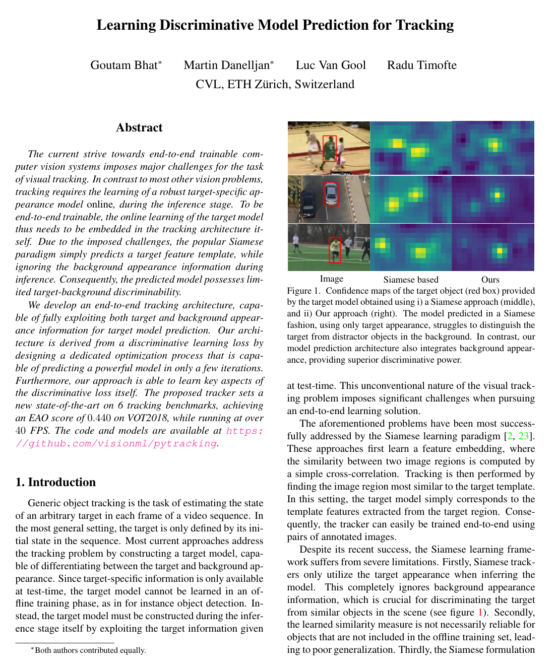
The current strive towards end-to-end trainable computer vision systems imposes major challenges for the task of visual tracking. In contrast to most other vision problems, tracking requires the learning of a robust target-specific appearance model online, during the inference stage. To be end-to-end trainable, the online learning of the target model thus needs to be embedded in the tracking architecture itself. Due to the imposed challenges, the popular Siamese paradigm simply predicts a target feature template, while ignoring the background appearance information during inference. Consequently, the predicted model possesses limited target-background discriminability.

We develop an end-to-end tracking architecture, capable of fully exploiting both target and background appearance information for target model prediction. Our architecture is derived from a discriminative learning loss by designing a dedicated optimization process that is capable of predicting a powerful model in only a few iterations. Furthermore, our approach is able to learn key aspects of the discriminative loss itself. The proposed tracker sets a new state-of-the-art on 6 tracking benchmarks, achieving an EAO score of 0.440 on VOT2018, while running at over 40 FPS. The code and models are available at this https URL.

Topics

appearance models inference object appearance online learning optimization target model vision systems

Keywords

discriminative model prediction visual object tracking target model predictor discriminative learning loss online tracking Siamese trackers box estimation correlation filters least-squares regression

1 Introduction
2 Related Work
3 Method
3.1 Discriminative Learning Loss
3.2 Optimization-Based Architecture
3.3 Initial Filter Prediction
3.4 Learning the Discriminative Learning Loss
3.5 Bounding Box Estimation
3.6 Offline Training
3.7 Online Tracking
4 Experiments
4.1 Analysis of our Approach
4.2 State-of-the-art Comparison
5 Conclusions
References
S1 Closed-Form Expression for ∇L\nabla L
S2 Calculation of hh in Algorithm
S3 Detailed Results on VOT2018
S4 Detailed Results on LaSOT
S5 Detailed Results on NFS, OTB-100, and UAV123
S6 Impact of Training Data
S7 Visualizations of learned ycy_{c}, mcm_{c}, and vcv_{c}

Knowls

Knowl 1 — Discriminative Model Prediction (DiMP) Tracking Architecture
model/method
The Discriminative Model Prediction (DiMP) tracking architecture is an end-to-end trainable visual tracking framework consisting of two main functional branches built upon a shared deep convolutional backbone feature extractor $F$ (such as ResNet-18 or ResNet-50):
1. Target Classification Branch: Tasked with discriminating the target object from background distractors. Deep feature maps extracted from the backbone are passed to an additional convolutional feature block (denoted $\text{Cls Feat}$ ) to yield feature representations in a feature space $\mathcal{X}$ . A model predictor network $D$ takes an annotated set of training samples $S_{\text{train}} = \{(x_j, c_j)\}_{j=1}^n$ (where $x_j \in \mathcal{X}$ are feature maps and $c_j \in \mathbb{R}^2$ are target center coordinates) and outputs the weights of a target classification filter $f = D(S_{\text{train}})$ . Target confidence score maps $s$ on test feature maps $x_{\text{test}}$ are generated by convolution: $s = x_{\text{test}} * f$ .
2. Target Model Predictor $D$ : Composed of two modules:
  - Model Initializer: Rapidly predicts an initial target filter $f^{(0)}$ from target appearance alone via precise region-of-interest pooling.
  - Model Optimizer: A recurrent optimization module with minimal learnable parameters that iteratively refines the filter weights $f^{(i)}$ using both target and background appearance via an unrolled steepest descent procedure.
3. Bounding Box Estimation Branch: Predicts an accurate target bounding box using an overlap maximization architecture. It modulates test image features using a modulation vector computed from reference target appearance to predict the Intersection-over-Union (IoU) overlap with candidate bounding boxes. The bounding box coordinates are iteratively refined during tracking by maximizing the differentiable predicted IoU.
Knowl 2 — Discriminative Learning Loss with Spatial Weighting and Background Hinge
equation
The target classification model filter $f$ is predicted by minimizing a discriminative loss $L(f)$ over a training dataset $S_{\text{train}} = \{(x_j, c_j)\}_{j=1}^n$ of deep feature maps $x_j \in \mathcal{X}$ and target center coordinates $c_j \in \mathbb{R}^2$ :

$L(f) = \frac{1}{|S_{\text{train}}|} \sum_{(x, c) \in S_{\text{train}}} \|r(x * f, c)\|^2 + \|\lambda f\|^2$

where $*$ denotes spatial convolution, $\lambda$ is a regularization factor, and $r(s, c)$ is a spatially resolved residual function evaluated on the predicted score map $s = x * f$ at spatial location $t \in \mathbb{R}^2$ :

$r(s, c)(t) = v_c(t) \cdot \left(m_c(t) s(t) + (1 - m_c(t)) \max(0, s(t)) - y_c(t)\right)$

In this residual formulation:
- $y_c(t) \in \mathbb{R}$ is the target regression label score at location $t$ , initialized to a Gaussian centered at $c$ .
- $v_c(t) \ge 0$ is a spatial weight function mitigating the numerical imbalance between target and background samples.
- $m_c(t) \in [0, 1]$ is a target mask function centered at $c$ , where $m_c \approx 1$ in the target region and $m_c \approx 0$ in the background region.
In the target region ( $m_c \approx 1$ ), the residual reduces to standard least-squares regression $r(s, c) \approx v_c(s - y_c)$ to ensure calibrated confidence scores. In the background region ( $m_c \approx 0$ ), the residual becomes a hinge loss $r(s, c) \approx v_c(\max(0, s) - y_c)$ , which penalizes false positive detections ( $s > 0$ ) while imposing zero penalty on confident negative background predictions ( $s \le 0$ ).
Knowl 3 — Radial Basis Function Parameterization of Discriminative Loss Components
model/method
The free spatial functions defining the residual loss—the regression label $y_c$ , the spatial weight $v_c$ , and the target mask $m_c$ —are parameterized as continuous radially symmetric functions of the Euclidean distance $d = \|t - c\|$ from the target center coordinate $c \in \mathbb{R}^2$ using triangular radial basis functions $\rho_k$ :

$y_c(t) = \sum_{k=0}^{N-1} \phi_k^y \rho_k(\|t - c\|)$

$v_c(t) = \sum_{k=0}^{N-1} \phi_k^v \rho_k(\|t - c\|)$

$m_c(t) = \sigma\left(\sum_{k=0}^{N-1} \phi_k^m \rho_k(\|t - c\|)\right)$

where $\sigma(u) = \frac{1}{1 + e^{-u}}$ is the Sigmoid function ensuring $m_c(t) \in [0, 1]$ , and the triangular basis functions with knot displacement $\Delta$ are defined as:

$\rho_k(d) = \begin{cases} \max\left(0, 1 - \frac{|d - k\Delta|}{\Delta}\right), & k < N - 1 \\[6pt] \max\left(0, \min\left(1, 1 + \frac{d - k\Delta}{\Delta}\right)\right), & k = N - 1 \end{cases}$

DiMP employs $N = 100$ basis functions with knot displacement $\Delta = 0.1$ in feature space units. The parameter vectors $\{\phi_k^y, \phi_k^v, \phi_k^m\}_{k=0}^{N-1}$ and the scalar regularization parameter $\lambda$ are trained end-to-end. During training, the network learns to increase spatial weight $v_c$ at the target center and decrease $v_c$ in the ambiguous target-background transition boundary.
Knowl 4 — Steepest Descent Model Predictor Algorithm with Gauss-Newton Step Length
algorithm
The target model predictor $D$ computes the filter weights $f$ through an iterative optimization procedure based on steepest descent with an analytically computed Gauss-Newton step length $\alpha$ .
Input: Training feature samples $S_{\text{train}} = \{(x_j, c_j)\}_{j=1}^n$ , number of iterations $N_{\text{iter}}$
Output: Target classification filter weights $f^{(N_{\text{iter}})}$
$f^{(0)} \leftarrow \text{ModelInit}(S_{\text{train}})$
for $i = 0$ to $N_{\text{iter}} - 1$ do
     $\nabla L(f^{(i)}) \leftarrow \text{FiltGrad}(f^{(i)}, S_{\text{train}})$
     $h \leftarrow J^{(i)} \nabla L(f^{(i)})$
     $\alpha \leftarrow \|\nabla L(f^{(i)})\|^2 / \|h\|^2$
     $f^{(i+1)} \leftarrow f^{(i)} - \alpha \nabla L(f^{(i)})$
end for
return $f^{(N_{\text{iter}})}$
The gradient $\nabla L(f^{(i)})$ is computed in closed form using standard transposed convolutions:

$\nabla L(f) = \frac{2}{|S_{\text{train}}|} \sum_{(x, c) \in S_{\text{train}}} \left(\frac{\partial s}{\partial f}\right)^T (q_c \cdot r_{s,c}) + 2\lambda^2 f$

where $s = x * f$ , $r_{s,c} = r(s, c)$ , and $q_c = v_c m_c + v_c (1 - m_c) \cdot \mathbf{1}_{s > 0}$ .

The Gauss-Newton denominator $\|h\|^2 = \|J^{(i)} \nabla L(f^{(i)})\|^2$ is computed without explicitly forming the Jacobian matrix $J^{(i)}$ :

$\|h\|^2 = \frac{1}{|S_{\text{train}}|} \sum_{(x, c) \in S_{\text{train}}} \|q_c \cdot (x * \nabla L(f^{(i)}))\|^2 + \|\lambda \nabla L(f^{(i)})\|^2$
Knowl 5 — Initial Target Filter Prediction Module
model/method
To minimize the number of optimization steps $N_{\text{iter}}$ required by the model predictor, DiMP incorporates an initializer network module that generates an initial target model estimate $f^{(0)}$ using target appearance.

Given the training set $S_{\text{train}} = \{(x_j, c_j)\}_{j=1}^n$ , feature maps extracted by the backbone network are processed by a convolutional layer. Precise Region of Interest (PrRoI) Pooling extracts feature representations from the bounding box target region and pools them directly to the spatial dimensions of the target classification kernel $f$ ( $4 \times 4$ ). The pooled feature representations are averaged across all samples in $S_{\text{train}}$ to produce the initial filter weights $f^{(0)}$ . These weights serve as the starting point for the steepest descent optimizer module.
Knowl 6 — Multi-Frame Intermediate-Supervision Offline Training Scheme
model/method
DiMP is trained offline end-to-end on pairs of video frame sets $(M_{\text{train}}, M_{\text{test}})$ sampled from sequence segments of length $T_{\text{ss}} = 60$ frames. From each segment, $N_{\text{frames}} = 3$ frames are sampled from the first half to construct $M_{\text{train}} = \{(I_j, b_j)\}_{j=1}^3$ and $N_{\text{frames}} = 3$ frames from the second half for $M_{\text{test}}$ , where $I_j$ is an image patch and $b_j$ is the target bounding box.

Feature maps $S_{\text{train}} = \{(F(I_j), c_j)\}$ are processed by the model predictor $D$ over $N_{\text{iter}} = 5$ iterations, generating filter iterates $f^{(0)}, f^{(1)}, \dots, f^{(N_{\text{iter}})}$ . To provide intermediate supervision and enable variable recursion depths during inference, the target classification loss $L_{\text{cls}}$ evaluates and averages regression errors across all iterates on test frame feature maps $S_{\text{test}}$ :

$L_{\text{cls}} = \frac{1}{N_{\text{iter}} + 1} \sum_{i=0}^{N_{\text{iter}}} \sum_{(x, c) \in S_{\text{test}}} \|\ell(x * f^{(i)}, z_c)\|^2$

where $z_c$ is a Gaussian label map centered at $c$ , and $\ell(s, z)$ is a thresholded hinge loss with target threshold $T = 0.05$ :

$\ell(s, z) = \begin{cases} s - z, & z > T \\[4pt] \max(0, s), & z \le T \end{cases}$

The total training loss is $L_{\text{tot}} = \beta L_{\text{cls}} + L_{\text{bb}}$ , with loss weight $\beta = 100$ and $L_{\text{bb}}$ defined as the mean squared error of predicted bounding box IoU overlaps on $M_{\text{test}}$ .
Knowl 7 — Online Tracking and Memory-Based Model Updating Mechanism
algorithm
During inference, DiMP initializes and dynamically updates the target model filter $f$ using an online sample memory $S_{\text{train}}$ .
Input: Initial annotated frame $(I_1, b_1)$ , incoming video sequence frames $I_t$ for $t = 2, 3, \dots$
Output: Estimated target bounding boxes $b_t$
Construct augmented initial training set $S_{\text{train}}$ of 15 samples from $(I_1, b_1)$
$f^{(0)} \leftarrow \text{ModelInit}(S_{\text{train}})$
$f \leftarrow \text{Run } 10 \text{ steepest descent recursions from } f^{(0)} \text{ on } S_{\text{train}}$
for frame $t = 2, 3, \dots$ do
    Extract feature map $x_t \leftarrow \text{ClsFeat}(F(I_t))$
    Compute score map $s_t \leftarrow x_t * f$
    Find target center location $c_t \leftarrow \arg\max(s_t)$
    Estimate refined bounding box $b_t$ using bounding box estimation branch

    if target confidence is high then
        Add new sample $(x_t, c_t)$ to $S_{\text{train}}$
        if $|S_{\text{train}}| > 50$ then
            Discard oldest sample from $S_{\text{train}}$
        end if
    end if

    if $t \bmod 20 == 0$ then
         $f \leftarrow \text{Run } 2 \text{ steepest descent recursions from current } f \text{ on } S_{\text{train}}$
    else if distractor peak detected in $s_t$ then
         $f \leftarrow \text{Run } 1 \text{ steepest descent recursion from current } f \text{ on } S_{\text{train}}$
    end if
end for

Knowl 8 — Ablation Analysis of Optimization Scheme, Model Initialization, and Loss Learning

data/table

The components of the DiMP architecture were evaluated on a combined benchmark of 323 videos (OTB-100, NFS 30 FPS, UAV123) using a ResNet-18 backbone, reporting Area Under the Curve (AUC % averaged over 5 runs):

Configuration	AUC (%)
Initializer Only (Init)	58.2
Gradient Descent with learned step-lengths (GD)	61.6
Steepest Descent optimizer (SD)	63.8
Baseline SD (fixed ResNet-18 ImageNet backbone, hardcoded loss)	58.7
+ Model Initializer (+Init)	60.0
+ End-to-End Backbone Fine-Tuning (+FT)	62.6
+ Classification Conv Block (+Cls)	63.3
+ Learned Loss via RBF (+Loss)	63.8
Online Update: No Update	61.7
Online Update: Linear Model Averaging	61.7
Online Update: DiMP Sample Memory Update (Ours)	63.8

The steepest descent optimizer outperforms gradient descent by 2.2% AUC due to optimal data-dependent step lengths. Joint backbone fine-tuning provides a 2.6% AUC gain, while data-driven loss learning adds 0.5% AUC. Online model updating via the sample memory yields a 2.1% AUC improvement over static models or linear model averaging.

Knowl 9 — Benchmark Tracking Performance of DiMP

data/table

DiMP was evaluated across seven tracking benchmarks with ResNet-18 (DiMP-18) and ResNet-50 (DiMP-50) backbones, operating at 57 FPS and 43 FPS respectively on a single Nvidia GTX 1080 GPU:

Dataset	Metric	ATOM	SiamRPN++	UPDT	DiMP-18	DiMP-50
VOT2018	EAO $\uparrow$	0.401	0.414	0.378	0.402	0.440
VOT2018	Robustness $\downarrow$	0.204	0.234	0.184	0.182	0.153
VOT2018	Accuracy $\uparrow$	0.590	0.600	0.536	0.594	0.597
TrackingNet	Success (AUC %) $\uparrow$	70.3	73.3	61.1	72.3	74.0
TrackingNet	Precision (%) $\uparrow$	64.8	69.4	55.7	66.6	68.7
TrackingNet	Norm. Prec. (%) $\uparrow$	77.1	80.0	70.2	78.5	80.1
GOT-10k	AO (%) $\uparrow$	55.6	–	–	57.9	61.1
GOT-10k	$SR_{0.50}$ (%) $\uparrow$	63.4	–	–	67.2	71.7
GOT-10k	$SR_{0.75}$ (%) $\uparrow$	40.2	–	–	44.6	49.2
LaSOT	Success (AUC %) $\uparrow$	51.5	49.6	–	53.2	56.9
LaSOT	Norm. Prec. (%) $\uparrow$	57.6	56.9	–	61.0	65.0
NFS	Success (AUC %) $\uparrow$	58.4	–	53.6	61.0	61.9
OTB-100	Success (AUC %) $\uparrow$	66.3	69.6	70.4	66.0	68.4
UAV123	Success (AUC %) $\uparrow$	64.2	–	54.5	64.3	65.3

On VOT2018, DiMP-50 achieved an EAO of 0.440 with a 34% reduction in failure rate (robustness 0.153) compared to SiamRPN++ (0.234). On GOT-10k (which features non-overlapping training and test object categories), DiMP-50 achieved an average overlap (AO) of 61.1%.

Coverage note — No substantial contributed material was omitted. All key models, equations, algorithms, ablations, and benchmark results are represented.

References

1.L. Bertinetto, J. F. Henriques, J. Valmadre, P. H. S. Torr, and A. Vedaldi. Learning feed-forward one-shot learners. In NIPS, 2016.
2.L. Bertinetto, J. Valmadre, J. F. Henriques, A. Vedaldi, and P. H. Torr. Fully-convolutional siamese networks for object tracking. In ECCV workshop, 2016.
3.G. Bhat, J. Johnander, M. Danelljan, F. S. Khan, and M. Felsberg. Unveiling the power of deep tracking. In ECCV, 2018.
4.D. S. Bolme, J. R. Beveridge, B. A. Draper, and Y. M. Lui. Visual object tracking using adaptive correlation filters. In CVPR, 2010.
5.J. Choi, J. Kwon, and K. M. Lee. Deep meta learning for real-time visual tracking based on target-specific feature space. CoRR, abs/1712.09153, 2017.
6.M. Danelljan, G. Bhat, F. S. Khan, and M. Felsberg. ATOM: Accurate tracking by overlap maximization. In CVPR, 2019.
7.M. Danelljan, G. Bhat, F. Shahbaz Khan, and M. Felsberg. ECO: efficient convolution operators for tracking. In CVPR, 2017.
8.M. Danelljan, G. Hager, F. Shahbaz Khan, and M. Felsberg. Learning spatially regularized correlation filters for visual tracking. In ICCV, 2015.
9.M. Danelljan, A. Robinson, F. Shahbaz Khan, and M. Felsberg. Beyond correlation filters: Learning continuous convolution operators for visual tracking. In ECCV, 2016.
10.H. Fan, L. Lin, F. Yang, P. Chu, G. Deng, S. Yu, H. Bai, Y. Xu, C. Liao, and H. Ling. Lasot: A high-quality benchmark for large-scale single object tracking. CoRR, abs/1809.07845, 2018.
11.C. Finn, P. Abbeel, and S. Levine. Model-agnostic meta-learning for fast adaptation of deep networks. In ICML, 2017.
12.H. K. Galoogahi, A. Fagg, C. Huang, D. Ramanan, and S. Lucey. Need for speed: A benchmark for higher frame rate object tracking. In ICCV, 2017.
13.Q. Guo, W. Feng, C. Zhou, R. Huang, L. Wan, and S. Wang. Learning dynamic siamese network for visual object tracking. In ICCV, 2017.
14.D. Held, S. Thrun, and S. Savarese. Learning to track at 100 fps with deep regression networks. In ECCV, 2016.
15.J. F. Henriques, R. Caseiro, P. Martins, and J. Batista. High-speed tracking with kernelized correlation filters. TPAMI, 37(3):583–596, 2015.
16.L. Huang, X. Zhao, and K. Huang. Got-10k: A large high-diversity benchmark for generic object tracking in the wild. arXiv preprint arXiv:1810.11981, 2018.
17.B. Jiang, R. Luo, J. Mao, T. Xiao, and Y. Jiang. Acquisition of localization confidence for accurate object detection. In ECCV, 2018.
18.H. Kiani Galoogahi, A. Fagg, and S. Lucey. Learning background-aware correlation filters for visual tracking. In ICCV, 2017.
19.D. P. Kingma and J. Ba. Adam: A method for stochastic optimization. In ICLR, 2014.
20.M. Kristan, A. Leonardis, J. Matas, M. Felsberg, R. Pfugfelder, L. C. Zajc, T. Vojir, G. Bhat, A. Lukezic, A. Eldesokey, G. Fernandez, and et al. The sixth visual object tracking vot2018 challenge results. In ECCV workshop, 2018.
21.M. Kristan, J. Matas, A. Leonardis, M. Felsberg, L. Cehovin, G. Fernandez, T. Vojır, G. Nebehay, R. Pflugfelder, and G. Hger. The visual object tracking vot2015 challenge results. In ICCV workshop, 2015.
22.B. Li, W. Wu, Q. Wang, F. Zhang, J. Xing, and J. Yan. Siamrpn++: Evolution of siamese visual tracking with very deep networks. In CVPR, 2019.
23.B. Li, J. Yan, W. Wu, Z. Zhu, and X. Hu. High performance visual tracking with siamese region proposal network. In CVPR, 2018.
24.T. Lin, M. Maire, S. J. Belongie, L. D. Bourdev, R. B. Girshick, J. Hays, P. Perona, D. Ramanan, P. Dollar, and C. L. Zitnick. Microsoft COCO: common objects in context. In ECCV, 2014.
25.C. Ma, J.-B. Huang, X. Yang, and M.-H. Yang. Hierarchical convolutional features for visual tracking. In ICCV, 2015.
26.M. Mueller, N. Smith, and B. Ghanem. A benchmark and simulator for uav tracking. In ECCV, 2016.
27.M. Muller, A. Bibi, S. Giancola, S. Al-Subaihi, and B. Ghanem. Trackingnet: A large-scale dataset and benchmark for object tracking in the wild. In ECCV, 2018.
28.T. Munkhdalai and H. Yu. Meta networks. Proceedings of machine learning research, 70:2554–2563, 2017.
29.D. B. Naik and R. J. Mammone. Meta-neural networks that learn by learning. [Proceedings 1992] IJCNN International Joint Conference on Neural Networks, 1:437–442 vol.1, 1992.
30.H. Nam and B. Han. Learning multi-domain convolutional neural networks for visual tracking. In CVPR, 2016.
31.J. Nocedal and S. J. Wright. Numerical Optimization. Springer, 2nd edition, 2006.
32.E. Park and A. C. Berg. Meta-tracker: Fast and robust online adaptation for visual object trackers. In ECCV, 2018.
33.S. Ravi and H. Larochelle. Optimization as a model for few-shot learning. In ICLR, 2017.
34.S. Ren, K. He, R. B. Girshick, and J. Sun. Faster R-CNN: towards real-time object detection with region proposal networks. In NIPS, 2015.
35.J. Schmidhuber. Evolutionary principles in self-referential learning. on learning now to learn: The meta-meta-meta...-hook. Diploma thesis, Technische Universitat Munchen, Germany, 14 May 1987.
36.J. Schmidhuber. Learning to control fast-weight memories: An alternative to dynamic recurrent networks. Neural Comput., 4(1):131–139, Jan. 1992.
37.J. R. Shewchuk. An introduction to the conjugate gradient method without the agonizing pain. Technical report, Pittsburgh, PA, USA, 1994.
38.C. Sun, D. Wang, H. Lu, and M. Yang. Correlation tracking via joint discrimination and reliability learning. In CVPR, 2018.
39.R. Tao, E. Gavves, and A. W. M. Smeulders. Siamese instance search for tracking. In CVPR, 2016.
40.S. Thrun and L. Pratt, editors. Learning to Learn. Kluwer Academic Publishers, Norwell, MA, USA, 1998.
41.J. Valmadre, L. Bertinetto, J. F. Henriques, A. Vedaldi, and P. H. S. Torr. End-to-end representation learning for correlation filter based tracking. In CVPR, 2017.
42.Q. Wang, Z. Teng, J. Xing, J. Gao, W. Hu, and S. J. Maybank. Learning attentions: Residual attentional siamese network for high performance online visual tracking. In CVPR, 2018.
43.Y. Wu, J. Lim, and M.-H. Yang. Object tracking benchmark. TPAMI, 37(9):1834–1848, 2015.
44.T. Xu, Z. Feng, X. Wu, and J. Kittler. Learning adaptive discriminative correlation filters via temporal consistency preserving spatial feature selection for robust visual tracking. CoRR, abs/1807.11348, 2018.
45.Y. Yao, X. Wu, S. Shan, and W. Zuo. Joint representation and truncated inference learning for correlation filter based tracking. In ECCV, 2018.
46.Z. Zhu, Q. Wang, L. Bo, W. Wu, J. Yan, and W. Hu. Distractor-aware siamese networks for visual object tracking. In ECCV, 2018.

Citation

MLA

Bhat, G., et al. “Learning Discriminative Model Prediction for Tracking”. arXiv, 2019, http://arxiv.org/abs/1904.07220v2.

APA

Bhat, G., Danelljan, M., Gool, L. V., & Timofte, R. (2019). Learning Discriminative Model Prediction for Tracking. arXiv. http://arxiv.org/abs/1904.07220v2

Chicago

Bhat, G., M. Danelljan, L. V. Gool, and R. Timofte. 2019. “Learning Discriminative Model Prediction for Tracking”. arXiv. http://arxiv.org/abs/1904.07220v2.

Harvard

Bhat, G. et al. (2019) “Learning Discriminative Model Prediction for Tracking”, arXiv [Preprint]. Available at: http://arxiv.org/abs/1904.07220v2.

Vancouver

1. Bhat G, Danelljan M, Gool LV, Timofte R (2019) Learning Discriminative Model Prediction for Tracking. arXiv

BibTeX

@article{bhat2019learning,
  title = {Learning Discriminative Model Prediction for Tracking},
  author = {Bhat, Goutam and Danelljan, Martin and Gool, Luc Van and Timofte, Radu},
  year = {2019},
  journal = {arXiv},
  url = {http://arxiv.org/abs/1904.07220v2},
  eprint = {1904.07220}
}

Metadata:arXiv

Access the Paper

This paper is available from its original source. Click below to access the PDF.

Open PDF

License: IEEE

Learning Discriminative Model Prediction for Tracking

Abstract

Topics

Keywords

Table of Contents

Knowls

Knowl 1 — Discriminative Model Prediction (DiMP) Tracking Architecture

Knowl 2 — Discriminative Learning Loss with Spatial Weighting and Background Hinge

Knowl 3 — Radial Basis Function Parameterization of Discriminative Loss Components

Knowl 4 — Steepest Descent Model Predictor Algorithm with Gauss-Newton Step Length

Knowl 5 — Initial Target Filter Prediction Module