ECO: Efficient Convolution Operators for Tracking

Martin DanelljanGoutam BhatFahad Shahbaz KhanMichael Felsberg

article2017CVPR2,502 citations

Introduces an efficient tracking framework that uses factorized convolution operators and a compact sample distribution model to resolve the over-fitting and computational bottlenecks of discriminative correlation filters, achieving a 20-fold speedup alongside state-of-the-art accuracy.

Listen

Recent Discriminative Correlation Filter trackers have improved accuracy but at the cost of speed and robustness. Complex models with hundreds of thousands of parameters lead to over-fitting from limited training data, while large sample sets and per-frame updates increase computation and cause drift during appearance changes. These issues limit real-time use in applications such as surveillance, autonomous driving, and UAV monitoring.

The article evaluates methods to reduce model size, training-set redundancy, and update frequency while preserving or improving accuracy. Researchers build on the C-COT baseline and test the resulting tracker on four standard benchmarks using both deep and hand-crafted features.

The approach introduces three changes. A factorized convolution operator learns a compact set of basis filters instead of one per feature channel. A Gaussian-mixture model replaces the stored sample set with a small number of diverse components. The filter is optimized only every sixth frame rather than every frame. Experiments measure expected average overlap, failure rate, area-under-curve scores, and frame rate.

The tracker cuts model parameters by roughly 80 percent, stored samples by 90 percent, and optimization iterations by 80 percent. On VOT2016 it raises expected average overlap by 13 percent over the prior leader while running twenty times faster with deep features. The hand-crafted variant reaches 60 frames per second on a CPU and 65 percent AUC on OTB-2015. Similar gains appear on UAV123 and Temple-Color.

These results show that targeted reductions in complexity can simultaneously raise speed and robustness for online tracking. The gains matter for deployment on resource-limited platforms where both accuracy and real-time output are required.

The authors recommend the hand-crafted variant for CPU-only robotics tasks and the deep-feature version where modest GPU resources are available. Further work could test adaptive update intervals or integration with long-term memory modules.

The study relies on four fixed benchmarks and a single set of hyper-parameters. Performance on novel domains or extreme lighting may differ, so caution is warranted before operational use without additional validation.

Linköping University correlation coefficient cpu generative model efficient convolution operators visual tracking discriminative correlation filter

arXiv: 1611.09224 martin-danelljan/ECO

Paper: High-Speed Tracking with Kernelized Correlation Filters, João F. Henriques et al. (2014). Introduces the kernelized and dual correlation filter framework via circulant matrices that underpins modern discriminative correlation filter tracking optimized in ECO.
Paper: Exploiting the Circulant Structure of Tracking-by-Detection with Kernels, João F. Henriques et al. (2012). Establishes the foundational Fourier-domain formulation for tracking-by-detection using circulant structure that preceded multi-channel correlation filter trackers.
Paper: Fully-Convolutional Siamese Networks for Object Tracking, Luca Bertinetto et al. (2016). Demonstrates efficient visual tracking using cross-correlation in deep feature spaces, providing essential context for real-time deep-feature tracking baselines.
Paper: Learning Multi-domain Convolutional Neural Networks for Visual Tracking, Hyeonseob Nam et al. (2016). Presents multi-domain online CNN updates and representation learning for tracking, highlighting the computational complexity and overfitting challenges ECO directly solves.
Paper: Object Tracking Benchmark, Yi Wu et al. (2015). Defines the standardized visual tracking benchmark datasets and AUC evaluation protocols used to measure ECO's tracking performance.
Paper: Tracking-Learning-Detection, Zdenek Kalal et al. (2012). Introduces long-term tracking decomposition and sample updating principles that motivated ECO's strategies for reducing training sample redundancy and drift.
Paper: Robust Object Tracking with Online Multiple Instance Learning, Boris Babenko et al. (2011). Addresses tracking drift caused by noisy per-frame model updates, motivating ECO's sparser optimization schedules and sample space modeling.
Paper: Incremental Learning for Robust Visual Tracking, David A. Ross et al. (2008). Pioneers incremental subspace updating for visual tracking to handle appearance variation without full per-frame retraining overhead.

Paper: SiamRPN++: Evolution of Siamese Visual Tracking With Very Deep Networks, Bo Li et al. (2018). Advances deep visual tracking by introducing depth-wise cross-correlation and multi-layer feature aggregation to achieve superior accuracy and efficiency over prior correlation-based tracking paradigms.

Cover for ECO: Efficient Convolution Operators for Tracking

Abstract

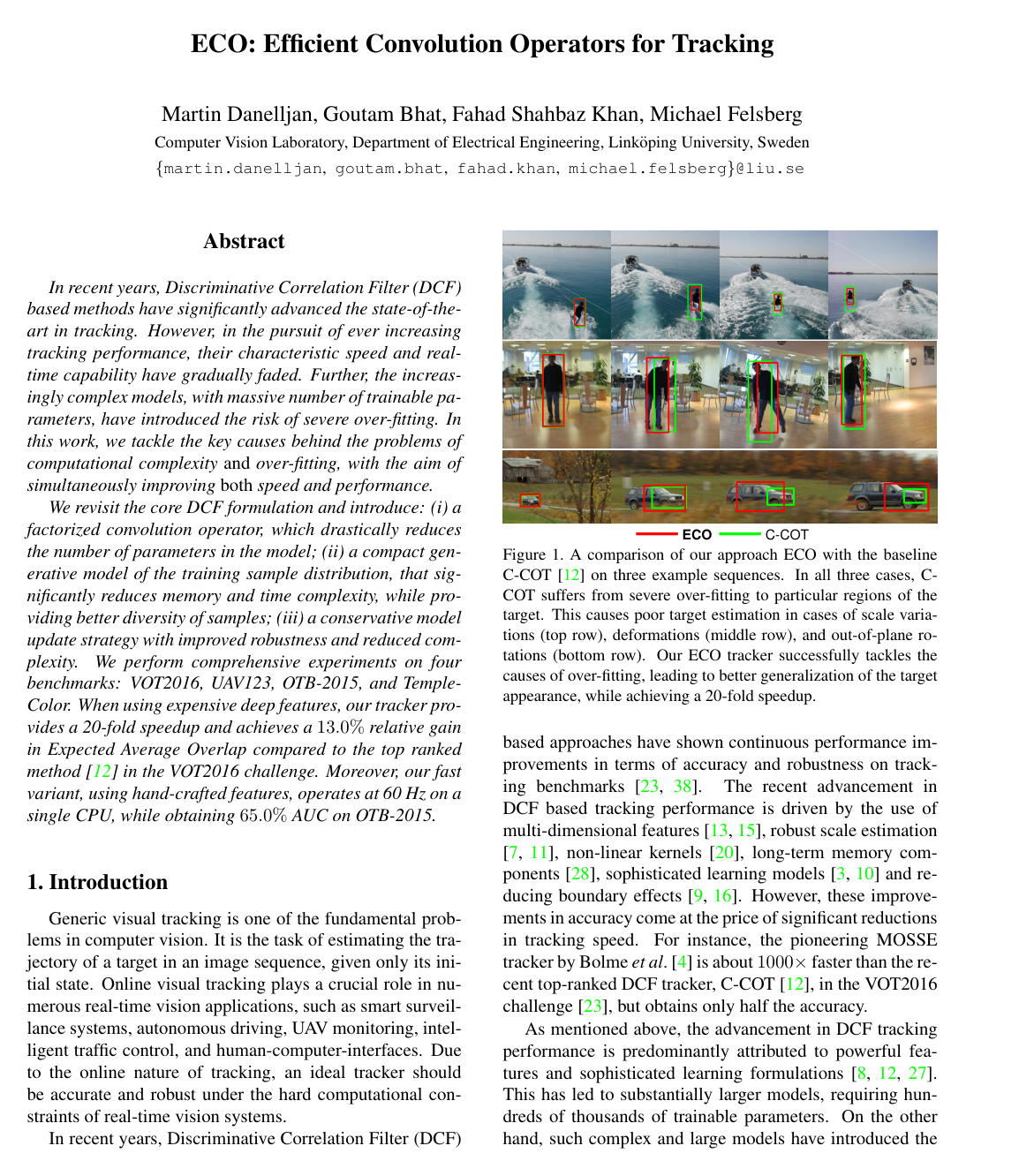
In recent years, Discriminative Correlation Filter (DCF) based methods have significantly advanced the state-of-the-art in tracking. However, in the pursuit of ever increasing tracking performance, their characteristic speed and real-time capability have gradually faded. Further, the increasingly complex models, with massive number of trainable parameters, have introduced the risk of severe over-fitting. In this work, we tackle the key causes behind the problems of computational complexity and over-fitting, with the aim of simultaneously improving both speed and performance.

We revisit the core DCF formulation and introduce: (i) a factorized convolution operator, which drastically reduces the number of parameters in the model; (ii) a compact generative model of the training sample distribution, that significantly reduces memory and time complexity, while providing better diversity of samples; (iii) a conservative model update strategy with improved robustness and reduced complexity. We perform comprehensive experiments on four benchmarks: VOT2016, UAV123, OTB-2015, and TempleColor. When using expensive deep features, our tracker provides a 20-fold speedup and achieves a 13.0% relative gain in Expected Average Overlap compared to the top ranked method in the VOT2016 challenge. Moreover, our fast variant, using hand-crafted features, operates at 60 Hz on a single CPU, while obtaining 65.0% AUC on OTB-2015.

Topics

correlation coefficient cpu generative model tracking performance training sample

Keywords

efficient convolution operators visual tracking discriminative correlation filter continuous convolution deep features basis filters conjugate gradient iterations

1 Introduction
1.1 Motivation
1.2 Contributions
2 Baseline Approach: C-COT
3 Our Approach
3.1 Factorized Convolution Operator
3.2 Generative Sample Space Model
3.3 Model Update Strategy
4 Experiments
4.1 Implementation Details
4.2 Baseline Comparison
4.3 State-of-the-art Comparison
5 Conclusions
References

Knowls

Knowl 1 — Factorized Continuous Convolution Operator
model/method
In Continuous Convolution Operator Tracking (C-COT), multi-channel feature maps $x$ with channel dimensions $d \in \{1, \dots, D\}$ and layer resolutions $N_d$ are interpolated into the continuous spatial domain $t \in [0, T)$ via periodic interpolation kernels $b_d$ with period $T > 0$ :

$J_d\{x^d\}(t) = \sum_{n=0}^{N_d-1} x^d[n] b_d\left(t - \frac{T}{N_d}n\right)$

where $J\{x\}(t) = (J_1\{x^1\}(t), \dots, J_D\{x^D\}(t))^T \in \mathbb{R}^D$ .

Instead of learning an independent continuous filter $f^d$ for each channel $d \in \{1, \dots, D\}$ , the factorized convolution formulation represents the target model using a smaller set of $C < D$ basis filters $f = (f^1, \dots, f^C)$ and a learned projection matrix $P = (p_{d,c}) \in \mathbb{R}^{D \times C}$ . The continuous target detection score is computed as:

$S_{Pf}\{x\}(t) = (Pf * J\{x\})(t) = \sum_{c=1}^C \sum_{d=1}^D p_{d,c} (f^c * J_d\{x^d\})(t) = (f * P^T J\{x\})(t)$

where $(f * g)(t) = \frac{1}{T} \int_0^T f(t - \tau) g(\tau) d\tau$ denotes continuous circular convolution on $[0, T)$ . This decomposes filter evaluation into a spatial linear dimensionality reduction $P^T J\{x\}(t) \in \mathbb{R}^C$ followed by convolution with the $C$ basis filters $f$ .
Knowl 2 — Gauss-Newton Optimization of the Factorized Operator in the Fourier Domain
model/method
Given an interpolated sample feature map $z = J\{x\}$ , let $\hat{z}^d[k] = X^d[k] \hat{b}_d[k]$ denote the Fourier coefficients of channel $d$ , where $X^d$ is the Discrete Fourier Transform of $x^d$ and $\hat{b}_d[k] = \frac{1}{T} \int_0^T b_d(t) e^{-i \frac{2\pi}{T} kt} dt$ . The joint training objective for the basis filters $f$ and projection matrix $P$ in the Fourier domain is:

$E(f, P) = \|\hat{z}^T P \hat{f} - \hat{y}\|_{\ell_2}^2 + \sum_{c=1}^C \|\hat{w} * \hat{f}^c\|_{\ell_2}^2 + \lambda \|P\|_F^2$

where $\hat{f}$ and $\hat{y}$ are vectorizations of the Fourier series coefficients of $f$ and the desired Gaussian target scores $y$ , $\hat{w}$ represents Fourier coefficients of a spatial regularization window, and $\lambda > 0$ is a Frobenius norm regularization parameter on $P$ .

Because the term $\hat{z}^T P \hat{f}$ is bilinear, the loss is minimized in the first frame using the Gauss-Newton method. At iteration $i$ , the residual is linearized around current estimates $(\hat{f}_i, P_i)$ via a first-order Taylor expansion:

$\hat{z}^T(P_i + \Delta P)(\hat{f}_i + \Delta \hat{f}) \approx \hat{z}^T P_i \hat{f}_{i,\Delta} + (\hat{f}_i \otimes \hat{z})^T \text{vec}(\Delta P)$

where $\hat{f}_{i,\Delta} = \hat{f}_i + \Delta \hat{f}$ , $\otimes$ is the Kronecker product, and $\Delta p = \text{vec}(\Delta P)$ . Setting the gradient of the resulting quadratic subproblem to zero yields the normal equations:

$\begin{bmatrix} A_P^H A_P + W^H W & A_P^H B_f \\ B_f^H A_P & B_f^H B_f + \lambda I \end{bmatrix} \begin{bmatrix} \hat{f} \\ \Delta p \end{bmatrix} = \begin{bmatrix} A_P^H \hat{y} \\ B_f^H \hat{y} - \lambda p \end{bmatrix}$

where $p = \text{vec}(P_i)$ , $W$ is the convolution matrix with kernel $\hat{w}$ , and $A_P, B_f$ are block matrices containing the linearizations of $\hat{z}^T P_i$ and $(\hat{f}_i \otimes \hat{z})^T$ . Each subproblem is solved using Conjugate Gradient. The projection matrix $P$ is learned in the initial frame and kept fixed thereafter, allowing subsequent frames to update only $f$ on the lower-dimensional projected features $P^T J\{x\}$ .
Knowl 3 — Generative Gaussian Mixture Model for Training Sample Distribution
model/method
To prevent overfitting to recent tracking frames and eliminate sample redundancy in memory, filter learning is framed as minimizing the expected loss over the continuous joint probability distribution $p(x, y)$ of feature maps $x$ and Gaussian label scores $y$ :

$E(f) = \mathbb{E}_{p(x,y)}\left[ \|S_f\{x\} - y\|_{L^2}^2 \right] + \sum_{d=1}^D \|w f^d\|_{L^2}^2$

Because target label scores differ only by a translation aligning the peak to the target center, target centering of the feature map $x$ allows fixing the label function to a common Gaussian $y_0$ , factorizing the joint distribution as $p(x, y) = p(x) \delta_{y_0}(y)$ . The sample feature map distribution $p(x)$ is modeled as a Gaussian Mixture Model (GMM) with $L$ components:

$p(x) = \sum_{l=1}^L \pi_l \mathcal{N}(x; \mu_l; I)$

where $\pi_l \ge 0$ (with $\sum_{l=1}^L \pi_l = 1$ ) is the prior weight of component $l$ , $\mu_l$ is the mean feature map, and the covariance matrix is set to the identity matrix $I$ .

Evaluating the expectation over this generative model converts the expected loss into a weighted sum over the $L$ Gaussian component means:

$E(f) = \sum_{l=1}^L \pi_l \|S_f\{\mu_l\} - y_0\|_{L^2}^2 + \sum_{d=1}^D \|w f^d\|_{L^2}^2$

replacing the $M$ individual historical training samples with $L \ll M$ component centers.
Knowl 4 — Online GMM Sample Maintenance and Component Merging Algorithm
algorithm
The Gaussian Mixture Model representing the training sample distribution is updated online upon receiving each new frame sample $x_j$ , with a component limit $L$ and learning rate $\gamma$ :
Input: New sample feature map $x_j$ , learning rate $\gamma$ , maximum components $L$ , pruning threshold $\tau_{prune}$
Output: Updated GMM components with weights and means $\{(\pi_l, \mu_l)\}_{l=1}^{L'}$ , $L' \le L$
for each existing component $l$ in GMM do
     $\pi_l \leftarrow (1 - \gamma) \pi_l$
end for
Initialize new component $m$ with weight $\pi_m = \gamma$ and mean $\mu_m = x_j$
Add component $m$ to GMM
if number of components in GMM $> L$ then
    for each component $l$ in GMM do
        if $\pi_l < \tau_{prune}$ then
            Discard component $l$ from GMM
        end if
    end for
    if number of components in GMM $> L$ then
        Compute pairwise Fourier distances $\|\mu_k - \mu_l\|$ for all pairs $(k, l)$
        Identify closest pair $(k^*, l^*) = \arg\min_{k \neq l} \|\mu_k - \mu_l\|$
        Merge components $k^*$ and $l^*$ into a single component $n$ :
             $\pi_n = \pi_{k^*} + \pi_{l^*}$
             $\mu_n = \frac{\pi_{k^*} \mu_{k^*} + \pi_{l^*} \mu_{l^*}}{\pi_{k^*} + \pi_{l^*}}$
        Replace $k^*$ and $l^*$ with component $n$ in GMM
    end if
end if
Normalize weights such that $\sum_l \pi_l = 1$
The pairwise distances $\|\mu_k - \mu_l\|$ are computed in the Fourier domain via Parseval's formula.
Knowl 5 — Sparse Frame Interval Model Update Strategy
model/method
Rather than updating the filter parameters in every single frame ( $N_S = 1$ ), the appearance filter optimization is executed sparsely once every $N_S$ frames (with $N_S = 6$ ). The generative sample space model (GMM) continues to be updated on every individual frame, allowing the tracker to aggregate an $N_S$ -frame mini-batch of target information before initiating optimization.

On update frames ( $t \equiv 0 \pmod{N_S}$ ), a fixed budget of $N_{CG} = 5$ Conjugate Gradient iterations is performed to refine the filter $f$ . This reduces the average number of Conjugate Gradient iterations per frame to $N_{CG} / N_S = 5/6 \approx 0.83$ .

To accelerate convergence in the presence of dynamically shifting objectives, the Conjugate Gradient solver uses the Polak-Ribière formula for computing the momentum direction update parameter $\beta_k$ :

$\beta_k^{PR} = \frac{r_k^T (r_k - r_{k-1})}{r_{k-1}^T r_{k-1}}$

where $r_k$ is the residual vector at CG iteration $k$ , improving optimization speed over the standard Fletcher-Reeves formulation.
Knowl 6 — Computational Complexity Reduction in Continuous DCF Optimization
theoretical result
In the baseline Continuous Convolution Operator Tracker (C-COT), solving the linear system for filter parameters with the Conjugate Gradient (CG) method has a learning complexity of $\mathcal{O}(N_{CG} D M \bar{K})$ per frame, where $N_{CG}$ is the number of CG iterations, $D$ is the number of feature channels, $M$ is the number of stored training samples, and $\bar{K} = \frac{1}{D} \sum_{d=1}^D K_d$ is the average number of non-zero Fourier coefficients per channel with bandwidth $K_d = \lfloor N_d / 2 \rfloor$ .

The ECO framework reduces this complexity across all three leading factors:
1. Factorized convolution projects $D$ feature channels into $C$ basis filters ( $C < D$ ), replacing factor $D$ with $C$ and yielding a complexity reduction of $D / C \approx 6\times$ .
2. The generative GMM replaces the $M$ stored samples with $L$ mixture components ( $L < M$ ), reducing complexity by $M / L = 400 / 50 = 8\times$ .
3. The sparse model update executes $N_{CG}$ iterations once every $N_S$ frames, reducing the average iterations per frame to $N_{CG} / N_S$ , giving an additional reduction of $N_S = 6\times$ .
The resulting average learning complexity per frame is $\mathcal{O}\left(\frac{N_{CG}}{N_S} C L \bar{K}\right)$ , achieving a theoretical learning speedup of approximately $(D/C) \times (M/L) \times N_S \approx 6 \times 8 \times 6 = 288\times$ over the baseline learning step.

Knowl 7 — Component Ablation on VOT2016 Dataset

data/table

Configuration	Baseline C-COT	+ Factorized Conv	+ Sample Space Model	+ Model Update (ECO)
EAO	0.331	0.342	0.352	0.374
Speed (FPS, single CPU)	0.3	1.1	2.6	6.0
Complexity change	—	$D \to C$	$M \to L$	$N_{CG} \to N_{CG} / N_S$
Complexity reduction	—	$6\times$	$8\times$	$6\times$

The table demonstrates the cumulative impact of adding each of the three proposed contributions on the 60-sequence VOT2016 benchmark. Performance is measured using Expected Average Overlap (EAO) and processing speed in Frames Per Second (FPS) on a single 4-core Intel Core i7-6700 CPU at 3.4 GHz (excluding feature extraction time).

Integrating the factorized convolution ( $D \to C$ ) improves EAO from 0.331 to 0.342 while increasing speed by $3.7\times$ (0.3 to 1.1 FPS). Adding the generative GMM sample model ( $M=400 \to L=50$ ) raises EAO to 0.352 and speed to 2.6 FPS. Finally, adding the sparse model update ( $N_S=6$ ) increases EAO to 0.374 (a 13.0% relative improvement over baseline C-COT) and raises tracking speed to 6.0 FPS (a 20-fold cumulative speedup on CPU).

Knowl 8 — Feature Channel Configuration and Hyperparameter Settings

experimental setup

ECO combines deep convolutional features from the VGG-m network (Conv-1 and Conv-5 layers) with hand-crafted features (HOG and Color Names). Across all modalities, total input dimensionality $D = 96 + 512 + 31 + 11 = 650$ is factorized into $C = 16 + 64 + 10 + 3 = 93$ basis filters, reducing model filter parameters by 85.7%.

Key tracker hyperparameters include:

Projection matrix regularization weight: $\lambda = 2 \cdot 10^{-7}$ .
Initial frame optimization: 10 Gauss-Newton iterations, each using 20 Conjugate Gradient iterations for the quadratic subproblem. Basis filter Fourier coefficients $\hat{f}_0$ are initialized to 0; projection matrix $P_0$ is initialized using Principal Component Analysis (PCA).
Sample space model: learning rate $\gamma = 0.012$ , maximum number of Gaussian components $L = 50$ (compared to $M = 400$ in C-COT).
Model update interval: $N_S = 6$ frames.
Online Conjugate Gradient iterations: $N_{CG} = 5$ iterations per update step using the Polak-Ribière formula.
Fast variant (ECO-HC): uses only HOG ( $D=31 \to C=10$ ) and Color Names ( $D=11 \to C=3$ ), running at 60 FPS on a single CPU including feature extraction.

Knowl 9 — Tracking Performance on the VOT2016 Benchmark

data/table

Tracker	SRBT	EBT	DDC	Staple	MLDF	SSAT	TCNN	C-COT	ECO-HC	ECO
EAO	0.290	0.291	0.293	0.295	0.311	0.321	0.325	0.331	0.322	0.374
Failure rate	1.25	0.90	1.23	1.35	0.83	1.04	0.96	0.85	1.08	0.72
Accuracy	0.50	0.44	0.53	0.54	0.48	0.57	0.54	0.52	0.53	0.54
Speed (EFO)	3.69	3.01	0.20	11.14	1.48	0.48	1.05	0.51	15.13	4.53

The table reports performance on the VOT2016 dataset (60 challenging sequences) evaluated according to Expected Average Overlap (EAO), failure rate (robustness), tracking accuracy (average overlap on successfully tracked frames), and tracking speed in Equivalent Filter Operations (EFO).

ECO achieves the top EAO score of 0.374 (a 13.0% relative improvement over C-COT at 0.331) and the lowest failure rate of 0.72. ECO operates at 4.53 EFO, representing an 8.9-fold speedup over C-COT (0.51 EFO) and a 4.3-fold speedup over TCNN (1.05 EFO). The hand-crafted variant ECO-HC achieves 0.322 EAO at the highest frame rate among top trackers (15.13 EFO).

Knowl 10 — Tracking Evaluation on UAV123, OTB-2015, and TempleColor Datasets
empirical result
ECO and its fast hand-crafted variant (ECO-HC) were evaluated against state-of-the-art visual trackers using the Area Under the Curve (AUC) metric of success plots:
- OTB-2015 (100 video sequences): Deep-feature ECO achieves the highest overall AUC of 70.0%, outperforming C-COT (69.0%), MDNet (68.5%), TCNN (66.1%), and DeepSRDCF (64.3%). ECO-HC obtains 65.0% AUC while operating at 60 FPS on a single CPU, surpassing all compared hand-crafted trackers including SRDCFad (63.4%), SRDCF (60.5%), and Staple (58.4%).
- UAV123 (123 aerial video sequences, >110K frames): ECO achieves 53.7% AUC, outperforming C-COT (51.7%). The real-time ECO-HC variant achieves 51.7% AUC at 60 FPS on CPU, outperforming real-time Staple (45.3% AUC) by 6.4 percentage points.
- TempleColor (128 video sequences): ECO achieves 60.5% AUC, outperforming C-COT (59.7%), ECO-HC (55.8%), DeepSRDCF (54.3%), and SRDCFad (54.1%).

Coverage note — No substantial contributed material was omitted from the extracted knowls.

References

1.L. Bertinetto, J. Valmadre, S. Golodetz, O. Miksik, and P. H. S. Torr. Staple: Complementary learners for real-time tracking. In CVPR, 2016.
2.L. Bertinetto, J. Valmadre, J. F. Henriques, A. Vedaldi, and P. H. Torr. Fully-convolutional siamese networks for object tracking. In ECCV workshop, 2016.
3.A. Bibi, M. Mueller, and B. Ghanem. Target response adaptation for correlation filter tracking. In ECCV, 2016.
4.D. S. Bolme, J. R. Beveridge, B. A. Draper, and Y. M. Lui. Visual object tracking using adaptive correlation filters. In CVPR, 2010.
5.K. Chatfield, K. Simonyan, A. Vedaldi, and A. Zisserman. Return of the devil in the details: Delving deep into convolutional nets. In BMVC, 2014.
6.N. Dalal and B. Triggs. Histograms of oriented gradients for human detection. In CVPR, 2005.
7.M. Danelljan, G. H"ager, F. Shahbaz Khan, and M. Felsberg. Accurate scale estimation for robust visual tracking. In BMVC, 2014.
8.M. Danelljan, G. H"ager, F. Shahbaz Khan, and M. Felsberg. Convolutional features for correlation filter based visual tracking. In ICCV Workshop, 2015.
9.M. Danelljan, G. H"ager, F. Shahbaz Khan, and M. Felsberg. Learning spatially regularized correlation filters for visual tracking. In ICCV, 2015.
10.M. Danelljan, G. H"ager, F. Shahbaz Khan, and M. Felsberg. Adaptive decontamination of the training set: A unified formulation for discriminative visual tracking. In CVPR, 2016.
11.M. Danelljan, G. H"ager, F. Shahbaz Khan, and M. Felsberg. Discriminative scale space tracking. TPAMI, PP(99), 2016.
12.M. Danelljan, A. Robinson, F. Shahbaz Khan, and M. Felsberg. Beyond correlation filters: Learning continuous convolution operators for visual tracking. In ECCV, 2016.
13.M. Danelljan, F. Shahbaz Khan, M. Felsberg, and J. van de Weijer. Adaptive color attributes for real-time visual tracking. In CVPR, 2014.
14.A. Declercq and J. H. Piater. Online learning of gaussian mixture models - a two-level approach. In VISAPP, 2008.
15.H. K. Galoogahi, T. Sim, and S. Lucey. Multi-channel correlation filters. In ICCV, 2013.
16.H. K. Galoogahi, T. Sim, and S. Lucey. Correlation filters with limited boundaries. In CVPR, 2015.
17.J. Gao, H. Ling, W. Hu, and J. Xing. Transfer learning based visual tracking with gaussian process regression. In ECCV, 2014.
18.G. H. Golub and Q. Ye. Inexact preconditioned conjugate gradient method with inner-outer iteration. SIAM J. Scientific Computing, 21(4):1305–1320, 1999.
19.S. Hare, A. Saffari, and P. Torr. Struck: Structured output tracking with kernels. In ICCV, 2011.
20.J. F. Henriques, R. Caseiro, P. Martins, and J. Batista. High-speed tracking with kernelized correlation filters. TPAMI, 37(3):583–596, 2015.
21.J. Hyeong Hong and A. Fitzgibbon. Secrets of matrix factorization: Approximations, numerics, manifold optimization and random restarts. In ICCV, 2015.
22.Z. Kalal, J. Matas, and K. Mikolajczyk. P-n learning: Bootstrapping binary classifiers by structural constraints. In CVPR, 2010.
23.M. Kristan, A. Leonardis, J. Matas, R. Felsberg, Pflugfelder, M., L. \v{C}ehovin, G. Voj\v{\i}r, T.and H"ager, and et al. The visual object tracking vot2016 challenge results. In ECCV workshop, 2016.
24.M. Kristan, J. Matas, A. Leonardis, M. Felsberg, L. \v{C}ehovin, G. Fern'andez, T. Voj\v{\i}r, G. Nebehay, R. Pflugfelder, and G. H"ager. The visual object tracking vot2015 challenge results. In ICCV workshop, 2015.
25.Y. Li and J. Zhu. A scale adaptive kernel correlation filter tracker with feature integration. In ECCV Workshop, 2014.
26.P. Liang, E. Blasch, and H. Ling. Encoding color information for visual tracking: Algorithms and benchmark. TIP, 24(12):5630–5644, 2015.
27.C. Ma, J.-B. Huang, X. Yang, and M.-H. Yang. Hierarchical convolutional features for visual tracking. In ICCV, 2015.
28.C. Ma, X. Yang, C. Zhang, and M.-H. Yang. Long-term correlation tracking. In CVPR, 2015.
29.M. Mueller, N. Smith, and B. Ghanem. A benchmark and simulator for uav tracking. In ECCV, 2016.
30.H. Nam, M. Baek, and B. Han. Modeling and propagating cnns in a tree structure for visual tracking. CoRR, abs/1608.07242, 2016.
31.H. Nam and B. Han. Learning multi-domain convolutional neural networks for visual tracking. In CVPR, 2016.
32.J. Nocedal and S. J. Wright. Numerical Optimization. Springer, 2nd edition, 2006.
33.H. Possegger, T. Mauthner, and H. Bischof. In defense of color-based model-free tracking. In CVPR, 2015.
34.J. R. Shewchuk. An introduction to the conjugate gradient method without the agonizing pain. Technical report, Pittsburgh, PA, USA, 1994.
35.J. van de Weijer, C. Schmid, J. J. Verbeek, and D. Larlus. Learning color names for real-world applications. TIP, 18(7):1512–1524, 2009.
36.A. Vedaldi and K. Lenc. Matconvnet – convolutional neural networks for matlab. CoRR, abs/1412.4564, 2014.
37.Y. Wu, J. Lim, and M.-H. Yang. Online object tracking: A benchmark. In CVPR, 2013.
38.Y. Wu, J. Lim, and M.-H. Yang. Object tracking benchmark. TPAMI, 37(9):1834–1848, 2015.
39.J. Zhang, S. Ma, and S. Sclaroff. MEEM: robust tracking via multiple experts using entropy minimization. In ECCV, 2014.
40.G. Zhu, F. Porikli, and H. Li. Beyond local search: Tracking objects everywhere with instance-specific proposals. In CVPR, 2016.

Citation

MLA

Danelljan, M., et al. “ECO: Efficient Convolution Operators for Tracking”. 2017 IEEE Conference on Computer Vision and Pattern Recognition (CVPR), 2017, pp. 6931–39, https://doi.org/10.1109/CVPR.2017.733.

APA

Danelljan, M., Bhat, G., Khan, F. S., & Felsberg, M. (2017). ECO: Efficient Convolution Operators for Tracking. 2017 IEEE Conference on Computer Vision and Pattern Recognition (CVPR), 6931–6939. https://doi.org/10.1109/CVPR.2017.733

Chicago

Danelljan, M., G. Bhat, F. S. Khan, and M. Felsberg. 2017. “ECO: Efficient Convolution Operators for Tracking”. 2017 IEEE Conference on Computer Vision and Pattern Recognition (CVPR), 6931–39. https://doi.org/10.1109/CVPR.2017.733.

Harvard

Danelljan, M. et al. (2017) “ECO: Efficient Convolution Operators for Tracking”, 2017 IEEE Conference on Computer Vision and Pattern Recognition (CVPR). IEEE, pp. 6931–6939. Available at: https://doi.org/10.1109/CVPR.2017.733.

Vancouver

1. Danelljan M, Bhat G, Khan FS, Felsberg M (2017) ECO: Efficient Convolution Operators for Tracking. In: 2017 IEEE Conference on Computer Vision and Pattern Recognition (CVPR). IEEE, pp 6931–6939

BibTeX

@inproceedings{Danelljan_2017, title={ECO: Efficient Convolution Operators for Tracking}, url={http://dx.doi.org/10.1109/CVPR.2017.733}, DOI={10.1109/cvpr.2017.733}, booktitle={2017 IEEE Conference on Computer Vision and Pattern Recognition (CVPR)}, publisher={IEEE}, author={Danelljan, Martin and Bhat, Goutam and Khan, Fahad Shahbaz and Felsberg, Michael}, year={2017}, month=July, pages={6931–6939} }

Metadata:Crossref

Source Code

This paper has an official code repository available. Click below to access the source code.

View Repository

Access the Paper

This paper is available from its original source. Click below to access the PDF.

Open PDF

License: IEEE

Feature Type	Conv-1 (VGG-m)	Conv-5 (VGG-m)	HOG	Color Names (CN)
Feature dimension $D$	96	512	31	11
Filter dimension $C$	16	64	10	3

ECO: Efficient Convolution Operators for Tracking

Abstract

Topics

Keywords

Table of Contents

Knowls

Knowl 1 — Factorized Continuous Convolution Operator

Knowl 2 — Gauss-Newton Optimization of the Factorized Operator in the Fourier Domain

Knowl 3 — Generative Gaussian Mixture Model for Training Sample Distribution

Knowl 4 — Online GMM Sample Maintenance and Component Merging Algorithm

Knowl 5 — Sparse Frame Interval Model Update Strategy

Knowl 6 — Computational Complexity Reduction in Continuous DCF Optimization