Learning Spatially Regularized Correlation Filters for Visual Tracking

Martin DanelljanGustav HägerFahad Shahbaz KhanMichael Felsberg

article2015ICCV1,976 citations

Proposes a spatial regularization formulation for discriminative correlation filters that overcomes boundary effects in visual tracking, allowing models to learn from wider background contexts and achieving substantial accuracy gains across standard benchmarks.

Listen

Visual tracking systems must accurately locate moving targets across video frames using only an initial starting position. A standard class of algorithms, known as discriminative correlation filters, provides high processing speeds by assuming that image samples repeat periodically. However, this periodic assumption introduces artificial boundary distortions that restrict the search window and degrade tracking quality during fast motion, target deformation, and background clutter.

The article evaluates whether introducing a spatial regularization technique can eliminate these boundary errors while preserving high efficiency. The primary objective is to demonstrate that penalizing filter values outside the central target region allows trackers to learn from much larger background contexts without corrupting the core target model.

To achieve this, the authors designed a framework that applies spatial weights directly during the learning process, suppressing background coefficients. By taking advantage of mathematical properties in the frequency domain, they resolved the resulting equations efficiently using the iterative Gauss-Seidel method. The authors also integrated a sub-pixel interpolation method to estimate target positions and scales accurately. They evaluated the tracking system across four standard visual tracking benchmarks containing hundreds of challenging video sequences.

The findings confirm that the proposed tracker delivers substantial performance improvements. On the primary benchmark datasets, the tracker achieved an absolute gain of roughly 8.0% and 8.2% in mean overlap precision over the best existing methods. It also achieved the top overall ranking on both the extensive ALOV++ and VOT2014 challenge datasets. Across detailed attribute tests, the approach outperformed competing algorithms on 10 out of 11 distinct tracking difficulties, showing marked improvements under fast motion, motion blur, and out-of-plane rotations.

These results indicate that spatial regularization successfully resolves the boundary artifacts long associated with correlation filter trackers. For organizations deploying automated video analysis, surveillance, or robotics, adopting this formulation substantially lowers the risk of tracking loss in dynamic environments without requiring high-cost architectural changes. The approach maintains competitive online processing speeds on standard desktop hardware while delivering state-of-the-art accuracy.

Teams implementing real-time computer vision systems should consider integrating spatially regularized filters to improve target tracking reliability. Where high-throughput deployment is required, future development should explore parallelized hardware optimization to boost processing frame rates beyond desktop prototypes. Overall confidence in these performance gains is high due to consistent evaluation across multiple standardized benchmarks.

Linköping University appearance models classifiers computer vision Spatially Regularized Correlation Filters visual tracking Discriminative Correlation Filters

arXiv: 1608.05571 martin-danelljan/ECO

Paper: High-Speed Tracking with Kernelized Correlation Filters, João F. Henriques et al. (2014). This paper establishes the core mathematical framework of discriminative correlation filters using circulant matrices and the discrete Fourier transform, which the source builds directly upon and modifies to penalize boundary effects.
Paper: Exploiting the Circulant Structure of Tracking-by-Detection with Kernels, João F. Henriques et al. (2012). This foundational work introduces the circulant structure and Fourier-domain ridge regression formulations for tracking-by-detection that define the periodic sample assumptions addressed by the source.
Paper: Object Tracking Benchmark, Yi Wu et al. (2015). This benchmark paper establishes the standardized tracking evaluation protocols and benchmark sequences (OTB) utilized in the source's empirical validation.

Paper: ECO: Efficient Convolution Operators for Tracking, Martin Danelljan et al. (2017). This paper extends discriminative correlation filter tracking by introducing factorized convolution operators and compact generative sample models to address the computational overhead and overfitting in multi-channel filter trackers like SRDCF.
Paper: Fully-Convolutional Siamese Networks for Object Tracking, Luca Bertinetto et al. (2016). This work introduces fully-convolutional Siamese architectures that advance correlation-based tracking beyond online-regularized optimization by performing cross-correlation directly via end-to-end offline deep metric learning.
Paper: Learning Multi-domain Convolutional Neural Networks for Visual Tracking, Hyeonseob Nam et al. (2016). This paper advances deep tracking by learning multi-domain convolutional representations with online updates, complementing correlation filter formulations for visual tracking.
Paper: SiamRPN++: Evolution of Siamese Visual Tracking With Very Deep Networks, Bo Li et al. (2018). This work extends Siamese correlation tracking by incorporating deep residual networks and spatial-aware sampling to resolve translation-invariance issues similar to spatial regularizations in tracking.

Cover for Learning Spatially Regularized Correlation Filters for Visual Tracking

Abstract

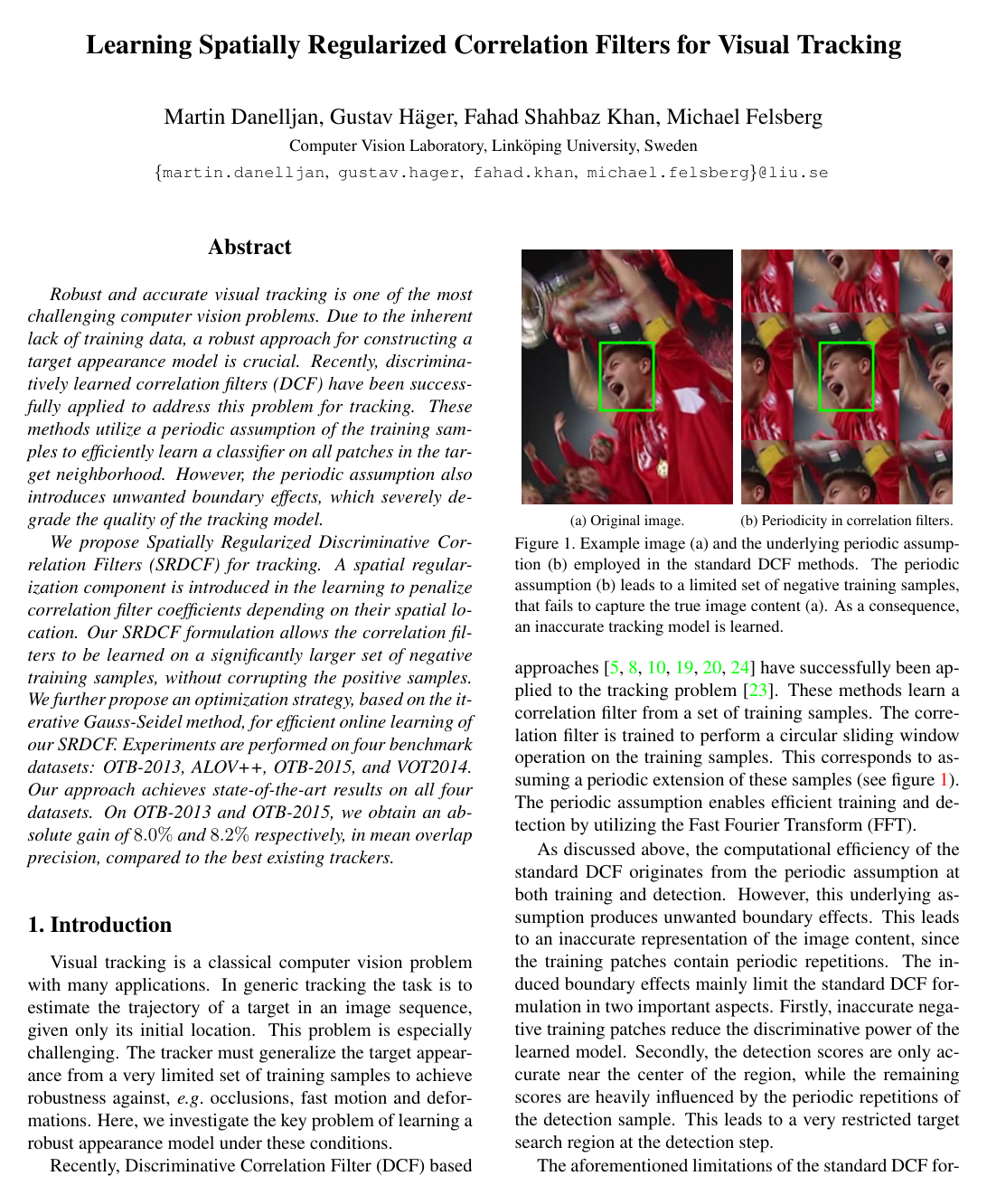
Robust and accurate visual tracking is one of the most challenging computer vision problems. Due to the inherent lack of training data, a robust approach for constructing a target appearance model is crucial. Recently, discriminatively learned correlation filters (DCF) have been successfully applied to address this problem for tracking. These methods utilize a periodic assumption of the training samples to efficiently learn a classifier on all patches in the target neighborhood. However, the periodic assumption also introduces unwanted boundary effects, which severely degrade the quality of the tracking model.

We propose Spatially Regularized Discriminative Correlation Filters (SRDCF) for tracking. A spatial regularization component is introduced in the learning to penalize correlation filter coefficients depending on their spatial location. Our SRDCF formulation allows the correlation filters to be learned on a significantly larger set of negative training samples, without corrupting the positive samples. We further propose an optimization strategy, based on the iterative Gauss-Seidel method, for efficient online learning of our SRDCF. Experiments are performed on four benchmark datasets: OTB-2013, ALOV++, OTB-2015, and VOT2014. Our approach achieves state-of-the-art results on all four datasets. On OTB-2013 and OTB-2015, we obtain an absolute gain of 8.0% and 8.2% respectively, in mean overlap precision, compared to the best existing trackers.

Topics

appearance models classifiers computer vision correlation coefficient filter coefficients online learning optimization regularization training sample object appearance

Keywords

Spatially Regularized Correlation Filters visual tracking Discriminative Correlation Filters spatial regularization component circular correlation scale estimation multi-dimensional features circular convolution

1 Introduction
1.1 Contributions
2 Discriminative Correlation Filters
2.1 Standard DCF Training and Detection
3 Spatially Regularized Correlation Filters
3.1 Spatial Regularization
3.2 Optimization
4 Our Tracking Framework
4.1 Training
4.2 Detection
5 Experiments
5.1 Details and Parameters
5.2 Baseline Comparison
5.3 OTB-2013 Dataset
5.3.1 State-of-the-art Comparison
5.3.2 Robustness to Initialization
5.3.3 Attribute Based Comparison
5.4 OTB-2015 Dataset
5.5 ALOV++ Dataset
5.6 VOT2014 Dataset
6 Conclusions
References

Knowls

Knowl 1 — Spatially Regularized Discriminative Correlation Filter Objective
model/method
The Spatially Regularized Discriminative Correlation Filter (SRDCF) trains a multi-channel circular convolution filter $f = (f^1, \dots, f^d)$ by penalizing the filter coefficients according to their spatial location via a non-uniform weight function $w$ . Given a set of $t$ training samples {x_k}_{k=1}^t where each $x_k$ is a $d$ -dimensional feature map defined over the discrete 2D spatial grid $\Omega = \{0, \dots, M-1\} \times \{0, \dots, N-1\}$ , layer $l \in \{1, \dots, d\}$ is denoted by $x_k^l$ , and the desired scalar label function is $y_k: \Omega \to \mathbb{R}$ .

The circular convolution response of filter $f$ on sample $x$ is defined as:

$S_f(x) = \sum_{l=1}^d x^l * f^l$

where $*$ denotes 2D circular convolution. The SRDCF loss function minimizes the weighted $L^2$ -error on training samples alongside a spatial Tikhonov regularizer:

$\varepsilon(f) = \sum_{k=1}^t \alpha_k \|S_f(x_k) - y_k\|^2 + \sum_{l=1}^d \|w \cdot f^l\|^2$

Here, $\alpha_k \ge 0$ is the sample weight, $\cdot$ denotes point-wise multiplication, and $w: \Omega \to \mathbb{R}$ is a spatial weight function that takes large values in background regions and small values over the target region. When $w(m, n) = \sqrt{\lambda}$ is uniform, the objective reduces to the standard discriminative correlation filter formulation.
Knowl 2 — Spatial Regularization Weight Function Construction and Spectral Sparsification
model/method
To suppress filter coefficients corresponding to background regions while smoothly preserving features inside the target, the spatial regularization function $w(m, n)$ is defined over the 2D grid $\Omega = \{0, \dots, M-1\} \times \{0, \dots, N-1\}$ as a quadratic function centered at the target:

$w(m, n) = \mu + \eta \left(\frac{m}{P}\right)^2 + \eta \left(\frac{n}{Q}\right)^2$

where $P \times Q$ is the spatial size of the target bounding box, $(m, n)$ are spatial coordinates relative to the sample center, $\mu = 0.1$ is the minimum regularization weight assigned at the target center, and $\eta = 3$ controls the penalty impact outside the target region.

To enable computationally efficient Fourier domain optimization, the Discrete Fourier Transform (DFT) $\hat{w} = \mathcal{F}\{w\}$ is sparsified by setting all DFT coefficients with magnitude below a threshold to zero, leaving approximately $K \approx 10$ non-zero Fourier coefficients.
Knowl 3 — Fourier Domain and Real-Valued Formulation of SRDCF Normal Equations
theoretical result
Applying Parseval's theorem to the SRDCF loss function yields the frequency-domain formulation over Hermitian symmetric Discrete Fourier Transform (DFT) filter coefficients $\hat{f}^l = \mathcal{F}\{f^l\}$ :

$\check{\varepsilon}(\hat{f}) = \sum_{k=1}^t \alpha_k \left\| \sum_{l=1}^d D(\hat{x}_k^l) \hat{f}^l - \hat{y}_k \right\|^2 + \sum_{l=1}^d \left\| \frac{C(\hat{w})}{MN} \hat{f}^l \right\|^2$

where $D(v)$ denotes a diagonal matrix with elements of vector $v$ on its diagonal, and $C(\hat{w})$ is the $MN \times MN$ circulant convolution matrix formed by cyclic permutations of the vectorized DFT spectrum $\hat{w}$ .

To enforce Hermitian symmetry and optimize purely over real variables, the grid $\Omega$ is partitioned into $\Omega_0, \Omega_+, \Omega_-$ under the point-reflection $\rho(m,n) = (-m \bmod M, -n \bmod N)$ , and a unitary matrix $B \in \mathbb{C}^{MN \times MN}$ is constructed such that the transformed vector $\tilde{f}^l = B \hat{f}^l \in \mathbb{R}^{MN}$ is real-valued:

$\tilde{f}^l(m, n) = \begin{cases} \hat{f}^l(m, n), & (m, n) \in \Omega_0 \\[6pt] \frac{\hat{f}^l(m, n) + \hat{f}^l(\rho(m, n))}{\sqrt{2}}, & (m, n) \in \Omega_+ \\[6pt] \frac{\hat{f}^l(m, n) - \hat{f}^l(\rho(m, n))}{i\sqrt{2}}, & (m, n) \in \Omega_- \end{cases}$

Defining the real-valued transformed matrices $D_k^l = B D(\hat{x}_k^l) B^H$ , $C = \frac{1}{MN} B C(\hat{w}) B^H$ , the concatenated block matrix $D_k = (D_k^1 \, \dots \, D_k^d)$ , and the $dMN \times dMN$ block diagonal matrix $W = \operatorname{diag}(C, \dots, C)$ , the concatenated real filter $\tilde{f} = ((\tilde{f}^1)^T, \dots, (\tilde{f}^d)^T)^T$ minimizes the real loss $\tilde{\varepsilon}(\tilde{f}) = \sum_{k=1}^t \alpha_k \|D_k \tilde{f} - \tilde{y}_k\|^2 + \|W \tilde{f}\|^2$ .

The resulting normal equations are:

$A_t \tilde{f} = \tilde{b}_t, \quad \text{where } A_t = \sum_{k=1}^t \alpha_k D_k^T D_k + W^T W, \quad \tilde{b}_t = \sum_{k=1}^t \alpha_k D_k^T \tilde{y}_k$

The matrix $A_t$ is sparse, with the fraction of non-zero elements strictly bounded above by $\frac{2d + K^2}{d M N}$ , where $K$ is the number of non-zero Fourier coefficients in $\hat{w}$ .
Knowl 4 — Online Model Update and Gauss-Seidel Optimization Algorithm
algorithm
The online learning of SRDCF updates the normal equations recursively across frames with learning rate $\gamma = 0.025$ and solves for the filter $\tilde{f}_t$ using the iterative Gauss-Seidel method.
Input: Training feature map $x_t$ , label $\tilde{y}_t$ , learning rate $\gamma = 0.025$ , number of iterations $N_{GS} = 4$ , precomputed matrix $W^T W$ , previous state $A_{t-1}, \tilde{b}_{t-1}, \tilde{f}_{t-1}^{(N_{GS})}$
Output: Updated filter coefficients $\tilde{f}_t$ , updated system $A_t, \tilde{b}_t$
Compute Fourier transform $\hat{x}_t$ and construct $D_t = (D_t^1 \dots D_t^d)$
if $t = 1$ then
     $A_1 = D_1^T D_1 + W^T W$
     $\tilde{b}_1 = D_1^T \tilde{y}_1$
    for $l = 1$ to $d$ do
        Solve linear system $(\sum_{p=1}^d (D_1^p)^T D_1^p + d C^T C) \tilde{f}_1^{l,(0)} = (D_1^l)^T \tilde{y}_1$ using direct sparse solver
    end for
     $\tilde{f}_1^{(0)} = ((\tilde{f}_1^{1,(0)})^T, \dots, (\tilde{f}_1^{d,(0)})^T)^T$
else
     $A_t = (1 - \gamma) A_{t-1} + \gamma (D_t^T D_t + W^T W)$
     $\tilde{b}_t = (1 - \gamma) \tilde{b}_{t-1} + \gamma D_t^T \tilde{y}_t$
     $\tilde{f}_t^{(0)} = \tilde{f}_{t-1}^{(N_{GS})}$
end if
Decompose $A_t = L_t + U_t$ into lower triangular $L_t$ and strictly upper triangular $U_t$
for $j = 1$ to $N_{GS}$ do
    Solve $L_t \tilde{f}_t^{(j)} = \tilde{b}_t - U_t \tilde{f}_t^{(j-1)}$ via forward substitution
end for
$\tilde{f}_t = \tilde{f}_t^{(N_{GS})}$
return $\tilde{f}_t, A_t, \tilde{b}_t$
Knowl 5 — Continuous Sub-Grid Detection via Trigonometric Interpolation and Newton's Method
algorithm
When feature extraction uses a spatial stride greater than one pixel, classification scores are initially evaluated on a coarse grid. To estimate the target center with sub-pixel accuracy, the discrete detection scores are interpolated into a continuous trigonometric polynomial using the computed DFT coefficients.

Let $\hat{s}(m, n) = \sum_{l=1}^d \hat{z}^l(m, n) \cdot \hat{f}^l(m, n)$ be the DFT of the correlation response on a test sample $z$ of spatial grid size $M \times N$ . The continuous score function $s(u, v)$ for continuous coordinates $(u, v) \in [0, M) \times [0, N)$ is defined as:

$s(u, v) = \frac{1}{MN} \sum_{m=0}^{M-1} \sum_{n=0}^{N-1} \hat{s}(m, n) e^{i 2\pi \left( \frac{m}{M}u + \frac{n}{N}v \right)}$
Input: DFT response map $\hat{s}$ , grid dimensions $M, N$
Output: Continuous sub-grid peak location $(u^*, v^*)$
Compute coarse discrete grid scores $s(m, n) = \mathcal{F}^{-1}\{\hat{s}\}$ for all $(m, n) \in \Omega$
Initialize $(u^{(0)}, v^{(0)}) = \arg\max_{(m, n) \in \Omega} s(m, n)$
Initialize $k = 0$
while not converged do
    Compute analytical gradient $\nabla s(u^{(k)}, v^{(k)})$ and Hessian $\nabla^2 s(u^{(k)}, v^{(k)})$ by differentiating $s(u, v)$
     $(u^{(k+1)}, v^{(k+1)}) = (u^{(k)}, v^{(k)}) - [\nabla^2 s(u^{(k)}, v^{(k)})]^{-1} \nabla s(u^{(k)}, v^{(k)})$
     $k = k + 1$
end while
$(u^*, v^*) = (u^{(k)}, v^{(k)})$
return $(u^*, v^*)$
Knowl 6 — Multi-Scale Search and SRDCF Computational Complexity
model/method
Scale estimation is performed by extracting test samples $z_r$ across $S$ different scale factors $a^r$ , where $r \in \{\lfloor \frac{1-S}{2} \rfloor, \dots, \lfloor \frac{S-1}{2} \rfloor\}$ and $a$ is the scale increment factor. Each test sample is constructed by resizing the input image prior to feature extraction.

The search image area is set to $4^2 = 16$ times the target bounding box area, with the grid dimensions scaled to ensure a maximum sample size of $M = 50$ cells (using $4 \times 4$ pixel HOG feature cells multiplied by a 2D Hann window). Sub-grid peak detection is performed independently across each of the $S$ scales, and the scale and position achieving the maximum interpolated score update the target state.

Excluding feature extraction, the total computational complexity per frame is:

$\mathcal{O}\left(d S M N \log(MN) + S M N N_{Ne} + (d + K^2) d M N N_{GS}\right)$

where $N_{Ne}$ is the number of Newton iterations in sub-grid detection, $N_{GS} = 4$ is the number of Gauss-Seidel iterations, and $K \approx 10$ is the number of non-zero Fourier coefficients in the regularizer $\hat{w}$ . The complexity is dominated by the filter optimization term $(d + K^2) d M N N_{GS}$ .

Knowl 7 — Impact of Spatial Regularization and Sample Size Expansion

data/table

Comparison of Mean Overlap Precision (OP in %, percentage of frames where bounding box Intersection-over-Union $\ge 0.5$ ) on the OTB-2013 benchmark (50 videos) demonstrates the effect of spatial regularization when expanding the training sample search area.

In standard DCF formulations, expanding the training region from conventional size to an expanded size ( $4^2$ times the target area) causes mean OP to drop sharply from 71.1% to 50.1% because the circular boundary assumption wraps background features into positive training patches. In contrast, the spatial regularization of SRDCF suppresses background filter weights, allowing the model to incorporate negative background context safely and raising mean OP to 78.1% (an absolute gain of 7.0% over conventional DCF).

Under identical single-channel grayscale settings without scale estimation or sub-grid detection, SRDCF achieves 54.3% mean OP compared to 48.6% for Correlation Filters with Limited Boundaries (CFLB), outperforming it by 5.7%.

Knowl 8 — Tracking Performance on OTB-2013 and OTB-2015 Benchmarks

data/table

State-of-the-art comparison on the OTB-2013 (50 videos) and OTB-2015 (100 videos) tracking benchmarks using mean Overlap Precision (OP in %, IoU $\ge 0.5$ ) across top-performing visual tracking methods:

Dataset	LSHT	ASLA	Struck	ACT	TGPR	KCF	DSST	SAMF	MEEM	SRDCF
OTB-2013	47.0	56.4	58.8	52.6	62.6	62.3	67.0	69.7	70.1	78.1
OTB-2015	40.0	49.0	52.9	49.6	54.0	54.9	60.6	64.7	63.4	72.9

SRDCF obtains a mean OP gain of 8.0% on OTB-2013 over the second-best tracker MEEM (70.1%) and an 8.2% gain on OTB-2015 over SAMF (64.7%). In Area Under the Curve (AUC) of the success plot, SRDCF achieves 63.3% on OTB-2013 (outperforming SAMF at 57.7% by 5.6%) and 60.5% on OTB-2015 (outperforming SAMF at 54.8% by 5.7%). Under initialization perturbation protocols on OTB-2013, SRDCF achieves 59.5% AUC under Spatial Robustness Evaluation (SRE) and 65.2% AUC under Temporal Robustness Evaluation (TRE).

Knowl 9 — Tracking Performance on VOT2014 and ALOV++ Benchmarks

data/table

Performance of the top 3 visual trackers on the VOT2014 benchmark (25 videos, evaluated by mean overlap, failure rate, accuracy rank, robustness rank, and combined final rank):

Tracker	Overlap	Failures	Acc. Rank	Rob. Rank	Final Rank
SRDCF	0.63	15.90	6.43	10.08	8.26
DSST	0.64	16.90	5.99	11.17	8.58
SAMF	0.64	19.23	5.87	14.14	10.00

SRDCF achieves the best overall performance with a final rank of 8.26 and the lowest failure rate (15.90).

On the ALOV++ dataset (314 videos, 89,364 frames), SRDCF achieves the highest average F-score of 0.787 on survival curve evaluation, outperforming SAMF (0.772), DSST (0.759), MEEM (0.708), and KCF (0.704).

Coverage note — None was omitted; all key theoretical formulations, mathematical models, algorithms, and benchmark evaluation results from the paper are represented.

References

1.A. Adam, E. Rivlin, and Shimshoni. Robust fragments-based tracking using the integral histogram. In CVPR, 2006.
2.B. Babenko, M.-H. Yang, and S. Belongie. Visual tracking with online multiple instance learning. In CVPR, 2009.
3.C. Bao, Y. Wu, H. Ling, and H. Ji. Real time robust l1 tracker using accelerated proximal gradient approach. In CVPR, 2012.
4.V. N. Boddeti, T. Kanade, and B. V. K. V. Kumar. Correlation filters for object alignment. In CVPR, 2013.
5.D. S. Bolme, J. R. Beveridge, B. A. Draper, and Y. M. Lui. Visual object tracking using adaptive correlation filters. In CVPR, 2010.
6.C. Cortes and V. Vapnik. Support-vector networks. Machine Learning, 20(3):273–297, 1995.
7.N. Dalal and B. Triggs. Histograms of oriented gradients for human detection. In CVPR, 2005.
8.M. Danelljan, G. Hager, F. S. Khan, and M. Felsberg. Accurate scale estimation for robust visual tracking. In BMVC, 2014.
9.M. Danelljan, G. Hager, F. S. Khan, and M. Felsberg. Coloring channel representations for visual tracking. In SCIA, 2015.
10.M. Danelljan, F. S. Khan, M. Felsberg, and J. van de Weijer. Adaptive color attributes for real-time visual tracking. In CVPR, 2014.
11.T. B. Dinh, N. Vo, and G. Medioni. Context tracker: Exploring supporters and distracters in unconstrained environments. In CVPR, 2011.
12.M. Felsberg. Enhanced distribution field tracking using channel representations. In ICCV Workshop, 2013.
13.H. K. Galoogahi, T. Sim, and S. Lucey. Multi-channel correlation filters. In ICCV, 2013.
14.H. K. Galoogahi, T. Sim, and S. Lucey. Correlation filters with limited boundaries. In CVPR, 2015.
15.J. Gao, H. Ling, W. Hu, and J. Xing. Transfer learning based visual tracking with gaussian process regression. In ECCV, 2014.
16.S. Hare, A. Saffari, and P. Torr. Struck: Structured output tracking with kernels. In ICCV, 2011.
17.S. He, Q. Yang, R. Lau, J. Wang, and M.-H. Yang. Visual tracking via locality sensitive histograms. In CVPR, 2013.
18.J. F. Henriques, J. Carreira, R. Caseiro, and J. Batista. Beyond hard negative mining: Efficient detector learning via block-circulant decomposition. In ICCV, 2013.
19.J. F. Henriques, R. Caseiro, P. Martins, and J. Batista. Exploiting the circulant structure of tracking-by-detection with kernels. In ECCV, 2012.
20.J. F. Henriques, R. Caseiro, P. Martins, and J. Batista. High-speed tracking with kernelized correlation filters. PAMI, 2015.
21.X. Jia, H. Lu, and M.-H. Yang. Visual tracking via adaptive structural local sparse appearance model. In CVPR, 2012.
22.Z. Kalal, J. Matas, and K. Mikolajczyk. P-n learning: Bootstrapping binary classifiers by structural constraints. In CVPR, 2010.
23.M. Kristan, R. Pflugfelder, A. Leonardis, J. Matas, and et al. The visual object tracking vot2014 challenge results. In ECCV Workshop, 2014.
24.Y. Li and J. Zhu. A scale adaptive kernel correlation filter tracker with feature integration. In ECCV Workshop, 2014.
25.OpenCV. The opencv state of the art vision challenge. http://code.opencv.org/projects/opencv/wiki/VisionChallenge. Accessed: 2015-09-17.
26.S. Oron, A. Bar-Hillel, D. Levi, and S. Avidan. Locally orderless tracking. In CVPR, 2012.
27.P. Perez, C. Hue, J. Vermaak, and M. Gangnet. Color-based probabilistic tracking. In ECCV, 2002.
28.D. Ross, J. Lim, R.-S. Lin, and M.-H. Yang. Incremental learning for robust visual tracking. IJCV, 77(1):125–141, 2008.
29.L. Sevilla-Lara and E. G. Learned-Miller. Distribution fields for tracking. In CVPR, 2012.
30.A. Smeulders, D. M. Chu, R. Cucchiara, S. Calderara, A. Dehghan, and M. Shah. Visual tracking: An experimental survey. PAMI, 36(7):1442–1468, 2014.
31.J. van de Weijer, C. Schmid, J. J. Verbeek, and D. Larlus. Learning color names for real-world applications. TIP, 18(7):1512–1524, 2009.
32.D. Wang, H. Lu, and M.-H. Yang. Least soft-threshold squares tracking. In CVPR, 2013.
33.Y. Wu, J. Lim, and M.-H. Yang. Online object tracking: A benchmark. In CVPR, 2013.
34.Y. Wu, J. Lim, and M.-H. Yang. Object tracking benchmark. PAMI, 2015.
35.J. Zhang, S. Ma, and S. Sclaroff. MEEM: robust tracking via multiple experts using entropy minimization. In ECCV, 2014.
36.K. Zhang, L. Zhang, and M. Yang. Real-time compressive tracking. In ECCV, 2012.
37.W. Zhong, H. Lu, and M.-H. Yang. Robust object tracking via sparsity-based collaborative model. In CVPR, 2012.

Citation

MLA

Danelljan, M., et al. “Learning Spatially Regularized Correlation Filters for Visual Tracking”. 2015 IEEE International Conference on Computer Vision (ICCV), 2015, pp. 4310–18, https://doi.org/10.1109/ICCV.2015.490.

APA

Danelljan, M., Hager, G., Khan, F. S., & Felsberg, M. (2015). Learning Spatially Regularized Correlation Filters for Visual Tracking. 2015 IEEE International Conference on Computer Vision (ICCV), 4310–4318. https://doi.org/10.1109/ICCV.2015.490

Chicago

Danelljan, M., G. Hager, F. S. Khan, and M. Felsberg. 2015. “Learning Spatially Regularized Correlation Filters for Visual Tracking”. 2015 IEEE International Conference on Computer Vision (ICCV), 4310–18. https://doi.org/10.1109/ICCV.2015.490.

Harvard

Danelljan, M. et al. (2015) “Learning Spatially Regularized Correlation Filters for Visual Tracking”, 2015 IEEE International Conference on Computer Vision (ICCV). IEEE, pp. 4310–4318. Available at: https://doi.org/10.1109/ICCV.2015.490.

Vancouver

1. Danelljan M, Hager G, Khan FS, Felsberg M (2015) Learning Spatially Regularized Correlation Filters for Visual Tracking. In: 2015 IEEE International Conference on Computer Vision (ICCV). IEEE, pp 4310–4318

BibTeX

@inproceedings{Danelljan_2015, title={Learning Spatially Regularized Correlation Filters for Visual Tracking}, url={http://dx.doi.org/10.1109/ICCV.2015.490}, DOI={10.1109/iccv.2015.490}, booktitle={2015 IEEE International Conference on Computer Vision (ICCV)}, publisher={IEEE}, author={Danelljan, Martin and Hager, Gustav and Khan, Fahad Shahbaz and Felsberg, Michael}, year={2015}, month=Dec, pages={4310–4318} }

Metadata:Crossref

Source Code

This paper has an official code repository available. Click below to access the source code.

View Repository

Access the Paper

This paper is available from its original source. Click below to access the PDF.

Open PDF

License: IEEE

	Conventional sample size		Expanded sample size
Regularization	Standard	Ours	Standard	Ours
Mean OP (%)	71.1	72.2	50.1	78.1

Learning Spatially Regularized Correlation Filters for Visual Tracking

Abstract

Topics

Keywords

Table of Contents

Knowls

Knowl 1 — Spatially Regularized Discriminative Correlation Filter Objective

Knowl 2 — Spatial Regularization Weight Function Construction and Spectral Sparsification

Knowl 3 — Fourier Domain and Real-Valued Formulation of SRDCF Normal Equations

Knowl 4 — Online Model Update and Gauss-Seidel Optimization Algorithm

Knowl 5 — Continuous Sub-Grid Detection via Trigonometric Interpolation and Newton's Method

Knowl 6 — Multi-Scale Search and SRDCF Computational Complexity

Knowl 7 — Impact of Spatial Regularization and Sample Size Expansion

Knowl 8 — Tracking Performance on OTB-2013 and OTB-2015 Benchmarks

Knowl 9 — Tracking Performance on VOT2014 and ALOV++ Benchmarks

References

Citation

BibTeX

Source Code

Access the Paper