VolRecon: Volume Rendering of Signed Ray Distance Functions for Generalizable Multi-View Reconstruction

Yufan RenFangjinhua WangTong ZhangMarc PollefeysSabine Süsstrunk

article2023CVPR85 citations

Proposes a generalizable neural implicit reconstruction framework that combines local multi-view projection features with coarse global volume features using signed ray distance functions to recover high-detail surfaces across unseen scenes without per-scene optimization.

Listen

Three-dimensional surface reconstruction from two-dimensional images is a foundational capability for robotics, autonomous navigation, and augmented reality. Recent advances in neural implicit representations have enabled photorealistic image rendering, but existing methods typically require lengthy, per-scene optimization that cannot generalize to unseen environments. Early generalizable implicit reconstruction frameworks often rely on coarse global feature representations that constrain geometric resolution, leading to over-smoothed surfaces and loss of critical spatial detail, especially when only a few input views are available.

The article introduces VolRecon, a neural implicit reconstruction framework designed to reconstruct detailed 3D surfaces across new, unseen scenes without per-scene retraining. The primary objective is to demonstrate that combining directional ray distance formulations with both local and global image features achieves high-fidelity geometry and robust generalization across different scene scales.

The evaluated approach uses a Signed Ray Distance Function (SRDF)—which calculates the shortest distance to a surface along a specific viewing ray—integrated into a volume rendering pipeline. The architecture uses a view transformer to aggregate local multi-view projection features and a ray transformer to process points along a ray alongside global shape priors from a coarse 3D feature volume. The system was trained on the standard indoor DTU dataset using color and depth supervision, and subsequently evaluated on 15 test DTU scenes as well as the larger-scale ETH3D benchmark to measure zero-shot generalization across varying camera viewpoints.

The experimental findings demonstrate significant performance gains over existing approaches. In sparse three-view reconstructions on DTU, VolRecon improved reconstruction accuracy by approximately 30% over the leading generalizable implicit baseline, SparseNeuS, and outperformed the traditional multi-view stereo pipeline COLMAP by about 10%. In full-view reconstructions, VolRecon reduced Chamfer distance errors by roughly 22% compared to SparseNeuS while achieving geometric accuracy comparable to dedicated deep multi-view stereo networks like MVSNet. Depth estimation evaluations showed superior absolute and relative depth accuracy across all benchmark thresholds, while tests on the ETH3D dataset confirmed that the model generalizes directly to large-scale scenes without fine-tuning.

These results indicate that generalizable neural reconstruction can deliver sharp boundaries and fine geometric features without requiring separate optimization cycles for every new target environment. For operational deployments, this capability substantially reduces the computational overhead and latency associated with scene-specific model training, offering a more scalable path for automated mapping and perception pipelines.

For future development, the authors recommend adopting progressive local bounding volume strategies to overcome memory constraints when scaling to very large scenes. Operational users should note that the current rendering speed of approximately 30 seconds per standard-resolution view remains a bottleneck for real-time applications, meaning near-term deployment is best suited for offline or batch reconstruction workflows until rendering efficiency is improved.

École Polytechnique Fédérale de Lausanne ETH Zurich encoder-decoder global feature neural radiance fields multi-view reconstruction signed ray distance functions volume rendering

arXiv: 2212.08067 IVRL/VolRecon

Paper: NeuS: Learning Neural Implicit Surfaces by Volume Rendering for Multi-view Reconstruction, Peng Wang et al. (2021). NeuS establishes the foundational framework for learning neural implicit surfaces via volume rendering of signed distance functions, which VolRecon directly adapts and generalises.
Paper: Volume Rendering of Neural Implicit Surfaces, Lior Yariv et al. (2021). VolSDF provides key theoretical and practical principles for transforming signed distance functions into volumetric densities for neural rendering, underpinning VolRecon's formulation.
Paper: MVSNet: Depth Inference for Unstructured Multi-view Stereo, Yao Yao et al. (2018). MVSNet introduces the global cost volume and multi-view feature aggregation techniques that VolRecon relies upon to construct its coarse global feature volume.
Paper: NeRF: Representing Scenes as Neural Radiance Fields for View Synthesis, Ben Mildenhall et al. (2020). NeRF introduces the fundamental coordinate-based neural radiance field and differentiable volume rendering formulation that neural implicit reconstruction methods build upon.
Paper: pixelNeRF: Neural Radiance Fields from One or Few Images, Alex Yu et al. (2021). pixelNeRF pioneered generalisable, feed-forward neural radiance fields by conditioning continuous representations on extracted multi-view 2D image features.
Paper: DeepSDF: Learning Continuous Signed Distance Functions for Shape Representation, Jeong Joon Park et al. (2019). DeepSDF introduces continuous neural implicit signed distance functions as a powerful representation for high-fidelity 3D shape reconstruction.
Paper: PIFu: Pixel-Aligned Implicit Function for High-Resolution Clothed Human Digitization, Shunsuke Saito et al. (2019). PIFu demonstrates the mechanism of pixel-aligned feature projection to predict continuous implicit 3D geometry from 2D images.

Paper: 2D Gaussian Splatting for Geometrically Accurate Radiance Fields, Binbin Huang et al. (2024). 2D Gaussian Splatting advances geometrically accurate surface reconstruction and fast rendering, offering an alternative explicit primitive formulation compared to generalizable implicit ray marching.
Paper: DUSt3R: Geometric 3D Vision Made Easy, Shuzhe Wang et al. (2023). DUSt3R extends generalizable multi-view 3D reconstruction by regressing dense geometric 3D pointmaps directly from uncalibrated image pairs using transformers.
Paper: VGGT: Visual Geometry Grounded Transformer, Jianyuan Wang et al. (2025). VGGT scales up transformer-based feed-forward multi-view 3D vision to simultaneously predict camera poses, depth maps, and point clouds across many images.
Paper: Depth Pro: Sharp Monocular Metric Depth in Less Than a Second, Alexey Bochkovskiy et al. (2025). Depth Pro builds on modern transformer architectures to deliver zero-shot, sharp metric depth estimation applicable to downstream novel view synthesis and reconstruction workflows.
Paper: Free3D: Consistent Novel View Synthesis Without 3D Representation, Chuanxia Zheng et al. (2024). Free3D explores an alternative paradigm by synthesizing consistent multi-view perspectives via ray-conditioned 2D diffusion without building explicit or implicit 3D volumes.

Cover for VolRecon: Volume Rendering of Signed Ray Distance Functions for Generalizable Multi-View Reconstruction

Abstract

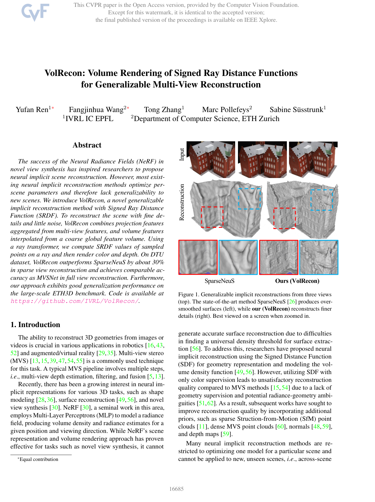
The success of the Neural Radiance Fields (NeRF) in novel view synthesis has inspired researchers to propose neural implicit scene reconstruction. However, most existing neural implicit reconstruction methods optimize per-scene parameters and therefore lack generalizability to new scenes. We introduce VolRecon, a novel generalizable implicit reconstruction method with Signed Ray Distance Function (SRDF). To reconstruct the scene with fine details and little noise, VolRecon combines projection features aggregated from multi-view features, and volume features interpolated from a coarse global feature volume. Using a ray transformer, we compute SRDF values of sampled points on a ray and then render color and depth. On DTU dataset, VolRecon outperforms SparseNeuS by about 30% in sparse view reconstruction and achieves comparable accuracy as MVSNet in full view reconstruction. Furthermore, our approach exhibits good generalization performance on the large-scale ETH3D benchmark. Code is available at https://github.com/IVRL/VolRecon/.

Topics

encoder-decoder global feature neural radiance fields out-of-distribution generalization reconstruction view synthesis viewpoint reconstruction algorithms

Keywords

multi-view reconstruction signed ray distance functions volume rendering neural implicit reconstruction unstructured multi-view stereo generalizable neural rendering novel view synthesis ray transformer ETH3D benchmark

Abstract
1. Introduction
2. Related Work
3. Method
3.1. SRDF Prediction
3.2. Volume Rendering of SRDF
3.3. Loss Function
4. Experiments
4.1. Experimental Settings
4.2. Evaluation Results
4.3. Ablation Study
5. Limitations & Future Work
6. Conclusion
References

Knowls

Knowl 1 — Signed Ray Distance Function Definition and Relation to SDF
definition
Let $\Omega \subset \mathbb{R}^3$ denote a 3D spatial domain and $\mathcal{M} = \partial\Omega$ its boundary surface. The indicator function representing the interior of $\Omega$ for a point $\mathbf{p} \in \mathbb{R}^3$ is defined as:

$\mathbf{1}_{\Omega}(\mathbf{p}) = \begin{cases} 1 & \text{if } \mathbf{p} \in \Omega \\ 0 & \text{if } \mathbf{p} \notin \Omega \end{cases}$

The standard Signed Distance Function (SDF) $d_{\Omega}(\mathbf{p})$ defines the shortest Euclidean distance from $\mathbf{p}$ to the boundary surface $\mathcal{M}$ :

$d_{\Omega}(\mathbf{p}) = (-1)^{\mathbf{1}_{\Omega}(\mathbf{p})} \min_{\mathbf{p}^* \in \mathcal{M}} \|\mathbf{p} - \mathbf{p}^*\|_2$

where $\|\cdot\|_2$ is the $L_2$ -norm and $\mathbf{p}^* \in \mathcal{M}$ are points on the surface.

The Signed Ray Distance Function (SRDF) $\tilde{d}_{\Omega}(\mathbf{p}, \mathbf{v})$ defines the shortest distance from $\mathbf{p}$ to the surface $\mathcal{M}$ restricted along a specific unit ray direction $\mathbf{v} \in \mathbb{R}^3$ with $\|\mathbf{v}\|_2 = 1$ :

$\tilde{d}_{\Omega}(\mathbf{p}, \mathbf{v}) = (-1)^{\mathbf{1}_{\Omega}(\mathbf{p})} \min_{\mathbf{p}^* \in \mathcal{M}, \, \frac{\mathbf{p}^* - \mathbf{p}}{\|\mathbf{p}^* - \mathbf{p}\|_2} = \mathbf{v}} \|\mathbf{p} - \mathbf{p}^*\|_2$

The standard SDF $d_{\Omega}(\mathbf{p})$ is theoretically equal to the minimum absolute SRDF value over all possible ray directions $\mathbf{v}$ :

$d_{\Omega}(\mathbf{p}) = (-1)^{\mathbf{1}_{\Omega}(\mathbf{p})} \min_{\mathbf{v}} (|\tilde{d}_{\Omega}(\mathbf{p}, \mathbf{v})|)$
Knowl 2 — VolRecon Framework Architecture
model/method
VolRecon is a generalizable neural implicit 3D reconstruction model that estimates Signed Ray Distance Function (SRDF) values from multi-view images without requiring per-scene optimization. The framework operates on an input set of $N$ calibrated source images $\mathcal{I} = \{\mathbf{I}_1, \dots, \mathbf{I}_N\}$ with $\mathbf{I}_i \in [0, 1]^{H \times W \times 3}$ and executes the following sequence:
1. Feature Extraction: A 2D Feature Pyramid Network (FPN) extracts multi-scale feature maps $\{\mathbf{F}_i\}_{i=1}^N \in \mathbb{R}^{\frac{H}{4} \times \frac{W}{4} \times C}$ .
2. Global Feature Volume: A coarse 3D bounding grid of $K^3$ voxels aggregates projected multi-view feature statistics (mean and variance), regularized by a 3D U-Net into a volume $\mathbf{F}_v$ to provide global geometry priors $\mathbf{f}_v$ via trilinear interpolation.
3. View Transformer: Sampled 3D points $\mathbf{p}$ along target camera rays are projected onto source views; bilinear-interpolated multi-view features are aggregated using linear self-attention with a learnable token $\mathbf{f}_0$ into local projection features $\mathbf{f}_p$ and updated source features $\{\mathbf{f}'_i\}_{i=1}^N$ .
4. Ray Transformer: Point features along each ray are concatenated as $[\mathbf{f}_v, \mathbf{f}_p, \gamma(t)]$ (where $\gamma(t)$ is positional encoding) and processed across depth samples with linear self-attention along the ray, after which an MLP decodes attended features into scalar SRDF values.
5. Volume Rendering: Radiance is computed by blending source colors using weights derived from $\{\mathbf{f}'_i\}_{i=1}^N$ and view angle differences, and color/depth maps are rendered via NeuS-based logistic density formulation evaluated on SRDF values.
Knowl 3 — Coarse Global Feature Volume Construction
model/method
To provide global shape priors that resolve multi-view ambiguities such as occlusions and textureless regions, VolRecon constructs a global feature volume $\mathbf{F}_v$ :
1. The 3D bounding volume enclosing the scene is partitioned into a uniform voxel grid of resolution $K^3$ (set to $K = 96$ ).
2. The 3D spatial center coordinate of each voxel is projected onto the 2D feature maps $\{\mathbf{F}_i\}_{i=1}^N \in \mathbb{R}^{\frac{H}{4} \times \frac{W}{4} \times C}$ of the $N$ source views.
3. Source features are extracted at projected locations using bilinear interpolation.
4. The element-wise mean and variance across the $N$ extracted feature vectors are computed and concatenated to form the raw voxel feature representation.
5. A 3D U-Net processes and regularizes the voxel grid to produce the final global feature volume $\mathbf{F}_v$ .
6. For any 3D query point $\mathbf{p} \in \mathbb{R}^3$ sampled along a ray, its volume feature $\mathbf{f}_v$ is obtained by querying $\mathbf{F}_v$ through trilinear interpolation.
Knowl 4 — View Transformer for Multi-View Feature and Color Aggregation
model/method
For a given ray emitted from a reference viewpoint, $M$ points $\{\mathbf{p}(t_j) = \mathbf{o} + t_j \mathbf{v}\}_{j=1}^M$ ( $t_j \ge 0$ ) are sampled with origin $\mathbf{o}$ and unit direction $\mathbf{v}$ . Each point $\mathbf{p}$ is projected onto $N$ source views to sample image colors $\{\mathbf{c}_i\}_{i=1}^N$ and 2D FPN features $\{\mathbf{f}_i\}_{i=1}^N$ via bilinear interpolation.

To account for view visibility and occlusions without assuming an ordered view sequence, a View Transformer using linear self-attention aggregates the multi-view features alongside a learnable aggregation token $\mathbf{f}_0$ :

$\mathbf{f}_p, \{\mathbf{f}'_i\}_{i=1}^{N} = \text{ViewTrans}(\mathbf{f}_0, \{\mathbf{f}_i\}_{i=1}^{N})$

where $\mathbf{f}_p$ is the aggregated local projection feature for point $\mathbf{p}$ , and $\{\mathbf{f}'_i\}_{i=1}^N$ are updated multi-view features utilized for dynamic view-dependent color blending. No positional encodings are applied in the View Transformer because the set of input source views is permutation-invariant.
Knowl 5 — Ray Transformer for Non-Local SRDF Feature Aggregation
model/method
Because the Signed Ray Distance Function (SRDF) value depends on the closest surface along a given ray, estimating SRDF at a point requires non-local context across all points sampled along that ray.

For $M$ points sampled along a ray ordered from near to far ( $j = 1, \dots, M$ ), a combined feature vector is formed by concatenating the global volume feature $\mathbf{f}_v$ , the local projection feature $\mathbf{f}_p$ , and a sinusoidal positional encoding $\gamma(t_j)$ of the distance parameter $t_j$ :

$\mathbf{x}_j = \text{cat}(\mathbf{f}_v, \mathbf{f}_p, \gamma(t_j))$

A Ray Transformer applying linear self-attention across the sequential dimension of the $M$ combined point features computes contextually attended features:

$\{\tilde{\mathbf{f}}_j\}_{j=1}^M = \text{RayTrans}\left(\{\mathbf{x}_j\}_{j=1}^M\right)$

Finally, a Multi-Layer Perceptron (MLP) decodes each attended feature $\tilde{\mathbf{f}}_j$ into the predicted scalar SRDF value $\tilde{d}_j$ for the $j$ -th point along the ray.
Knowl 6 — Volume Rendering of SRDF for Color and Depth Estimation
model/method
VolRecon renders color and depth along a camera ray by integrating discrete samples using SRDF-derived densities and dynamic multi-view color blending.

Color Blending: For point $\mathbf{p}$ along viewing direction $\mathbf{v}$ , blending weights $\{\eta_i\}_{i=1}^N$ are computed by concatenating each updated source feature $\mathbf{f}'_i$ with the angular difference $\mathbf{v} - \mathbf{v}_i$ (where $\mathbf{v}_i$ is the ray direction from $\mathbf{p}$ to the $i$ -th source camera), passing the result through an MLP, and applying a Softmax normalization. The blended point color is:

$\hat{\mathbf{c}} = \sum_{i=1}^N \eta_i \cdot \mathbf{c}_i$

Volume Rendering: For $M$ sampled points along the ray with depth parameters $t_1 < t_2 < \dots < t_M$ , the rendered color $\hat{\mathbf{C}}$ and rendered depth $\hat{\mathbf{D}}$ are:

$\hat{\mathbf{C}} = \sum_{j=1}^M T_j \alpha_j \hat{\mathbf{c}}_j, \qquad \hat{\mathbf{D}} = \sum_{j=1}^M T_j \alpha_j t_j$

where discrete accumulative transmittance $T_j$ and opacity $\alpha_j$ are defined as:

$T_j = \prod_{k=1}^{j-1} (1 - \alpha_k), \qquad \alpha_j = 1 - \exp\left(-\int_{t_j}^{t_{j+1}} \rho(t) \, dt\right)$

The density $\rho(t)$ is parameterized using the NeuS logistic density transformation, substituting the conventional SDF with the predicted SRDF $\tilde{d}_{\Omega}(\mathbf{p}(t), \mathbf{v})$ .
Knowl 7 — VolRecon Multi-Task Training Loss Formulation
equation
VolRecon is trained end-to-end using a joint objective function comprising photometric color reconstruction loss and depth supervision loss:

$\mathcal{L} = \mathcal{L}_{\text{color}} + \alpha \mathcal{L}_{\text{depth}}$

where the depth loss weighting hyperparameter is set to $\alpha = 1.0$ .

The color reconstruction loss $\mathcal{L}_{\text{color}}$ is computed as the mean $L_2$ -norm difference between rendered ray colors $\hat{\mathbf{C}}_s$ and ground-truth colors $\mathbf{C}_s$ over $S$ sampled rays:

$\mathcal{L}_{\text{color}} = \frac{1}{S} \sum_{s=1}^S \|\hat{\mathbf{C}}_s - \mathbf{C}_s\|_2$

The depth loss $\mathcal{L}_{\text{depth}}$ is computed as the mean absolute difference ( $L_1$ -norm) between rendered depths $\hat{\mathbf{D}}_s$ and ground-truth depths $\mathbf{D}_s$ over the subset of $S_1$ pixels with valid depth values:

$\mathcal{L}_{\text{depth}} = \frac{1}{S_1} \sum_{s=1}^{S_1} |\hat{\mathbf{D}}_s - \mathbf{D}_s|$

Knowl 8 — Quantitative Evaluation on Sparse-View Reconstruction on the DTU Dataset

data/table

Evaluation of sparse-view 3D surface reconstruction using $N = 3$ input source views on 15 test scans of the DTU benchmark. Reconstructions are evaluated by fusing rendered depth maps using TSDF fusion (voxel size $1.5\text{ mm}$ ) and extracting meshes via Marching Cubes. Results report Chamfer distance in millimeters (lower is better):

Scan	Mean $\downarrow$	24	37	40	55	63	65	69	83	97	105	106	110	114	118	122
COLMAP	1.52	0.90	2.89	1.63	1.08	2.18	1.94	1.61	1.30	2.34	1.28	1.10	1.42	0.76	1.17	1.14
MVSNet	1.22	1.05	2.52	1.71	1.04	1.45	1.52	0.88	1.29	1.38	1.05	0.91	0.66	0.61	1.08	1.16
IDR	3.39	4.01	6.40	3.52	1.91	3.96	2.36	4.85	1.62	6.37	5.97	1.23	4.73	0.91	1.72	1.26
VolSDF	3.41	4.03	4.21	6.12	0.91	8.24	1.73	2.74	1.82	5.14	3.09	2.08	4.81	0.60	3.51	2.18
UNISURF	4.39	5.08	7.18	3.96	5.30	4.61	2.24	3.94	3.14	5.63	3.40	5.09	6.38	2.98	4.05	2.81
NeuS	4.00	4.57	4.49	3.97	4.32	4.63	1.95	4.68	3.83	4.15	2.50	1.52	6.47	1.26	5.57	6.11
PixelNeRF	6.18	5.13	8.07	5.85	4.40	7.11	4.64	5.68	6.76	9.05	6.11	3.95	5.92	6.26	6.89	6.93
IBRNet	2.32	2.29	3.70	2.66	1.83	3.02	2.83	1.77	2.28	2.73	1.96	1.87	2.13	1.58	2.05	2.09
MVSNeRF	2.09	1.96	3.27	2.54	1.93	2.57	2.71	1.82	1.72	2.29	1.75	1.72	1.47	1.29	2.09	2.26
SparseNeuS	1.96	2.17	3.29	2.74	1.67	2.69	2.42	1.58	1.86	1.94	1.35	1.50	1.45	0.98	1.86	1.87
Ours (VolRecon)	1.38	1.20	2.59	1.56	1.08	1.43	1.92	1.11	1.48	1.42	1.05	1.19	1.38	0.74	1.23	1.27

VolRecon achieves an overall mean Chamfer distance of $1.38\text{ mm}$ , outperforming SparseNeuS ( $1.96\text{ mm}$ ) by approximately $30\%$ and surpassing COLMAP ( $1.52\text{ mm}$ ) by roughly $10\%$ .

Knowl 9 — DTU Depth Map Accuracy and Full-View Point Cloud Reconstruction Benchmarks

data/table

VolRecon was evaluated against MVSNet and SparseNeuS on the DTU benchmark across all viewpoints for both depth estimation and full-view point cloud fusion (fusing 49 view depth maps per scan).

Depth Map Evaluation:

Method	$<1\text{mm} \uparrow$	$<2\text{mm} \uparrow$	$<4\text{mm} \uparrow$	Abs. (mm) $\downarrow$	Rel. (%) $\downarrow$
MVSNet	29.95	52.82	72.33	13.62	1.67
SparseNeuS	38.60	56.28	68.63	21.85	2.68
Ours (VolRecon)	44.22	65.62	80.19	7.87	1.00

Threshold percentages ( $<1\text{mm}, <2\text{mm}, <4\text{mm}$ ) and mean absolute relative error (Rel.) are reported in percent; mean absolute error (Abs.) is in millimeters. VolRecon outperforms both MVSNet and SparseNeuS across every depth metric.

Full-View Point Cloud Evaluation:

VolRecon achieves a $0.60\text{ mm}$ Chamfer distance, improving on SparseNeuS ( $0.76\text{ mm}$ , a $22\%$ improvement) and matching the accuracy of MVSNet ( $0.55\text{ mm}$ ).

Knowl 10 — Ablation Analysis of VolRecon Architectural Components and Losses

data/table

Ablation experiments conducted on the DTU dataset analyze the contribution of the Ray Transformer, the coarse global feature volume $\mathbf{F}_v$ , the depth loss $\mathcal{L}_{\text{depth}}$ , and the number of source views $N$ .

Component and Loss Ablations:

	Sparse View	Depth Map Eval.					Full View
Method	Chamfer $\downarrow$	$<1\uparrow$	$<2\uparrow$	$<4\uparrow$	Abs. $\downarrow$	Rel. $\downarrow$	Chamfer $\downarrow$
w/o Ray Trans.	1.79	39.20	60.73	77.38	8.80	1.12	0.66
w/o $\mathbf{F}_v$	1.83	23.29	40.67	59.64	14.90	1.92	0.78
w/o $\mathcal{L}_{\text{depth}}$	2.04	12.84	22.55	34.91	35.00	4.41	1.24
Ours (VolRecon)	1.38	44.22	65.62	80.19	7.87	1.00	0.60

Removing the Ray Transformer restricts SRDF prediction to purely local point information and degrades sparse-view Chamfer distance from $1.38\text{ mm}$ to $1.79\text{ mm}$ . Omitting $\mathbf{F}_v$ removes global shape context, increasing sparse-view Chamfer to $1.83\text{ mm}$ and depth Abs. error to $14.90\text{ mm}$ . Removing depth loss $\mathcal{L}_{\text{depth}}$ severely harms geometry learning, increasing sparse Chamfer distance to $2.04\text{ mm}$ .

Number of Source Views Ablation ( $N$ in Sparse-View DTU):

Reconstruction quality improves monotonically with more input images due to enlarged observed areas and reduced occlusion artifacts.

Knowl 11 — Rendering Speed and Large-Scale Global Volume Scalability Limitations
limitation
VolRecon has two primary documented limitations:
1. Rendering Latency: Due to dense point sampling along rays ( $N_{\text{coarse}} = 64$ and $N_{\text{fine}} = 64$ , totaling $M = 128$ points per ray) and the self-attention mechanisms in the View and Ray Transformers, rendering an $800 \times 600$ image and depth map takes approximately 30 seconds.
2. Scalability on Large-Scale Scenes: The global feature volume $\mathbf{F}_v$ utilizes a fixed cubic resolution of $K^3$ with $K = 96$ . When applied to large-scale scenes, the spatial resolution per voxel decreases, causing representation degradation. Increasing $K$ directly is constrained by cubic memory scaling.

Coverage note — Zero-shot qualitative visualization results on the ETH3D benchmark are omitted as standalone knowls since they are visual examples corroborating the quantitative findings.

References

1.Henrik Aanæs, Rasmus Ramsbøl Jensen, George Vogiatzis, Engin Tola, and Anders Bjorholm Dahl. Large-scale data for multiple-view stereopsis. IJCV, 120:153–168, 2016. 2, 3, 5, 6, 7, 8
2.Jonathan T Barron, Ben Mildenhall, Matthew Tancik, Peter Hedman, Ricardo Martin-Brualla, and Pratul P Srinivasan. Mip-NeRF: A multiscale representation for anti-aliasing neural radiance fields. In ICCV, pages 5855–5864, 2021. 2
3.Eric R Chan, Marco Monteiro, Petr Kellnhofer, Jiajun Wu, and Gordon Wetzstein. pi-GAN: Periodic implicit generative adversarial networks for 3d-aware image synthesis. In CVPR, pages 5799–5809, 2021. 2
4.Anpei Chen, Zexiang Xu, Fuqiang Zhao, Xiaoshuai Zhang, Fanbo Xiang, Jingyi Yu, and Hao Su. MVSNeRF: Fast generalizable radiance field reconstruction from multi-view stereo. In ICCV, pages 14124–14133, 2021. 2, 6, 7, 8
5.Brian Curless and Marc Levoy. A volumetric method for building complex models from range images. In Annual Conference on Computer Graphics and Interactive Techniques, pages 303–312. ACM, 1996. 1, 2, 3, 6, 7
6.Franc¸ois Darmon, Ben´ edicte Bascle, Jean-Cl ´ ement Devaux, ´ Pascal Monasse, and Mathieu Aubry. Improving neural implicit surfaces geometry with patch warping. In CVPR, pages 6260–6269, 2022. 8
7.Alexey Dosovitskiy, Lucas Beyer, Alexander Kolesnikov, Dirk Weissenborn, Xiaohua Zhai, Thomas Unterthiner, Mostafa Dehghani, Matthias Minderer, Georg Heigold, Sylvain Gelly, et al. An image is worth 16x16 words: Transformers for image recognition at scale. CoRR, abs/2010.11929, 2020. 4
8.Arda Duzceker, Silvano Galliani, Christoph Vogel, Pablo Speciale, Mihai Dusmanu, and Marc Pollefeys. DeepVideoMVS: Multi-view stereo on video with recurrent spatio-temporal fusion. In CVPR, pages 15324–15333, 2021. 8
9.William Falcon and The PyTorch Lightning team. PyTorch Lightning, 3 2019. 5
10.Sara Fridovich-Keil, Alex Yu, Matthew Tancik, Qinhong Chen, Benjamin Recht, and Angjoo Kanazawa. Plenoxels: Radiance fields without neural networks. In CVPR, pages 5501–5510, 2022. 2
11.Qiancheng Fu, Qingshan Xu, Yew-Soon Ong, and Wenbing Tao. Geo-Neus: Geometry-consistent neural implicit surfaces learning for multi-view reconstruction. CoRR, abs/2205.15848, 2022. 1, 2, 5, 8
12.Yasutaka Furukawa and Jean Ponce. Accurate, dense, and robust multiview stereopsis. IEEE TPAMI, 32(8):1362–1376, 2009. 2
13.Silvano Galliani, Katrin Lasinger, and Konrad Schindler. Massively parallel multiview stereopsis by surface normal diffusion. In ICCV, pages 873–881, 2015. 1, 2, 6
14.Clement Godard, Oisin Mac Aodha, and Gabriel J Brostow. ´ Unsupervised monocular depth estimation with left-right consistency. In CVPR, pages 270–279, 2017. 8
15.Xiaodong Gu, Zhiwen Fan, Siyu Zhu, Zuozhuo Dai, Feitong Tan, and Ping Tan. Cascade cost volume for high-resolution multi-view stereo and stereo matching. In CVPR, pages 2495–2504, 2020. 1, 3
16.Christian Hane, Torsten Sattler, and Marc Pollefeys. Obstacle ¨ detection for self-driving cars using only monocular cameras and wheel odometry. In International Conference on Intelligent Robots and Systems, pages 5101–5108. IEEE, 2015. 1
17.Sagar Imambi, Kolla Bhanu Prakash, and GR Kanagachidambaresan. Pytorch. In Programming with TensorFlow, pages 87–104. Springer, 2021. 5
18.Shahram Izadi, David Kim, Otmar Hilliges, David Molyneaux, Richard Newcombe, Pushmeet Kohli, Jamie Shotton, Steve Hodges, Dustin Freeman, Andrew Davison, et al. Kinectfusion: real-time 3d reconstruction and interaction using a moving depth camera. In Annual ACM Symposium on User Interface Software and Technology, pages 559–568, 2011. 2
19.Angelos Katharopoulos, Apoorv Vyas, Nikolaos Pappas, and Franc¸ois Fleuret. Transformers are rnns: Fast autoregressive transformers with linear attention. In ICML, volume 119, pages 5156–5165. PMLR, 2020. 4
20.Diederik P. Kingma and Jimmy Ba. Adam: A method for stochastic optimization. In ICLR, 2015. 5
21.Arno Knapitsch, Jaesik Park, Qian-Yi Zhou, and Vladlen Koltun. Tanks and temples: Benchmarking large-scale scene reconstruction. ACM TOG, 36(4):1–13, 2017. 3
22.Ilya Kostrikov, Esther Horbert, and Bastian Leibe. Probabilistic labeling cost for high-accuracy multi-view reconstruction. In CVPR, pages 1534–1541, 2014. 2
23.Kiriakos N Kutulakos and Steven M Seitz. A theory of shape by space carving. IJCV, 38(3):199–218, 2000. 2
24.Maxime Lhuillier and Long Quan. A quasi-dense approach to surface reconstruction from uncalibrated images. IEEE TPAMI, 27(3):418–433, 2005. 2
25.Tsung-Yi Lin, Piotr Dollar, Ross Girshick, Kaiming He, ´ Bharath Hariharan, and Serge Belongie. Feature pyramid networks for object detection. In CVPR, pages 2117–2125, 2017. 3
26.Xiaoxiao Long, Cheng Lin, Peng Wang, Taku Komura, and Wenping Wang. SparseNeuS: Fast generalizable neural surface reconstruction from sparse views. In ECCV, pages 210–227. Springer, 2022. 1, 2, 3, 5, 6, 7
27.William E Lorensen and Harvey E Cline. Marching cubes: A high resolution 3d surface construction algorithm. SIGGRAPH, 21(4):163–169, 1987. 6
28.Lars Mescheder, Michael Oechsle, Michael Niemeyer, Sebastian Nowozin, and Andreas Geiger. Occupancy networks: Learning 3d reconstruction in function space. In CVPR, pages 4460–4470, 2019. 1, 2
29.Sven Middelberg, Torsten Sattler, Ole Untzelmann, and Leif Kobbelt. Scalable 6-dof localization on mobile devices. In ECCV, pages 268–283. Springer, 2014. 1
30.Ben Mildenhall, Pratul P Srinivasan, Matthew Tancik, Jonathan T Barron, Ravi Ramamoorthi, and Ren Ng. NeRF: Representing scenes as neural radiance fields for view synthesis. Communications of the ACM, 65(1):99–106, 2021. 1, 2, 5, 8
31.Thomas Muller, Alex Evans, Christoph Schied, and Alexander ¨ Keller. Instant neural graphics primitives with a multiresolution hash encoding. ACM TOG, 41(4):1–15, 2022. 2
32.Zak Murez, Tarrence van As, James Bartolozzi, Ayan Sinha, Vijay Badrinarayanan, and Andrew Rabinovich. Atlas: End-to-end 3d scene reconstruction from posed images. In ECCV, pages 414–431. Springer, 2020. 2, 3
33.Matthias Nießner, Michael Zollhofer, Shahram Izadi, and ¨ Marc Stamminger. Real-time 3d reconstruction at scale using voxel hashing. ACM TOG, 32(6):1–11, 2013. 2
34.Michael Oechsle, Songyou Peng, and Andreas Geiger. Unisurf: Unifying neural implicit surfaces and radiance fields for multi-view reconstruction. In CVPR, pages 5589–5599, 2021. 6
35.Martin Ralf Oswald, Jan Stuhmer, and Daniel Cremers. Gen- ¨ eralized connectivity constraints for spatio-temporal 3d reconstruction. In ECCV, pages 32–46. Springer, 2014. 1
36.Jeong Joon Park, Peter Florence, Julian Straub, Richard Newcombe, and Steven Lovegrove. DeepSDF: Learning continuous signed distance functions for shape representation. In CVPR, pages 165–174, 2019. 1, 2
37.Songyou Peng, Michael Niemeyer, Lars Mescheder, Marc Pollefeys, and Andreas Geiger. Convolutional occupancy networks. In ECCV, pages 523–540. Springer, 2020. 2
38.Olaf Ronneberger, Philipp Fischer, and Thomas Brox. U-net: Convolutional networks for biomedical image segmentation. In International Conference on Medical Image Computing and Computer-assisted Intervention, pages 234–241. Springer, 2015. 3
39.Johannes L Schonberger, Enliang Zheng, Jan-Michael Frahm, ¨ and Marc Pollefeys. Pixelwise view selection for unstructured multi-view stereo. In ECCV, pages 501–518. Springer, 2016. 1, 2, 3, 4, 6, 8
40.Thomas Schops, Johannes L Schonberger, Silvano Galliani, Torsten Sattler, Konrad Schindler, Marc Pollefeys, and Andreas Geiger. A multi-view stereo benchmark with high-resolution images and multi-camera videos. In CVPR, pages 3260–3269, 2017. 2, 3, 5, 6, 8
41.Steven M Seitz and Charles R Dyer. Photorealistic scene reconstruction by voxel coloring. IJCV, 35(2):151–173, 1999. 2
42.Jiaming Sun, Yiming Xie, Linghao Chen, Xiaowei Zhou, and Hujun Bao. NeuralRecon: Real-time coherent 3d reconstruction from monocular video. In CVPR, pages 15598–15607, 2021. 2, 3, 8
43.Matthew Tancik, Vincent Casser, Xinchen Yan, Sabeek Pradhan, Ben Mildenhall, Pratul P Srinivasan, Jonathan T Barron, and Henrik Kretzschmar. Block-NeRF: Scalable large scene neural view synthesis. In CVPR, pages 8248–8258, 2022. 1
44.Ashish Vaswani, Noam Shazeer, Niki Parmar, Jakob Uszkoreit, Llion Jones, Aidan N Gomez, Łukasz Kaiser, and Illia Polosukhin. Attention is all you need. NeurIPS, 30:5998–6008, 2017. 4
45.Dan Wang, Xinrui Cui, Septimiu Salcudean, and Z Jane Wang. Generalizable neural radiance fields for novel view synthesis with transformer. CoRR, abs/2206.05375, 2022. 4
46.Fangjinhua Wang, Silvano Galliani, Christoph Vogel, and Marc Pollefeys. IterMVS: iterative probability estimation for efficient multi-view stereo. In CVPR, pages 8606–8615, 2022. 3
47.Fangjinhua Wang, Silvano Galliani, Christoph Vogel, Pablo Speciale, and Marc Pollefeys. PatchmatchNet: Learned multi-view patchmatch stereo. In CVPR, pages 14194–14203, 2021. 1, 3, 4
48.Jiepeng Wang, Peng Wang, Xiaoxiao Long, Christian Theobalt, Taku Komura, Lingjie Liu, and Wenping Wang. NeuRIS: Neural reconstruction of indoor scenes using normal priors. In ECCV, pages 139–155. Springer, 2022. 1, 2, 8
49.Peng Wang, Lingjie Liu, Yuan Liu, Christian Theobalt, Taku Komura, and Wenping Wang. NeuS: Learning neural implicit surfaces by volume rendering for multi-view reconstruction. NeurIPS, 34:27171–27183, 2021. 1, 2, 3, 4, 5, 6, 7
50.Qianqian Wang, Zhicheng Wang, Kyle Genova, Pratul P Srinivasan, Howard Zhou, Jonathan T Barron, Ricardo Martin-Brualla, Noah Snavely, and Thomas Funkhouser. IBRNet: Learning multi-view image-based rendering. In CVPR, pages 4690–4699, 2021. 2, 4, 6, 7, 8
51.Yi Wei, Shaohui Liu, Yongming Rao, Wang Zhao, Jiwen Lu, and Jie Zhou. NerfingMVS: Guided optimization of neural radiance fields for indoor multi-view stereo. In ICCV, pages 5610–5619, 2021. 1, 7
52.Stephan Weiss, Davide Scaramuzza, and Roland Siegwart. Monocular-slam–based navigation for autonomous micro helicopters in gps-denied environments. Journal of Field Robotics, 28(6):854–874, 2011. 1
53.Qingshan Xu and Wenbing Tao. Multi-scale geometric consistency guided multi-view stereo. In CVPR, pages 5483–5492, 2019. 2
54.Yao Yao, Zixin Luo, Shiwei Li, Tian Fang, and Long Quan. MVSNet: Depth inference for unstructured multi-view stereo. In ECCV, pages 767–783. Springer, 2018. 1, 2, 3, 4, 5, 6, 7, 8
55.Yao Yao, Zixin Luo, Shiwei Li, Tianwei Shen, Tian Fang, and Long Quan. Recurrent mvsnet for high-resolution multi-view stereo depth inference. In CVPR, pages 5525–5534, 2019. 1, 3
56.Lior Yariv, Jiatao Gu, Yoni Kasten, and Yaron Lipman. Volume rendering of neural implicit surfaces. NeurIPS, 34:4805–4815, 2021. 1, 2, 3, 4, 5, 6, 7
57.Lior Yariv, Yoni Kasten, Dror Moran, Meirav Galun, Matan Atzmon, Basri Ronen, and Yaron Lipman. Multiview neural surface reconstruction by disentangling geometry and appearance. NeurIPS, 33:2492–2502, 2020. 2, 3, 6
58.Alex Yu, Vickie Ye, Matthew Tancik, and Angjoo Kanazawa. pixelNeRF: Neural radiance fields from one or few images. In CVPR, pages 4578–4587, 2021. 2, 6
59.Zehao Yu, Songyou Peng, Michael Niemeyer, Torsten Sattler, and Andreas Geiger. MonoSDF: Exploring monocular geometric cues for neural implicit surface reconstruction. NeurIPS, 2022. 1, 2, 7, 8
60.Jingyang Zhang, Yao Yao, Shiwei Li, Tian Fang, David McKinnon, Yanghai Tsin, and Long Quan. Critical regularizations for neural surface reconstruction in the wild. In CVPR, pages 6270–6279, 2022. 1, 2
61.Jingyang Zhang, Yao Yao, Shiwei Li, Zixin Luo, and Tian Fang. Visibility-aware multi-view stereo network. CoRR, abs/2008.07928, 2020. 3
62.Kai Zhang, Gernot Riegler, Noah Snavely, and Vladlen Koltun. NeRF++: Analyzing and improving neural radiance fields. CoRR, abs/2010.07492, 2020. 1
63.Pierre Zins, Yuanlu Xu, Edmond Boyer, Stefanie Wuhrer, and Tony Tung. Multi-view reconstruction using signed ray distance functions (srdf). CoRR, abs/2209.00082, 2022. 2, 3

Citation

MLA

Ren, Y., et al. “VolRecon: Volume Rendering of Signed Ray Distance Functions for Generalizable Multi-View Reconstruction”. arXiv, 2022, http://arxiv.org/abs/2212.08067v2.

APA

Ren, Y., Wang, F., Zhang, T., Pollefeys, M., & Süsstrunk, S. (2022). VolRecon: Volume Rendering of Signed Ray Distance Functions for Generalizable Multi-View Reconstruction. arXiv. http://arxiv.org/abs/2212.08067v2

Chicago

Ren, Y., F. Wang, T. Zhang, M. Pollefeys, and S. Süsstrunk. 2022. “VolRecon: Volume Rendering of Signed Ray Distance Functions for Generalizable Multi-View Reconstruction”. arXiv. http://arxiv.org/abs/2212.08067v2.

Harvard

Ren, Y. et al. (2022) “VolRecon: Volume Rendering of Signed Ray Distance Functions for Generalizable Multi-View Reconstruction”, arXiv [Preprint]. Available at: http://arxiv.org/abs/2212.08067v2.

Vancouver

1. Ren Y, Wang F, Zhang T, Pollefeys M, Süsstrunk S (2022) VolRecon: Volume Rendering of Signed Ray Distance Functions for Generalizable Multi-View Reconstruction. arXiv

BibTeX

@article{ren2022volrecon,
  title = {VolRecon: Volume Rendering of Signed Ray Distance Functions for Generalizable Multi-View Reconstruction},
  author = {Ren, Yufan and Wang, Fangjinhua and Zhang, Tong and Pollefeys, Marc and Süsstrunk, Sabine},
  year = {2022},
  journal = {arXiv},
  url = {http://arxiv.org/abs/2212.08067v2},
  eprint = {2212.08067}
}

Metadata:arXiv

Source Code

This paper has an official code repository available. Click below to access the source code.

View Repository

Access the Paper

This paper is available from its original source. Click below to access the PDF.

Open PDF

License: IEEE

Method	Accuracy $\downarrow$	Completeness $\downarrow$	Chamfer Distance $\downarrow$
MVSNet	0.55	0.59	0.57
SparseNeuS	0.75	0.76	0.76
Ours (VolRecon)	0.55	0.66	0.60

Number of Views ( $N$ )	Chamfer Distance (mm) $\downarrow$
2	1.72
3	1.38
4	1.35
5	1.33

VolRecon: Volume Rendering of Signed Ray Distance Functions for Generalizable Multi-View Reconstruction

Abstract

Topics

Keywords

Table of Contents

Knowls

Knowl 1 — Signed Ray Distance Function Definition and Relation to SDF

Knowl 2 — VolRecon Framework Architecture

Knowl 3 — Coarse Global Feature Volume Construction

Knowl 4 — View Transformer for Multi-View Feature and Color Aggregation

Knowl 5 — Ray Transformer for Non-Local SRDF Feature Aggregation

Knowl 6 — Volume Rendering of SRDF for Color and Depth Estimation

Knowl 7 — VolRecon Multi-Task Training Loss Formulation

Knowl 8 — Quantitative Evaluation on Sparse-View Reconstruction on the DTU Dataset

Knowl 9 — DTU Depth Map Accuracy and Full-View Point Cloud Reconstruction Benchmarks

Knowl 10 — Ablation Analysis of VolRecon Architectural Components and Losses

Knowl 11 — Rendering Speed and Large-Scale Global Volume Scalability Limitations

References

Citation

BibTeX

Source Code

Access the Paper