ATOM: Accurate Tracking by Overlap Maximization

Martin DanelljanGoutam BhatFahad Shahbaz KhanMichael Felsberg

article2018CVPR1,349 citations

Introduces a real-time visual tracking framework that decouples online target classification from offline bounding box overlap prediction, overcoming the accuracy limits of traditional multi-scale search across major benchmarks.

Listen

Real-time visual object tracking is a critical capability in modern computer vision, supporting applications such as autonomous navigation, video surveillance, and robotics. While recent research has significantly improved tracking robustness against background clutter, progress in target estimation accuracy has stalled. Most state-of-the-art tracking systems rely on simple, rigid multi-scale searches that struggle to accommodate complex transformations like aspect-ratio changes, object rotations, and shape deformations.

The main objective of the article is to introduce and evaluate a visual tracking framework called ATOM (Accurate Tracking by Overlap Maximization). The framework demonstrates that decoupling the tracking pipeline into two dedicated components—one for offline-trained target bounding box estimation and another for online-trained target classification—significantly enhances bounding box accuracy while preserving robust real-time performance.

The researchers designed an architecture built on a shared visual backbone network. The target estimation component is trained offline on large-scale video and object detection datasets to predict the overlap score between candidate bounding boxes and the target using target-specific appearance modulation. During tracking, the bounding box is refined by directly maximizing this predicted overlap. Simultaneously, a compact classification head is trained entirely online to locate the target roughly and reject background distractors. To maintain real-time speed, the team employed an efficient second-order optimization method based on Conjugate Gradient and Gauss-Newton approximations, implemented within standard deep learning tools. The framework was evaluated across five diverse benchmark tracking datasets.

The evaluation produced several key findings. First, ATOM established a new state of the art on all five tested benchmarks. On the large-scale TrackingNet benchmark, it achieved a 70.3% success rate, representing a relative improvement of 15% over the previous leading method. On the LaSOT dataset, it improved success by an absolute 10.0% over the prior best tracker. Second, the dedicated target estimation module proved crucial: replacing it with standard multi-scale search reduced tracking accuracy by 8.6 percentage points and cut high-precision bounding box predictions nearly in half. Third, the system maintained high computational efficiency, running at over 30 frames per second on a standard modern graphics processing unit. Finally, the tracker maintained top performance across 12 challenging operational conditions, including severe viewpoint changes, scale variations, and partial occlusions.

These findings imply that treating target state estimation as a complex, high-level visual task rather than a basic scaling problem yields substantial performance gains without sacrificing operational speed. For engineering and product leaders, this demonstrates that high precision and real-time execution are not mutually exclusive in autonomous visual systems. The framework reduces operational failure risks in complex environments where targets frequently deform or rotate, lowering the need for specialized manual calibration.

Organizations developing or deploying visual tracking systems should consider adopting a two-stream architecture that isolates bounding box estimation from target classification. Development teams can implement ATOM’s modular design using standard deep learning libraries to enhance existing tracking pipelines. When deploying the system, practitioners should pre-train the estimation module on large video datasets to maximize generalizability, though the article demonstrates that even moderately sized datasets deliver competitive results.

The primary limitation noted in the article is that the framework’s high bounding box flexibility can slightly reduce its advantage on constrained datasets where targets maintain rigid, fixed aspect ratios. Additionally, performance relies on initializing from a single annotated frame without extensive domain-specific fine-tuning. Overall, the extensive testing across diverse benchmarks provides high confidence in the methodology's robustness and accuracy for generic visual tracking applications.

ETH Zurich Inception Institute of AI Linköping University classifiers estimation method target state ATOM visual tracking overlap prediction

arXiv: 1811.07628 visionml/pytracking

Paper: ECO: Efficient Convolution Operators for Tracking, Martin Danelljan et al. (2017). Introduces key discriminative correlation filtering techniques that ATOM builds upon for online classification and target localization.
Paper: Beyond Correlation Filters: Learning Continuous Convolution Operators for Visual Tracking, Martin Danelljan et al. (2016). Establishes the continuous convolution framework for multi-resolution deep feature tracking that forms the foundation of modern discriminative trackers like ATOM.
Paper: Learning Spatially Regularized Correlation Filters for Visual Tracking, Martin Danelljan et al. (2015). Develops spatially regularized correlation filters to resolve boundary effects in online visual tracking, a precursor to the online classifier utilized in ATOM.
Paper: Learning Multi-domain Convolutional Neural Networks for Visual Tracking, Hyeonseob Nam et al. (2016). Pioneers online domain-specific classifier fine-tuning using deep convolutional networks for robust distractor-aware visual tracking.
Paper: Fully-Convolutional Siamese Networks for Object Tracking, Luca Bertinetto et al. (2016). Presents the foundational offline-trained Siamese architecture for tracking, which ATOM improves upon by explicitly decoupling classification from bounding-box overlap estimation.
Paper: UnitBox: An Advanced Object Detection Network, Jiahui Yu et al. (2016). Introduces direct Intersection over Union (IoU) optimization for bounding box regression, inspiring ATOM's dedicated overlap-maximization target estimation component.
Paper: High-Speed Tracking with Kernelized Correlation Filters, João F. Henriques et al. (2014). Provides the mathematical groundwork for fast discriminative correlation filter tracking using circulant structures in the frequency domain.
Paper: Object Tracking Benchmark, Yi Wu et al. (2015). Establishes standard single-target tracking evaluation protocols and benchmark methodologies utilized to measure tracking accuracy and robustness.

Paper: Learning Discriminative Model Prediction for Tracking, Goutam Bhat et al. (2019). Extends ATOM's architecture (DiMP) by replacing the online classifier heuristic with an end-to-end trainable discriminative model predictor.
Paper: Transformer Tracking, Xin Chen et al. (2021). Advances deep visual tracking by replacing correlation and standard classification components with transformer-based cross-attention and self-attention feature fusion mechanisms.
Paper: LaSOT: A High-Quality Benchmark for Large-Scale Single Object Tracking, Heng Fan et al. (2018). Provides a large-scale, long-term single-object tracking benchmark that evaluates trackers including ATOM-derived architectures under challenging real-world scenarios.
Paper: GOT-10k: A Large High-Diversity Benchmark for Generic Object Tracking in the Wild, Lianghua Huang et al. (2018). Introduces a high-diversity tracking benchmark with strict zero-class overlap between train and test sets to evaluate modern tracking architectures on unseen generic targets.

Cover for ATOM: Accurate Tracking by Overlap Maximization

Abstract

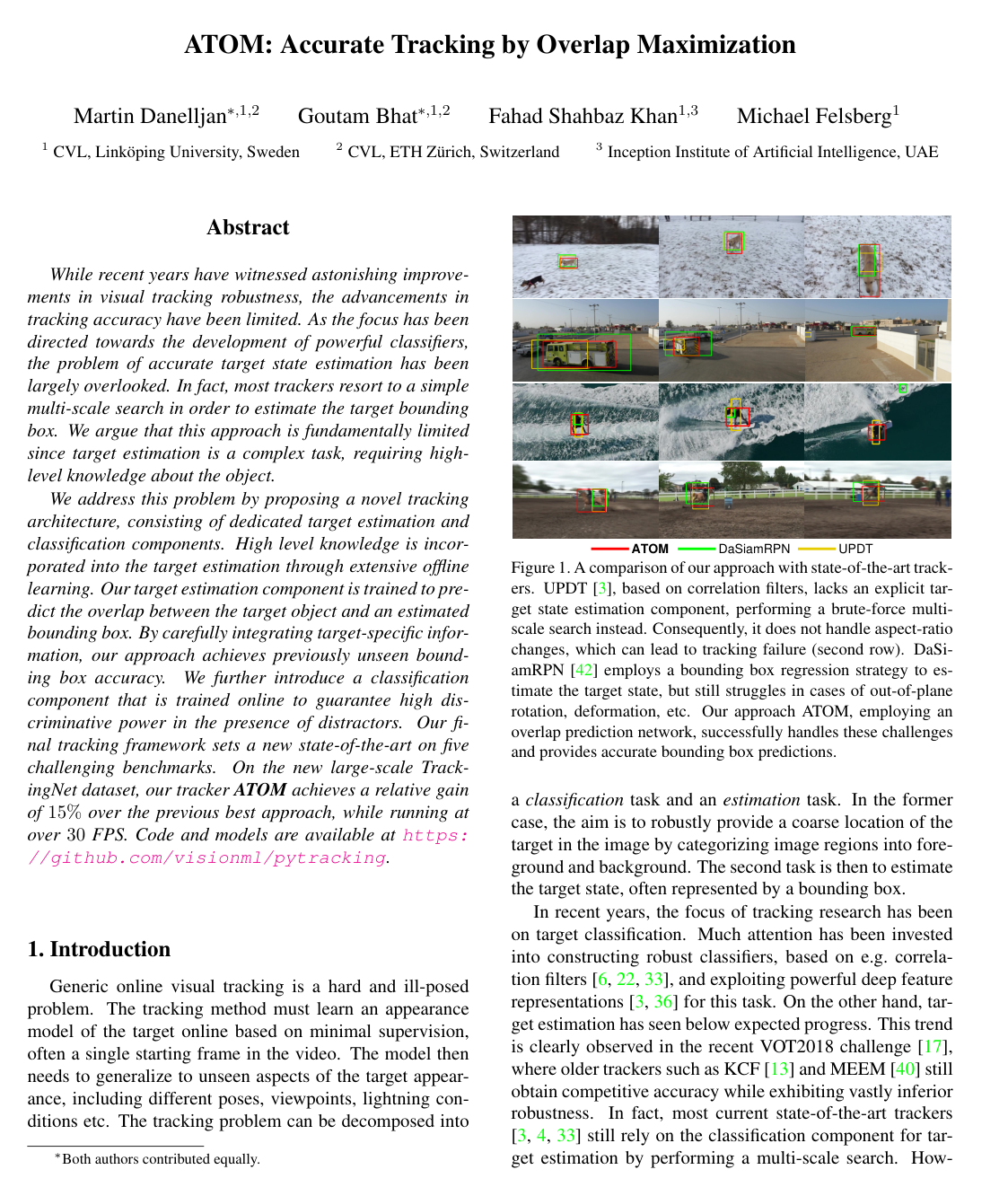
While recent years have witnessed astonishing improvements in visual tracking robustness, the advancements in tracking accuracy have been limited. As the focus has been directed towards the development of powerful classifiers, the problem of accurate target state estimation has been largely overlooked. In fact, most trackers resort to a simple multi-scale search in order to estimate the target bounding box. We argue that this approach is fundamentally limited since target estimation is a complex task, requiring high-level knowledge about the object.

We address this problem by proposing a novel tracking architecture, consisting of dedicated target estimation and classification components. High level knowledge is incorporated into the target estimation through extensive offline learning. Our target estimation component is trained to predict the overlap between the target object and an estimated bounding box. By carefully integrating target-specific information, our approach achieves previously unseen bounding box accuracy. We further introduce a classification component that is trained online to guarantee high discriminative power in the presence of distractors. Our final tracking framework sets a new state-of-the-art on five challenging benchmarks. On the new large-scale TrackingNet dataset, our tracker ATOM achieves a relative gain of 15% over the previous best approach, while running at over 30 FPS. Code and models are available at this https URL.

Topics

classifiers estimation method target state tracking accuracy

Keywords

ATOM visual tracking overlap prediction explicit target state estimation TrackingNet dataset correlation filter tracker bounding box estimation Siamese network

1 Introduction
2 Related Work
3 Proposed Method
3.1 Target Estimation by Overlap Maximization
3.2 Target Classification by Fast Online Learning
3.3 Online Tracking Approach
4 Experiments
4.1 IoU Prediction Architecture Analysis
4.2 Ablation Study
4.3 State-of-the-art Comparison
5 Conclusions
References
S1 Network Architectures for IoU Prediction
S2 Convergence Analysis
S3 Detailed results on LaSOT dataset
S4 Results on OTB-100 dataset
S5 Impact of training data
S6 Additional Results on UAV123

Knowls

Knowl 1 — Two-Component Visual Tracking Framework (ATOM)
model/method
Generic visual object tracking is decomposed into two distinct, dedicated modules operating on deep features extracted from a shared pretrained ResNet-18 backbone network:
1. Target Estimation Module: A network trained offline on large-scale video and object detection datasets to predict the Intersection over Union (IoU) overlap between the target object and an arbitrary candidate bounding box. Target-specific identity is incorporated by modulating test-frame features with target-specific appearance coefficients derived from a reference frame.
2. Target Classification Module: A two-layer fully convolutional neural network trained online to discriminate the target object from background distractors. It outputs a 2D confidence score map over the search area to provide coarse 2D target localization.
During tracking, the shared ResNet-18 backbone extracts Block 3 and Block 4 features from an image patch centered at the previous target estimate (cropped to 5 times the estimated target size and resized to $288 \times 288$ ). The classification module evaluates these features to find the 2D position with maximum confidence. An initial bounding box centered at this location is perturbed to generate multiple candidate boxes, which are refined by maximizing the target estimation module's predicted IoU via gradient ascent. The classification network is updated online using second-order optimization.
Knowl 2 — Modulation-Based Target Estimation Network Architecture
model/method
The target estimation component in ATOM predicts the bounding box overlap (IoU) for generic, unseen targets by conditioning test-frame features on a reference target appearance via channel-wise feature modulation.

The network has two branches fed by features from Block 3 and Block 4 of a ResNet-18 backbone:
- Reference Branch: Takes reference image features $x_0$ and the ground-truth target bounding box $B_0$ . Block 3 and Block 4 features are each passed through a convolutional layer, followed by Precise ROI Pooling (PrPool) layers with spatial resolutions of $3 \times 3$ and $1 \times 1$ , respectively. The pooled features are flattened, concatenated, and passed through a fully connected (FC) layer to produce a target-specific modulation vector $c(x_0, B_0) \in \mathbb{R}^{1 \times 1 \times D_z}$ with positive coefficients.
- Test Branch: Takes test image features $x$ and a candidate bounding box $B = (c_x / w, c_y / h, \log w, \log h)$ , where $(c_x, c_y)$ are image coordinates of the bounding box center and $(w, h)$ are bounding box dimensions. Block 3 and Block 4 features are passed through two convolutional layers and pooled using PrPool layers with spatial resolutions of $5 \times 5$ and $3 \times 3$ , respectively. The outputs are concatenated to produce a feature representation $z(x, B) \in \mathbb{R}^{K \times K \times D_z}$ , where $K$ is the spatial resolution.
- Modulation and Overlap Prediction: The test representation $z(x, B)$ is modulated by the coefficient vector $c(x_0, B_0)$ via channel-wise multiplication:
$z_{\text{mod}}(x, B) = c(x_0, B_0) \cdot z(x, B)$

The modulated feature map $z_{\text{mod}}(x, B)$ is fed into an IoU predictor head $g$ , consisting of three fully connected layers, to output a scalar predicted IoU score:

$\text{IoU}(B) = g(c(x_0, B_0) \cdot z(x, B))$

All convolutional and fully connected layers (except the final output layer) are followed by Batch Normalization and ReLU activations.
Knowl 3 — Target State Refinement via Overlap Maximization
model/method
In the ATOM tracker, target bounding box estimation is performed at test time by continuous optimization of the predicted Intersection over Union (IoU) overlap with respect to bounding box parameters.

Given an initial coarse target center $(c_x, c_y)$ predicted by the target classifier and target dimensions $(w, h)$ from the previous frame, a base bounding box proposal is parameterized as:

$B = \left( \frac{c_x}{w}, \frac{c_y}{h}, \log w, \log h \right) \in \mathbb{R}^4$

To avoid suboptimal local maxima during optimization:
1. A set of 10 initial candidate bounding boxes $\{B^{(i)}\}_{i=1}^{10}$ is generated by adding uniform random noise to the position and scale parameters of $B$ .
2. For each candidate box $B^{(i)}$ , the predicted IoU score $\text{IoU}(B^{(i)}) = g(c(x_0, B_0) \cdot z(x, B^{(i)}))$ is maximized with respect to $B^{(i)}$ using 5 gradient ascent iterations with a step length of 1:
$B^{(i)} \leftarrow B^{(i)} + \nabla_{B^{(i)}} \text{IoU}(B^{(i)})$

Differentiability of the IoU score with respect to $B^{(i)}$ is provided by the continuous Precise ROI Pooling (PrPool) layers in the test branch. 3. The final estimated target state is computed as the arithmetic mean of the coordinates of the 3 candidate bounding boxes that achieve the highest predicted IoU scores after optimization.
Knowl 4 — Online Target Classification Model and Regularized L2 Loss Formulation
equation
The target classification component in the ATOM tracker is a 2-layer fully convolutional neural network designed to discriminate the target object from background distractors. The model is defined as:

$f(x; w) = \phi_2(w_2 * \phi_1(w_1 * x))$

where:
- $x$ is the feature map extracted from Block 4 of the ResNet-18 backbone.
- $w_1$ is a $1 \times 1$ convolutional layer that reduces the feature dimensionality to 64 channels.
- $\phi_1$ is the identity activation function.
- $w_2$ is a $4 \times 4$ convolutional kernel with a single output channel.
- $\phi_2$ is the Parametric Exponential Linear Unit (PELU) activation function, parameterized with $\alpha = 0.05$ :
$\phi_2(t) = \begin{cases} t & \text{if } t \ge 0 \\ \alpha \left(e^{t/\alpha} - 1\right) & \text{if } t < 0 \end{cases}$

The parameters $w = \{w_1, w_2\}$ are learned online by minimizing the regularized $L_2$ objective:

$L(w) = \sum_{j=1}^m \gamma_j \|f(x_j; w) - y_j\|^2 + \sum_k \lambda_k \|w_k\|^2$

where $\{x_j\}_{j=1}^m$ are training sample feature maps, $\gamma_j > 0$ controls the impact of training sample $j$ (updated with a learning rate of $0.01$ ), $\lambda_k$ is the regularization parameter for layer weight $w_k$ , and $y_j \in \mathbb{R}^{W \times H}$ is a target confidence map defined as a 2D Gaussian function centered at the target location.
Knowl 5 — Gauss-Newton Conjugate Gradient Optimization for Online Classifier Learning
algorithm
The online classification loss $L(w) = \|r(w)\|^2$ is minimized using a quadratic Gauss-Newton approximation solved with the Conjugate Gradient (CG) method. The residual vector $r(w)$ is formed by concatenating sample residuals $r_j(w) = \sqrt{\gamma_j}(f(x_j; w) - y_j)$ for $j \in \{1, \dots, m\}$ and regularization residuals $r_{m+k}(w) = \sqrt{\lambda_k} w_k$ for $k \in {1, 2}.

The Gauss-Newton quadratic approximation for parameter increment $\Delta w$ at the current estimate $w$ is:

$\tilde{L}_w(\Delta w) = \Delta w^T J_w^T J_w \Delta w + 2 \Delta w^T J_w^T r_w + r_w^T r_w$

where $r_w = r(w)$ and $J_w = \frac{\partial r}{\partial w}$ is the Jacobian. Matrix-vector operations $J_w p$ and $J_w^T q$ are evaluated using deep learning backpropagation ( $ext{BackProp}(s, v) = \frac{\partial s}{\partial v}$ ):
1. $h = \text{BackProp}(r^T u, w) = J_w^T u$ for $u = r(w)$ .
2. $J_w p = \text{BackProp}(h^T p, u)$ .
3. $J_w^T q_1 = \text{BackProp}(r^T q_1, w)$ for $q_1 = J_w p$ .
Input: Model weights $w$ , residual function $r(w)$ , Gauss-Newton iterations $N_{\text{GN}}$ , Conjugate Gradient iterations $N_{\text{CG}}$
for $i = 1, \dots, N_{\text{GN}}$ do
     $r \leftarrow r(w)$
     $u \leftarrow r$
     $h \leftarrow \text{BackProp}(r^T u, w)$ # Treat $u$ as constant
     $g \leftarrow -h$
     $p \leftarrow 0$
     $\rho_1 \leftarrow 1$
     $\Delta w \leftarrow 0$
    for $n = 1, \dots, N_{\text{CG}}$ do
         $\rho_2 \leftarrow \rho_1$
         $\rho_1 \leftarrow g^T g$
         $\beta \leftarrow \rho_1 / \rho_2$
         $p \leftarrow g + \beta p$
         $q_1 \leftarrow \text{BackProp}(h^T p, u)$ # Treat $p$ as constant
         $q_2 \leftarrow \text{BackProp}(r^T q_1, w)$ # Treat $q_1$ as constant
         $\alpha \leftarrow \rho_1 / (q_2^T p)$
         $g \leftarrow g - \alpha q_2$
         $\Delta w \leftarrow \Delta w + \alpha p$
    end for
     $w \leftarrow w + \Delta w$
end for
return $w$
In the first frame, all classification parameters $w = \{w_1, w_2\}$ are trained with $N_{\text{GN}} = 6$ and $N_{\text{CG}} = 10$ on 30 augmented samples. In subsequent tracking frames, only $w_2$ is updated every 10th frame using $N_{\text{GN}} = 1$ and $N_{\text{CG}} = 5$ .
Knowl 6 — ATOM Online Tracking Procedure with Hard Negative Mining
algorithm
The complete online tracking loop of ATOM alternates between target classification, bounding box estimation, distractor handling, and periodic classifier updates:
Input: Video sequence $\{I_t\}_{t=1}^T$ , initial ground truth bounding box $B_0$ , pretrained ResNet-18 backbone, pretrained IoU prediction network
# Initialization (Frame $t = 1$ )
Extract ResNet-18 Block 3 and Block 4 features $x_0$ from $I_1$
Compute target modulation vector $c(x_0, B_0)$ and cache for tracking
Generate 30 training samples from $I_1$ via translation, rotation, blur, and dropout
Train classifier weights $w = \{w_1, w_2\}$ using Gauss-Newton CG optimization with $N_{\text{GN}} = 6, N_{\text{CG}} = 10$
# Tracking Loop (Frames $t = 2, \dots, T$ )
for $t = 2, \dots, T$ do
    Extract Block 3 and Block 4 features $x$ from a $288 \times 288$ patch centered at the previous target position with 5x target area
    Evaluate classifier $f(x; w) = \phi_2(w_2 * \phi_1(w_1 * x))$ over the search patch
    Locate 2D position $(c_x, c_y)$ corresponding to maximum classification confidence
    Initialize base bounding box proposal $B = (c_x/w_{t-1}, c_y/h_{t-1}, \log w_{t-1}, \log h_{t-1})$
    Sample 10 candidate boxes $\{B^{(i)}\}_{i=1}^{10}$ by adding uniform noise to $B$
    for each candidate $B^{(i)}$ do
        Refine $B^{(i)}$ via 5 gradient ascent steps on $\text{IoU}(B^{(i)}) = g(c(x_0, B_0) \cdot z(x, B^{(i)}))$
    end for
    Set final target state $B_t$ as the mean coordinates of the 3 candidate boxes with highest IoU
    Add sample $x$ labeled with Gaussian $y_t$ at $B_t$ to the training set with learning rate 0.01

    # Hard Negative Mining
    if distractor peak is detected in classification score map then
        Double learning rate weight $\gamma_t$ of current sample
        Update $w_2$ immediately with $N_{\text{GN}} = 1, N_{\text{CG}} = 5$
    end if
    if maximum classification score $< 0.25$ then
        Declare target as lost
    end if

    # Periodic Model Update
    if $t \pmod{10} == 0$ then
        Update $w_2$ using Gauss-Newton CG optimization with $N_{\text{GN}} = 1, N_{\text{CG}} = 5$
    end if
end for
Knowl 7 — Offline Training Setup for the IoU Estimation Network
experimental setup
The target estimation IoU-predictor network is trained offline on bounding-box-annotated image pairs sampled from the training splits of the Large-scale Single Object Tracking (LaSOT) dataset, TrackingNet, and synthetic image pairs from Microsoft COCO:
- Image Pair Sampling: Frame pairs are sampled from video sequences with a maximum temporal separation of 50 frames. From the reference image, a square crop centered at the target with an area of approximately $5^2$ times the target bounding box area is extracted and resized to a fixed resolution. A similar search patch is cropped from the test image with random position and scale perturbations.
- Proposal Generation and Augmentation: For each image pair, 16 candidate bounding boxes are generated on the test patch by adding Gaussian noise to ground-truth coordinates, constrained to maintain an Intersection over Union (IoU) of at least 0.1 with the ground truth. Data augmentation includes horizontal flipping and color jittering.
- Loss Function: Target IoU values are linearly normalized to the range $[-1, 1]$ . The network is trained using mean-squared error (MSE) loss between predicted and normalized ground-truth IoU scores.
- Optimization Parameters: The backbone ResNet-18 weights are kept frozen. The head network is initialized using He normal initialization. Training is conducted for 40 epochs with 64 image pairs per batch using the ADAM optimizer, starting with a learning rate of $10^{-3}$ and decaying by a factor of 0.2 every 15 epochs.

Knowl 8 — Empirical Evaluation of IoU Prediction Architectures and Feature Blocks

data/table

On the combined benchmark consisting of UAV123 (123 videos) and the 30 FPS version of Need for Speed (NFS, 100 videos, 223 videos total), different feature integration architectures and ResNet-18 backbone blocks for offline IoU prediction were evaluated. Performance is reported in Overlap Precision at thresholds 0.50 ( $\text{OP}_{0.50}$ ) and 0.75 ( $\text{OP}_{0.75}$ ), and Area Under the Curve (AUC) of the Success plot:

Architecture	Baseline	Modulation	Concatenation	Siamese	Modulation	Modulation
Backbone Layers	Block 34	Block 34	Block 34	Block 34	Block 3	Block 4
$\text{OP}_{0.50}$ (%)	68.3	76.3	67.5	75.1	73.4	73.6
$\text{OP}_{0.75}$ (%)	38.6	48.4	37.9	47.6	44.5	38.9
AUC (%)	56.7	62.3	56.3	61.7	60.3	58.5

The data demonstrates three key findings:

Necessity of Target Conditioning: Omitting the reference branch entirely (Baseline) lowers AUC by 5.6% (from 62.3% to 56.7%), confirming that general target estimation requires reference appearance conditioning.
Modulation vs. Concatenation and Siamese: Feature modulation outperforms naive feature concatenation (56.3% AUC) and a Siamese dot-product formulation (61.7% AUC).
Multi-Scale Feature Representation: Combining Block 3 and Block 4 features (62.3% AUC) outperforms using Block 3 alone (60.3% AUC) or Block 4 alone (58.5% AUC), showing that multi-scale features provide complementary spatial and semantic information for bounding box overlap prediction.

Knowl 9 — Ablation Study of ATOM Tracking Components

data/table

An ablation study on the combined UAV123 and NFS datasets (223 videos) evaluated the impact of individual components in ATOM against baseline alternatives:

Component	ATOM (Full)	Multi-Scale	No Classif.	GD	GD++	No HN
$\text{OP}_{0.50}$ (%)	76.3	66.2	52.3	74.5	74.8	75.9
$\text{OP}_{0.75}$ (%)	48.4	26.0	35.1	47.4	47.3	48.1
AUC (%)	62.3	53.7	43.0	60.9	61.1	61.9

The ablation results show:

Overlap Maximization vs. Multi-Scale Search: Replacing the overlap maximization module with standard 5-scale correlation filter search (Multi-Scale) causes an 8.6% drop in AUC (62.3% to 53.7%) and cuts $\text{OP}_{0.75}$ from 48.4% to 26.0%, demonstrating the limitation of uniform scale search for complex aspect-ratio and pose variations.
Necessity of Online Classification: Removing the online classification module (No Classif.) and relying solely on the IoU predictor over an expanded search region causes a 19.3% absolute drop in AUC (43.0%), showing vulnerability to background distractors.
Optimization Strategy: Replacing the Gauss-Newton CG algorithm with standard gradient descent (GD, matched in number of backpropagations) degrades AUC from 62.3% to 60.9%. Increasing gradient descent iterations by $5\times$ (GD++) only reaches 61.1% AUC while being significantly slower.
Hard Negative Mining: Disabling hard negative mining (No HN) reduces AUC by 0.4% (to 61.9%).

Knowl 10 — Benchmark Performance Comparison of ATOM Across Tracking Datasets
empirical result
ATOM was evaluated on five visual tracking benchmarks, outperforming state-of-the-art discriminative correlation filter (DCF) and Siamese trackers while operating at over 30 FPS on an Nvidia GTX 1080 GPU:
- TrackingNet (511 test videos): ATOM achieves 64.8% Precision, 77.1% Normalized Precision, and 70.3% Success (AUC), outperforming UPDT (55.7% Prec., 70.2% Norm. Prec., 61.1% Success) by a relative 15.0% gain in Success, as well as MDNet (60.6% Success) and DaSiamRPN (56.8% Success).
- LaSOT (280 test videos): ATOM achieves 57.6% Normalized Precision and 51.5% Success (AUC), surpassing DaSiamRPN (49.6% Norm. Prec., 41.5% Success) with an absolute gain of 10.0% in Success, and outperforming MDNet (39.7% Success) and VITAL (39.0% Success).
- VOT2018 (60 videos): ATOM achieves an Expected Average Overlap (EAO) of 0.401, Accuracy of 0.590, and Robustness (failure rate) of 0.204, outperforming LADCF (EAO 0.389), MFT (EAO 0.385), DaSiamRPN (EAO 0.383, Accuracy 0.586), and UPDT (EAO 0.378).
- Need for Speed (NFS 30 FPS, 100 videos): ATOM achieves 59.0% AUC, outperforming UPDT (54.2% AUC), CCOT (49.2% AUC), ECO (47.0% AUC), and DaSiamRPN (39.5% AUC).
- UAV123 (123 videos): ATOM achieves 65.0% AUC, outperforming DaSiamRPN (58.4% AUC), SiamRPN (57.1% AUC), and UPDT (55.0% AUC).

Coverage note — Omitted detailed per-attribute breakdown plots on UAV123 (12 attributes), OTB-100 benchmark curves, and supplementary ablation using only ImageNet-VID training data (ATOM-VID), as their essential takeaways are fully represented in the primary benchmark results, offline training setup, and ablation knowls.

References

1.L. Bertinetto, J. Valmadre, S. Golodetz, O. Miksik, and P. H. S. Torr. Staple: Complementary learners for real-time tracking. In CVPR, 2016.
2.L. Bertinetto, J. Valmadre, J. F. Henriques, A. Vedaldi, and P. H. Torr. Fully-convolutional siamese networks for object tracking. In ECCV workshop, 2016.
3.G. Bhat, J. Johnander, M. Danelljan, F. S. Khan, and M. Felsberg. Unveiling the power of deep tracking. In ECCV, 2018.
4.M. Danelljan, G. Bhat, F. Shahbaz Khan, and M. Felsberg. ECO: efficient convolution operators for tracking. In CVPR, 2017.
5.M. Danelljan, G. Hager, F. S. Khan, and M. Felsberg. Discriminative scale space tracking. TPAMI, 39(8):1561–1575, 2017.
6.M. Danelljan, G. Hager, F. Shahbaz Khan, and M. Felsberg. Learning spatially regularized correlation filters for visual tracking. In ICCV, 2015.
7.M. Danelljan, A. Robinson, F. Khan, and M. Felsberg. Beyond correlation filters: Learning continuous convolution operators for visual tracking. In ECCV, 2016.
8.H. Fan, L. Lin, F. Yang, P. Chu, G. Deng, S. Yu, H. Bai, Y. Xu, C. Liao, and H. Ling. Lasot: A high-quality benchmark for large-scale single object tracking. In CVPR, 2019.
9.H. K. Galoogahi, A. Fagg, C. Huang, D. Ramanan, and S. Lucey. Need for speed: A benchmark for higher frame rate object tracking. In ICCV, 2017.
10.Q. Guo, W. Feng, C. Zhou, R. Huang, L. Wan, and S. Wang. Learning dynamic siamese network for visual object tracking. In ICCV, 2017.
11.A. He, C. Luo, X. Tian, and W. Zeng. Towards a better match in siamese network based visual object tracker. In ECCV workshop, 2018.
12.K. He, X. Zhang, S. Ren, and J. Sun. Delving deep into rectifiers: Surpassing human-level performance on imagenet classification. In ICCV, 2015.
13.J. F. Henriques, R. Caseiro, P. Martins, and J. Batista. Highspeed tracking with kernelized correlation filters. TPAMI, 37(3):583–596, 2015.
14.P. Jaccard. The distribution of the flora in the alpine zone. New Phytologist, 11(2):37–50, 1912.
15.B. Jiang, R. Luo, J. Mao, T. Xiao, and Y. Jiang. Acquisition of localization confidence for accurate object detection. In ECCV, 2018.
16.D. P. Kingma and J. Ba. Adam: A method for stochastic optimization. In ICLR, 2014.
17.M. Kristan, A. Leonardis, J. Matas, M. Felsberg, R. Pfugfelder, L. C. Zajc, T. Vojir, G. Bhat, A. Lukezic, A. Eldesokey, G. Fernandez, and et al. The sixth visual object tracking vot2018 challenge results. In ECCV workshop, 2018.
18.B. Li, J. Yan, W. Wu, Z. Zhu, and X. Hu. High performance visual tracking with siamese region proposal network. In CVPR, 2018.
19.F. Li, C. Tian, W. Zuo, L. Zhang, and M. Yang. Learning spatial-temporal regularized correlation filters for visual tracking. In CVPR, 2018.
20.Y. Li and J. Zhu. A scale adaptive kernel correlation filter tracker with feature integration. In ECCV workshop, 2014.
21.T. Lin, M. Maire, S. J. Belongie, L. D. Bourdev, R. B. Girshick, J. Hays, P. Perona, D. Ramanan, P. Dollar, and C. L. Zitnick. Microsoft COCO: common objects in context. In ECCV, 2014.
22.A. Lukezic, T. Vojır, L. C. Zajc, J. Matas, and M. Kristan. Discriminative correlation filter tracker with channel and spatial reliability. IJCV, 126(7):671–688, 2018.
23.C. Ma, J.-B. Huang, X. Yang, and M.-H. Yang. Hierarchical convolutional features for visual tracking. In ICCV, 2015.
24.M. Mueller, N. Smith, and B. Ghanem. A benchmark and simulator for uav tracking. In ECCV, 2016.
25.M. Muller, A. Bibi, S. Giancola, S. Al-Subaihi, and B. Ghanem. Trackingnet: A large-scale dataset and benchmark for object tracking in the wild. In ECCV, 2018.
26.H. Nam and B. Han. Learning multi-domain convolutional neural networks for visual tracking. In CVPR, 2016.
27.E. Real, J. Shlens, S. Mazzocchi, X. Pan, and V. Vanhoucke. Youtube-boundingboxes: A large high-precision humanannotated data set for object detection in video. CVPR, 2017.
28.J. Redmon and A. Farhadi. Yolo9000: Better, faster, stronger. In CVPR, 2017.
29.S. Ren, K. He, R. B. Girshick, and J. Sun. Faster R-CNN: towards real-time object detection with region proposal networks. In NIPS, 2015.
30.O. Russakovsky, J. Deng, H. Su, J. Krause, S. Satheesh, S. Ma, Z. Huang, A. Karpathy, A. Khosla, M. Bernstein, A. C. Berg, and L. Fei-Fei. ImageNet Large Scale Visual Recognition Challenge. IJCV, pages 1–42, April 2015.
31.J. R. Shewchuk. An introduction to the conjugate gradient method without the agonizing pain. Technical report, Pittsburgh, PA, USA, 1994.
32.Y. Song, C. Ma, X. Wu, L. Gong, L. Bao, W. Zuo, C. Shen, R. W. H. Lau, and M.-H. Yang. VITAL: Visual tracking via adversarial learning. In CVPR, 2018.
33.C. Sun, D. Wang, H. Lu, and M. Yang. Correlation tracking via joint discrimination and reliability learning. In CVPR, 2018.
34.R. Tao, E. Gavves, and A. W. M. Smeulders. Siamese instance search for tracking. In CVPR, 2016.
35.L. Trottier, P. Giguere, and B. Chaib-draa. Parametric exponential linear unit for deep convolutional neural networks. In ICMLA, 2017.
36.J. Valmadre, L. Bertinetto, J. F. Henriques, A. Vedaldi, and P. H. S. Torr. End-to-end representation learning for correlation filter based tracking. In CVPR, 2017.
37.Y. Wu, J. Lim, and M.-H. Yang. Object tracking benchmark. TPAMI, 37(9):1834–1848, 2015.
38.T. Xu, Z. Feng, X. Wu, and J. Kittler. Learning adaptive discriminative correlation filters via temporal consistency preserving spatial feature selection for robust visual tracking. CoRR, abs/1807.11348, 2018.
39.Y. Yao, X. Wu, S. Shan, and W. Zuo. Joint representation and truncated inference learning for correlation filter based tracking. In ECCV, 2018.
40.J. Zhang, S. Ma, and S. Sclaroff. MEEM: robust tracking via multiple experts using entropy minimization. In ECCV, 2014.
41.Y. Zhang, L. Wang, J. Qi, D. K. Wang, M. Feng, and H. Lu. Structured siamese network for real-time visual tracking. In ECCV, 2018.
42.Z. Zhu, Q. Wang, L. Bo, W. Wu, J. Yan, and W. Hu. Distractor-aware siamese networks for visual object tracking. In ECCV, 2018.

Citation

MLA

Danelljan, M., et al. “ATOM: Accurate Tracking by Overlap Maximization”. arXiv, 2018, http://arxiv.org/abs/1811.07628v2.

APA

Danelljan, M., Bhat, G., Khan, F. S., & Felsberg, M. (2018). ATOM: Accurate Tracking by Overlap Maximization. arXiv. http://arxiv.org/abs/1811.07628v2

Chicago

Danelljan, M., G. Bhat, F. S. Khan, and M. Felsberg. 2018. “ATOM: Accurate Tracking by Overlap Maximization”. arXiv. http://arxiv.org/abs/1811.07628v2.

Harvard

Danelljan, M. et al. (2018) “ATOM: Accurate Tracking by Overlap Maximization”, arXiv [Preprint]. Available at: http://arxiv.org/abs/1811.07628v2.

Vancouver

1. Danelljan M, Bhat G, Khan FS, Felsberg M (2018) ATOM: Accurate Tracking by Overlap Maximization. arXiv

BibTeX

@article{danelljan2018atom,
  title = {ATOM: Accurate Tracking by Overlap Maximization},
  author = {Danelljan, Martin and Bhat, Goutam and Khan, Fahad Shahbaz and Felsberg, Michael},
  year = {2018},
  journal = {arXiv},
  url = {http://arxiv.org/abs/1811.07628v2},
  eprint = {1811.07628}
}

Metadata:arXiv

Source Code

This paper has an official code repository available. Click below to access the source code.

View Repository

Access the Paper

This paper is available from its original source. Click below to access the PDF.

Open PDF

License: IEEE

ATOM: Accurate Tracking by Overlap Maximization

Abstract

Topics

Keywords

Table of Contents

Knowls

Knowl 1 — Two-Component Visual Tracking Framework (ATOM)

Knowl 2 — Modulation-Based Target Estimation Network Architecture

Knowl 3 — Target State Refinement via Overlap Maximization

Knowl 4 — Online Target Classification Model and Regularized L2 Loss Formulation

Knowl 5 — Gauss-Newton Conjugate Gradient Optimization for Online Classifier Learning

Knowl 6 — ATOM Online Tracking Procedure with Hard Negative Mining

Knowl 7 — Offline Training Setup for the IoU Estimation Network