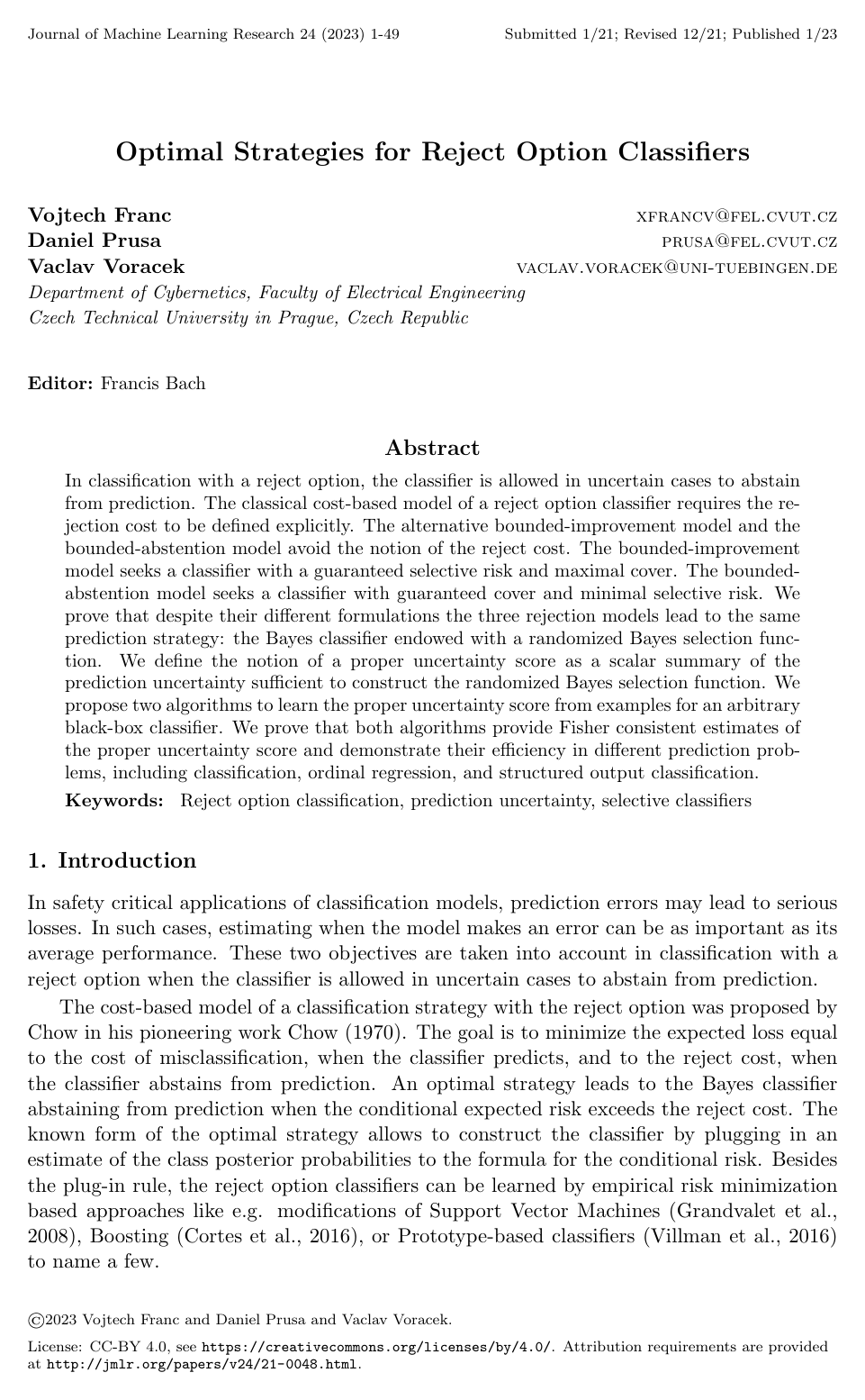
Optimal Strategies for Reject Option Classifiers

Vojtech FrancDaniel PrusaVáclav Vorácek

article2023JMLR62 citations

Unifies cost-based, bounded-improvement, and bounded-abstention selective classification models by proving they share the same optimal strategy, while developing two Fisher consistent algorithms to learn optimal rejection functions for arbitrary black-box classifiers across diverse prediction tasks.

Listen

In safety-critical applications, automated decision models can cause severe operational or financial harm when they make incorrect predictions. To mitigate this risk, systems can use selective classifiers that are permitted to abstain from making a prediction when uncertainty is high. Historically, practitioners relied on three distinct formulations: a cost-based model requiring an explicit financial penalty for abstaining, a bounded-improvement model seeking maximum coverage under a capped error risk, and a bounded-abstention model minimizing risk for a guaranteed coverage level. Defining explicit financial rejection costs is often impractical in real-world scenarios, making the relationship between these formulations and the design of optimal uncertainty scoring mechanisms critical.

The article demonstrates the mathematical equivalence of these three rejection formulations and develops theoretically grounded algorithms to learn uncertainty scores directly from data for any pre-trained, black-box classification model.

To establish these results, the authors mathematically derived the necessary and sufficient optimality conditions for each framework. They introduced two general-purpose learning algorithms to estimate an uncertainty score: one based on loss regression and another based on optimizing a novel smooth surrogate called the Selective Classifier Learning loss. To validate their approach, they performed extensive benchmark experiments using standard machine learning models across 11 standard classification tasks, 11 ordinal regression tasks, and a complex facial landmark detection task.

The analysis produced several key findings. First, all three rejection formulations share an identical underlying optimal decision structure: a base Bayes classifier paired with a randomized threshold rule on the conditional expected risk. Second, minimizing the Selective Classifier Learning loss provably delivers a proper uncertainty score that preserves the optimal ranking of error risks. Third, in classification benchmarks, the Selective Classifier Learning approach achieved the top average rank, significantly outperforming conventional margin-based scores and loss regression. Fourth, in ordinal regression and facial landmark detection, the proposed approach reduced the area under the risk-coverage curve by up to 40 to 50 percent relative to baseline heuristic scores, performing on par with specialized, model-dependent state-of-the-art methods.

These findings provide immediate practical value for managing operational risk and compliance in high-stakes deployments. Decision-makers are no longer forced to assign arbitrary monetary costs to abstentions; they can instead specify straightforward performance targets, such as maximum allowable error or minimum operational coverage. Furthermore, because the proposed scoring algorithms operate on top of existing models without altering their underlying parameters, organizations can enhance legacy predictive systems with reliable abstention capabilities at minimal engineering cost.

For practical implementation, engineering teams deploying black-box models should adopt the Selective Classifier Learning loss algorithm to construct uncertainty scores and tune rejection thresholds using empirical validation sets. When probabilistic models are already in place, simple posterior probability rules remain a viable, low-effort alternative. Future initiatives should focus on developing simultaneous training pipelines that optimize base predictors and uncertainty scores concurrently, as well as scaling non-linear scoring architectures.

Confidence in these theoretical principles and empirical rankings is high across tested benchmark distributions. However, decision-makers should note that the current experimental evaluations rely on linear scoring functions and separate two-stage training datasets. Performance should be verified with domain-specific pilots before broad deployment in production environments.

Czech Technical University in Prague optimal strategies binary classification best response reject option classifiers selective classification optimal selective classifier

arXiv: 2101.12523

Paper: The foundations of cost-sensitive learning, Charles Elkan (2001). It provides the foundational decision-theoretic principles and cost-matrix formulations for cost-sensitive classification that the source paper's cost-based rejection framework directly relies upon.
Paper: Strictly Proper Scoring Rules, Prediction, and Estimation, Tilmann Gneiting et al. (2007). It establishes the mathematical theory of proper scoring rules and uncertainty quantification necessary for defining and estimating proper uncertainty scores in reject-option classifiers.
Paper: Predicting good probabilities with supervised learning, Alexandru Niculescu-Mizil et al. (2005). It analyzes methods for calibrating posterior class probability estimates from black-box classifiers, which underpins the source's approach to learning uncertainty scores.
Paper: MetaCost: a general method for making classifiers cost-sensitive, Pedro M. Domingos (1999). It introduces a framework for converting arbitrary black-box classifiers into cost-sensitive predictors using probability estimations, motivating the source's black-box rejection algorithms.
Paper: Transforming classifier scores into accurate multiclass probability estimates, Bianca Zadrozny et al. (2002). It examines multiclass probability calibration techniques that are critical for deriving proper uncertainty scores across multiclass and structured prediction problems.
Paper: Aleatoric and epistemic uncertainty in machine learning: an introduction to concepts and methods, Eyke Hüllermeier et al. (2019). It offers an extensive conceptual foundation for modeling and quantifying prediction uncertainty in supervised machine learning.

Paper: Two-Stage Learning to Defer with Multiple Experts, Anqi Mao et al. (2023). It generalizes selective prediction and rejection models to two-stage deferral systems involving multiple downstream human or algorithmic experts.

Cover for Optimal Strategies for Reject Option Classifiers

Abstract

In classification with a reject option, the classifier is allowed in uncertain cases to abstain from prediction. The classical cost-based model of a reject option classifier requires the rejection cost to be defined explicitly. The alternative bounded-improvement model and the bounded-abstention model avoid the notion of the reject cost. The bounded-improvement model seeks a classifier with a guaranteed selective risk and maximal cover. The bounded-abstention model seeks a classifier with guaranteed cover and minimal selective risk. We prove that despite their different formulations the three rejection models lead to the same prediction strategy: the Bayes classifier endowed with a randomized Bayes selection function. We define the notion of a proper uncertainty score as a scalar summary of the prediction uncertainty sufficient to construct the randomized Bayes selection function. We propose two algorithms to learn the proper uncertainty score from examples for an arbitrary black-box classifier. We prove that both algorithms provide Fisher consistent estimates of the proper uncertainty score and demonstrate their efficiency in different prediction problems, including classification, ordinal regression, and structured output classification.

Topics

optimal strategies binary classification best response

Keywords

reject option classifiers selective classification optimal selective classifier rejection strategy decision threshold risk minimization Bayes classifier Support Vector Machines ROC analysis

1. Introduction
2. Reject Option Models and Their Optimal Strategies
2.1 Cost-based model
2.2 Bounded-improvement model
2.3 Bounded-abstention model
2.4 Summary
3. Learning uncertainty function
3.1 Area under Risk Coverage curve
3.2 Plug-in conditional risk rule
3.3 Loss regression
3.4 Minimization of SELE loss
4. Related Works
5. Experiments
5.1 Compared methods for uncertainty score learning
5.1.1 Regression score
5.1.2 SELE score
5.1.3 True Class Probability score
5.2 Benchmark problems
5.2.1 Classification
5.2.2 Ordinal regression
5.2.3 Structured Output Classification
5.3 Results
5.3.1 Classification problems
5.3.2 Ordinal regression
5.3.3 Structured Output Classification
6. Conclusions
Acknowledgments
Appendix A. Proofs of theorems from Section 2
A.1 Proof of Theorem 1
A.2 Proof of Theorem 2
A.3 Proof of Theorem 3
A.4 Proof of Theorem 4
A.5 Proof of Theorem 5
A.6 Proof of Theorem 6
Appendix B. Proofs of theorems from Section 3
B.1 Proof of Theorem 7
B.2 Proof of Theorem 8
B.3 Proof of Theorem 9
B.4 Proof of Theorem 11
References

Knowls

Knowl 1 — Unified selective-classification formulation and optimal strategy
model/method
Let $\mathcal X$ be the input space, let $\mathcal Y$ be a finite label set, and let $(X,Y)$ have joint density or mass function $p(x,y)$ . For a loss $\ell:\mathcal Y\times\mathcal Y\to\mathbb R_+$ , a selective classifier consists of a classifier $h:\mathcal X\to\mathcal Y$ and a selection function $c:\mathcal X\to[0,1]$ ; it predicts $h(x)$ with probability $c(x)$ and rejects otherwise. Define the coverage and selective risk by
$\phi(c)=\int_{\mathcal X}p(x)c(x)\,dx, \qquad R_S(h,c)=\frac{\int_{\mathcal X}p(x)c(x)r_h(x)\,dx}{\phi(c)},$
where $p(x)=\sum_{y\in\mathcal Y}p(x,y)$ and $r_h(x)=\sum_{y\in\mathcal Y}p(y\mid x)\ell(y,h(x))$ is the conditional risk of $h$ . The Bayes classifier is
$h_B(x)\in\operatorname*{arg\,min}_{\hat y\in\mathcal Y}\sum_{y\in\mathcal Y}p(y\mid x)\ell(y,\hat y).$
The three rejection models are: cost-based minimization of $R_B(h,c)=\int\sum_y p(x,y)[\ell(y,h(x))c(x)+(1-c(x))\varepsilon]dx$ for reject cost $\varepsilon\ge 0$ ; bounded improvement, which maximizes $\phi(c)$ subject to $R_S(h,c)\le\lambda$ for target risk $\lambda>0$ ; and bounded abstention, which minimizes $R_S(h,c)$ subject to $\phi(c)\ge\omega$ for target coverage $0<\omega\le1$ .

Despite their different objectives, each model has an optimal solution formed by the Bayes classifier together with a randomized Bayes selection function
$c_R(x)= \begin{cases} 1,&r_{h_B}(x)<\alpha,\\ \nu,&r_{h_B}(x)=\alpha,\\ 0,&r_{h_B}(x)>\alpha, \end{cases}$
where $\alpha\in\mathbb R$ is a model-dependent risk threshold and $\nu\in[0,1]$ is the acceptance probability on the threshold set. For the cost-based model, $\alpha=\varepsilon$ and $\nu$ is arbitrary; for the two constrained models, $\alpha$ and $\nu$ are determined by the target and the input distribution. The same threshold form is optimal for the bounded-improvement and bounded-abstention selection problems even when $h$ is an arbitrary fixed, non-Bayes classifier.
Knowl 2 — Optimal selection under a bounded-risk target
theoretical result
Fix a classifier $h:\mathcal X\to\mathcal Y$ and a target selective risk $\lambda>0$ . Let $r(x)=\sum_{y\in\mathcal Y}p(y\mid x)\ell(y,h(x))$ and define the centered conditional risk $\bar r(x)=r(x)-\lambda$ . For any measurable $A\subseteq\mathcal X$ , let $\rho(A)=\int_A p(x)\bar r(x)\,dx$ . Define
$b=\sup\left\{a\in\mathbb R:\rho\bigl(\{x:\bar r(x)\le a\}\bigr)\le0\right\}, \qquad \gamma=b+\lambda.$
A selection function $c^*:\mathcal X\to[0,1]$ maximizes coverage subject to $R_S(h,c^*)\le\lambda$ exactly when it accepts all inputs with $\bar r(x)<b$ , rejects all inputs with $\bar r(x)>b$ , and assigns the boundary set $\{x:\bar r(x)=b\}$ the amount of acceptance required to make the centered accepted risk nonpositive. In particular, an optimal threshold rule is
$c^*(x)= \begin{cases} 1,&r(x)<\gamma,\\ \tau,&r(x)=\gamma,\\ 0,&r(x)>\gamma, \end{cases}$
with
$\tau= \begin{cases} 1,&\rho(\{x:r(x)=\gamma\})=0,\\ -\dfrac{\rho(\{x:r(x)<\gamma\})}{\rho(\{x:r(x)=\gamma\})},&\rho(\{x:r(x)=\gamma\})>0. \end{cases}$
Thus the bounded-improvement optimum ranks inputs by the conditional risk of the fixed classifier, accepts the lowest-risk prefix, and randomizes only when the target falls inside a positive-probability tie set. When the boundary set has probability zero, no randomization is needed.
Knowl 3 — Optimal selection under a bounded-coverage target
theoretical result
Fix a classifier $h:\mathcal X\to\mathcal Y$ with conditional risk $r(x)=\sum_{y\in\mathcal Y}p(y\mid x)\ell(y,h(x))$ and a target coverage $0<\omega\le1$ . Define the risk threshold
$\beta=\inf\left\{a\in\mathbb R:\int_{\{x:r(x)<a\}}p(x)\,dx\ge\omega\right\}.$
A selection function minimizing $R_S(h,c)$ subject to $\phi(c)\ge\omega$ accepts every input with $r(x)<\beta$ , rejects every input with $r(x)>\beta$ , and accepts just enough of the boundary set $\{x:r(x)=\beta\}$ to reach coverage $\omega$ . One optimal rule is
$c^*(x)= \begin{cases} 1,&r(x)<\beta,\\ \kappa,&r(x)=\beta,\\ 0,&r(x)>\beta, \end{cases}$
where
$\kappa= \begin{cases} 0,&\int_{\{x:r(x)=\beta\}}p(x)\,dx=0,\\ \dfrac{\omega-\int_{\{x:r(x)<\beta\}}p(x)\,dx}{\int_{\{x:r(x)=\beta\}}p(x)\,dx},&\text{otherwise}. \end{cases}$
The characterization is necessary and sufficient: any optimum must have full acceptance below $\beta$ , zero acceptance above $\beta$ , and the boundary acceptance shown above. If the boundary has zero probability, the rule is deterministic and rejects all inputs with risk at least $\beta$ .
Knowl 4 — Proper uncertainty score
definition
For a fixed classifier $h:\mathcal X\to\mathcal Y$ , let $r(x)=\sum_{y\in\mathcal Y}p(y\mid x)\ell(y,h(x))$ be its conditional expected loss. A function $s:\mathcal X\to\mathbb R$ is a proper uncertainty score for $h$ if it preserves every strict ordering induced by $r$ :
$\forall x,x'\in\mathcal X:\quad r(x)<r(x')\ \Longrightarrow\ s(x)<s(x').$
The score need not equal the conditional risk or preserve ties. Its ordering is sufficient to construct the optimal randomized selection rule: replacing $r(x)$ by $s(x)$ in the threshold rule and transforming the threshold accordingly yields the same accepted low-risk prefix. Consequently, a score learned on top of an arbitrary black-box classifier can support all three rejection models. If the true posterior $p(y\mid x)$ is known or estimated exactly, the plug-in conditional-risk score $\hat r(x)=\sum_y\hat p(y\mid x)\ell(y,h(x))$ is proper. Under $0/1$ loss, the plug-in Bayes classifier is $h(x)\in\operatorname*{arg\,max}_y\hat p(y\mid x)$ and its score is the Maximum Class Probability uncertainty $\hat r(x)=1-\max_y\hat p(y\mid x)$ .
Knowl 5 — Risk–Coverage curve and the AuRC objective
equation
Given a classifier $h$ , a score $s$ , and an evaluation sample $T_n=\{(x_i,y_i)\}_{i=1}^n$ , order the examples so that $s(x_{\pi(1)})\le\cdots\le s(x_{\pi(n)})$ , where $\pi$ is a permutation and ties are broken by sample index. Let
$L(i,s)=\sum_{j=1}^{i}\ell\bigl(y_{\pi(j)},h(x_{\pi(j)})\bigr).$
The empirical Risk–Coverage curve consists of the points
$\mathcal C=\left\{\left(\frac{L(i,s)}{i},\frac{i}{n}\right):i=1,\ldots,n\right\},$
where the first coordinate is selective risk and the second is coverage. Its area under the curve is
$\operatorname{AuRC}(s,T_n)=\frac1n\sum_{i=1}^{n}\frac{L(i,s)}{i}.$
Thus AuRC is the mean selective risk over the uniformly spaced coverages $1/n,2/n,\ldots,1$ . The curve contains the quality of all threshold-based bounded-abstention solutions obtainable from the pair $(h,s)$ on the sample, while AuRC estimates the expected quality when the target coverage is chosen uniformly at random. Lower AuRC is better because low-risk examples should receive the lowest uncertainty scores and be accepted first.
Knowl 6 — Loss regression learns the proper score
model/method
For a fixed classifier $h$ , training sample $T_n=\{(x_i,y_i)\}_{i=1}^n$ and hypothesis space $\mathcal F\subseteq\{s:\mathcal X\to\mathbb R\}$ , the loss-regression method learns an uncertainty score by minimizing
$F_{\mathrm{reg}}(s)=\frac1n\sum_{i=1}^{n}\left[\ell(y_i,h(x_i))-s(x_i)\right]^2, \qquad s_{\mathrm{REG}}\in\operatorname*{arg\,min}_{s\in\mathcal F}F_{\mathrm{reg}}(s).$
Its population objective under i.i.d. sampling from $p(x,y)$ is
$E_{\mathrm{reg}}(s)=\int_{\mathcal X}\sum_{y\in\mathcal Y}p(x,y)\left[\ell(y,h(x))-s(x)\right]^2dx.$
The conditional risk $r(x)=\sum_y p(y\mid x)\ell(y,h(x))$ is a population minimizer of $E_{\mathrm{reg}}$ . Therefore, whenever the hypothesis space contains $r$ and optimization and estimation errors vanish, loss regression is Fisher consistent for a proper uncertainty score. In the experiments, the score was linear, $s_\theta(x)=\langle\theta,\psi(x)\rangle$ , and learned with a ridge-regularized squared-loss objective.
Knowl 7 — SELE loss and its Fisher consistency
model/method
For a fixed classifier $h$ and training sample $T_n=\{(x_i,y_i)\}_{i=1}^n$ with $n\ge2$ , define the SElective classifier LEarning loss
$\Delta_{\mathrm{sele}}(s,T_n)=\frac1{n^2}\sum_{i=1}^{n}\sum_{j=1}^{n}\ell(y_i,h(x_i))\,\mathbf 1\{s(x_i)\le s(x_j)\}.$
This loss penalizes assigning a lower uncertainty score to an example with larger prediction loss. It avoids sorting the sample during optimization, but its indicator is nonsmooth. The paper therefore minimizes the smooth proxy
$\psi_{\mathrm{sele}}(s,T_n)=\frac1{n^2}\sum_{i=1}^{n}\sum_{j=1}^{n}\ell(y_i,h(x_i))\log\left(1+\exp\bigl(s(x_j)-s(x_i)\bigr)\right).$
The proxy is smooth and convex in the vector of sample scores. For distinct sample scores, the empirical losses satisfy $\Delta_{\mathrm{sele}}(s,T_n)\le\operatorname{AuRC}(s,T_n)<2\Delta_{\mathrm{sele}}(s,T_n)$ ; the factor of $2$ is essentially tight as the sample size grows. More importantly, every population minimizer of $\Delta_{\mathrm{sele}}$ preserves the conditional-risk ordering almost surely, and every population minimizer of the smooth proxy $\psi_{\mathrm{sele}}$ satisfies
$r(x)<r(x')\ \Longrightarrow\ s(x)<s(x')$
almost surely. Hence minimizing either population loss is Fisher consistent for a proper uncertainty score, while minimizing the smooth proxy provides the computationally usable learning method.
Knowl 8 — Experimental protocol for generic uncertainty-score learning
experimental setup
The experiments evaluated uncertainty scores learned on top of a pre-trained classifier rather than jointly learning the classifier and score. All learned scores had the linear form $s_\theta(x)=\langle\theta,\psi(x)\rangle$ and used a regularized convex objective $F(\theta)=\frac C2\|\theta\|^2+\widehat R(\theta,T_n)$ . The regularization constant was selected from $\{0,1,10,100,1000\}$ using validation AuRC. For SELE, the quadratic pairwise computation was approximated by randomly partitioning the training sample into $P=\operatorname{round}(n/500)$ batches of about 500 examples and averaging the batch losses; BMRM optimization stopped when $(F_{\mathrm{primal}}-F_{\mathrm{dual}})/F_{\mathrm{primal}}\le0.01$ .

The study covered 11 classification datasets using Logistic Regression and multiclass SVMs, 11 ordinal-regression datasets using Support Vector Ordinal Regression, and structured face-landmark prediction on 300-W using the DLIB landmark detector. Classification and ordinal data were split five times into training/validation subsets for classifier learning, training/validation subsets for score learning, and a test subset, generally in the ratio $30/10/30/10/20$ ; features were normalized using the relevant training subset. Classification used $0/1$ loss, ordinal regression used mean absolute error, and 300-W used normalized average landmark localization error. SELE and loss regression were compared with classifier-specific baselines—MCP for Logistic Regression, margin scores for SVM and SVOR, and the DLIB face-detector score—as well as TCP where posterior probabilities were available.
Knowl 9 — Classification results: SELE improves uncertainty ranking
data/table
The classification experiments measured test AuRC, in percentage points of misclassification, over five random splits. Lower AuRC is better. SELE achieved the best average rank for both classifier families: $1.36$ on Logistic Regression and $1.09$ on SVM. The Friedman test rejected equality of methods at $p=0.05$ . In the post-hoc Nemenyi test at $p=0.10$ , Logistic-Regression+SELE was significantly better than MCP and loss regression (critical difference $1.26$ ), while SVM+SELE was significantly better than both the margin and loss-regression scores (critical difference $0.98$ ). The full reported results are:
Could not parse LaTeX table
The Logistic Regression MCP baseline was already strong, so improvements learned from examples were generally moderate. Improvements over the fully discriminative SVM margin score were larger and more consistent; TCP was competitive with SELE for Logistic Regression but was unavailable for SVM because SVM did not provide posterior probabilities.
Knowl 10 — Ordinal and structured-prediction results
empirical result
On 11 ordinal-regression problems evaluated with mean absolute error, both learned scores substantially improved the SVOR margin baseline. The average ranks were $3.00$ for the margin score, $1.27$ for SELE, and $1.73$ for loss regression. The Friedman test rejected equality at $p=0.05$ , and the Nemenyi test at $p=0.10$ found both SELE and loss regression significantly better than the margin baseline; it did not establish a significant difference between SELE and loss regression.
Could not parse LaTeX table
For structured face-landmark prediction on the 300-W benchmark, the DLIB detector equipped with SELE had AuRC $2.6$ , compared with $2.8$ for loss regression and $3.5$ for the DLIB face-detector score. Both learned scores were significantly better than the baseline, and SELE was slightly better than loss regression, especially at low coverage. The SELE learning curve had not saturated at the largest training-set size tested, so the authors expected additional 300-W training examples could further reduce its AuRC.

Coverage note — Proofs, proof-only lemmas, and the complete dataset-inventory table were omitted because they do not add standalone contribution beyond the stated optimality and consistency results; the principal empirical tables and reported aggregate findings are retained.

References

1.P. L. Bartlett and M. H. Wegkamp. Classification with a reject option using a hinge loss. Journal of Machine Learning Research, 9(59):1823–1840, 2008.
2.C. C. Chang and C. J. Lin. LIBSVM: A library for support vector machines. ACM Transactions on Intelligent Systems and Technology, 2:27:1–27:27, 2011. URL http://www.csie.ntu.edu.tw/~cjlin/libsvm.
3.C. Chow. On optimum recognition error and reject tradeoff. IEEE Transactions on Information Theory, 16(1):41–46, 1970.
4.W. Chu and S. S. Keerthi. New approaches to support vector ordinal regression. In Proceedings of the International Conference on Machine Learning, pages 145–152, 2005.
5.C. Corbiere, N. Thome, A. Bar-Hen, M. Cord, and P. Perez. Addressing failure prediction by learning model confidence. In Advances in Neural Information Processing Systems, volume 32, pages 2902–2913, 2019.
6.C. Cortes, G. DeSalvo, and M. Mohri. Boosting with abstention. In Advances in Neural Information Processing Systems, volume 29, pages 1660–1668, 2016.
7.N. Dalal and B. Triggs. Histograms of oriented gradients for human detection. In Proceedings of Conference on Computer Vision and Patter Recognition, volume 1, pages 886–893, 2005.
8.J. Demšar. Statistical comparisons of classifiers over multiple data sets. Journal of Machine Learning Research, 7(1):1–30, 2006.
9.D. Dua and E. Karra Taniskidou. UCI machine learning repository, 2017. URL http://archive.ics.uci.edu/ml.
10.R. El-Yaniv and Y. Wiener. On the foundations of noise-free selective classification. Journal of Machine Learning Research, 11(53):1605–1641, 2010.
11.L. Fischer, B. Hammer, and H. Wersing. Optimal local rejection for classifiers. Neurocomputing, 214:445–457, 2016.
12.L. Fisher, B. Hammer, and H. Wersing. Efficient rejection strategies for prototype-based classification. Neurocomputing, 169:334 – 342, 2015.
13.V. Franc and D. Prusa. On discriminative learning of prediction uncertainty. In Proceedings of the 36th International Conference on Machine Learning, volume 97, pages 1963–1971, 2019.
14.G. Fumera and F. Roli. Support vector machines with embedded reject option. In Pattern Recognition with Support Vector Machines, Lecture Notes in Computer Science, volume 2388. Springer, 2002.
15.G. Fumera, F. Roli, and G. Giacinto. Multiple reject thresholds for improving classification reliability. In Advances in Pattern Recognition, pages 863–871, 2000.
16.Y. Geifman and R. El-Yaniv. Selective classification for deep neural networks. In Advances in Neural Information Processing Systems 30, pages 4878–4887, 2017.
17.Y. Grandvalet, A. Rakotomamonjy, J. Keshet, and S. Canu. Support vector machines with a reject option. In Advances in Neural Information Processing Systems, volume 21, pages 537–544, 2008.
18.B. Hanczar and E. R. Dougherty. Classification with reject option in gene expression data. Bioinformatics, 24:1889–1895, 2008.
19.T. Hastie, R. Tibshirani, and J. Friedman. The elements of statistical learning: data mining, inference and prediction. Springer, 2009.
20.J. Havil. Gamma: Exploring Euler’s Constant. Princeton University Press, 2003.
21.R. Herbei and M. H. Wegkamp. Classification with reject option. The Canadian Journal of Statistics / La Revue Canadienne de Statistique, 34(4):709–721, 2006.
22.H. Jiang, B. Kim, M. Y. Guan, and M. Gupta. To trust or not to trust a classifier. In Proceedings of the 32nd International Conference on Neural Information Processing Systems, page 5546–5557, 2018.
23.V. Kazemi and J. Sullivan. One millisecond face alignment with an ensemble of regression trees. In IEEE Conference on Computer Vision and Pattern Recognition, pages 1867–1874, 2014.
24.D. E. King. Dlib-ml: A machine learning toolkit. Journal of Machine Learning Research, 10:1755–1758, 2009.
25.J. Kummert, B. Paassen, J. Jensen, C. Göpfert, and B. Hammer. Local reject option for deterministic multi-class SVM. In Artificial Neural Networks and Machine Learning – ICANN, Lecture Notes in Computer Science, volume 9887. Springer, 2016.
26.B. Lakshminarayanan, A. Pritzel, and C. Blundell. Simple and scalable predictive uncertainty estimation using deep ensembles. In Advances in Neural Information Processing Systems, volume 30, pages 6402–6413, 2017.
27.Y. LeCun, B. Boser, J. S. Denker, D. Henderson, R. E. Howard, W. Hubbard, and L. D. Jakel. Handwritten digit recognition with a back-propagation networks. In Advances in Neural Information Processing Systems, volume 2, pages 396–404, 1990.
28.J. Lei. Classification with confidence. Biometrika, 101:755–769, 2014.
29.T. Pietraszek. Optimizing abstaining classifiers using ROC analysis. In Proceedings of the 22nd International Conference on Machine Learning, page 665–672, 2005.
30.C. Sagonas, E. Antonakos, G. Tzimiropoulos, S. Zafeiriou, and M. Pantic. 300 faces in-the-wild challenge: database and results. Image and Vision Computing, 47:3 – 18, 2016.
31.C. M. Santos-Pereira and A. M. Pires. On optimal reject rules and roc curves. Pattern Recognition Letters, 26(7):943–952, 2005.
32.M. I. Schlesinger and V. Hlaváč. Ten lectures on statistical and structural pattern recognition. Kluwer Academic Publishers, 2002.
33.J. M. Steele. The Cauchy-Schwarz Master Class: An Introduction to the Art of Mathematical Inequalities. Cambridge University Press, 2004.
34.E. M. Stein and R. Shakarchi. Real Analysis: Measure Theory, Integration, and Hilbert Spaces. Princeton University Press, 2009.
35.C. H. Teo, S. V. N. Vishwanthan, A. J. Smola, and Q. V. Le. Bundle methods for regularized risk minimization. Journal of Machine Learning Research, 11(10):311–365, 2010.
36.F. Tortorella. An optimal reject rule for binary classifiers. In Advances in Pattern Recognition, Lecture Notes in Computer Science, volume 1876. Springer, 2000.
37.V. N. Vapnik. Statistical Learning Theory. John Wiley & Sons, Inc., 1998.
38.T. Villman, M. Kaden, A. Bohnsack, J. M. Villman, T. Drogies, S. Saralajew, and B. Hammer. Self-adjusting reject options in prototype based classification. In Advances in Intelligent Systems and Computing, volume 428. Springer, 2016.
39.M. Yuan and M. Wegkamp. Classification methods with reject option based on convex risk minimization. Journal of Machine Learning Research, 11(5):111–130, 2010.
40.H. Zaragoza and F. d’Alche Buc. Confidence measures for neural network classifiers. In 7th Conference on Information Processing and Management of Uncertainty in Knowledge-Based Systems, 1998.

Citation

MLA

Franc, V., et al. “Optimal Strategies for Reject Option Classifiers”. Journal of Machine Learning Research, vol. 24, no. 11, 2023, pp. 1–9, https://www.jmlr.org/papers/v24/21-0048.html.

APA

Franc, V., Prusa, D., & Voracek, V. (2023). Optimal Strategies for Reject Option Classifiers. Journal of Machine Learning Research, 24(11), 1–49. https://www.jmlr.org/papers/v24/21-0048.html

Chicago

Franc, V., D. Prusa, and V. Voracek. 2023. “Optimal Strategies for Reject Option Classifiers”. Journal of Machine Learning Research 24 (11): 1–49. https://www.jmlr.org/papers/v24/21-0048.html.

Harvard

Franc, V., Prusa, D. and Voracek, V. (2023) “Optimal Strategies for Reject Option Classifiers”, Journal of Machine Learning Research, 24(11), pp. 1–49. Available at: https://www.jmlr.org/papers/v24/21-0048.html.

Vancouver

1. Franc V, Prusa D, Voracek V (2023) Optimal Strategies for Reject Option Classifiers. Journal of Machine Learning Research 24:1–49

BibTeX

@article{JMLR:v24:21-0048,
  author  = {Vojtech Franc and Daniel Prusa and Vaclav Voracek},
  title   = {Optimal Strategies for Reject Option Classifiers},
  journal = {Journal of Machine Learning Research},
  year    = {2023},
  volume  = {24},
  number  = {11},
  pages   = {1--49},
  url     = {http://jmlr.org/papers/v24/21-0048.html}
}

Metadata:DOI registry

Access the Paper

This paper is available from its original source. Click below to access the PDF.

Open PDF

License: https://creativecommons.org/licenses/by/4.0/

Optimal Strategies for Reject Option Classifiers

Abstract

Topics

Keywords

Table of Contents

Knowls

Knowl 1 — Unified selective-classification formulation and optimal strategy

Knowl 2 — Optimal selection under a bounded-risk target

Knowl 3 — Optimal selection under a bounded-coverage target

Knowl 4 — Proper uncertainty score

Knowl 5 — Risk–Coverage curve and the AuRC objective

Knowl 6 — Loss regression learns the proper score

Knowl 7 — SELE loss and its Fisher consistency

Knowl 8 — Experimental protocol for generic uncertainty-score learning

Knowl 9 — Classification results: SELE improves uncertainty ranking

Knowl 10 — Ordinal and structured-prediction results

References

Citation

BibTeX

Access the Paper