Test-Time Training with Self-Supervision for Generalization under Distribution Shifts cover

📄 Executive Summary

Standard supervised machine learning models perform poorly when deployed in real-world environments where testing conditions diverge from training data. Conventional paradigms such as adversarial defense and domain adaptation attempt to anticipate these shifts during initial development, but they often require prior assumptions about the nature of the data corruption or require access to large batches of target data in advance.

The article aims to evaluate and demonstrate Test-Time Training (TTT), a framework designed to improve model generalization across unforeseen distribution shifts by updating internal model representations at inference time using unlabeled test inputs.

The evaluated approach introduces a self-supervised auxiliary task—specifically image rotation prediction—that shares a feature extractor with the primary prediction task. The model is jointly trained on both tasks during initial development. When deployed on unseen data, the model fine-tunes its shared feature extractor on each unlabeled sample before outputting a prediction. The authors evaluate this mechanism in two deployment setups: a standard single-sample mode and an online continuous-stream mode. Testing was conducted on standard image recognition benchmarks (CIFAR-10-C and ImageNet-C covering 15 corruption types across five severity levels), a video-frame dataset (VID-Robust), and an unknown-shift dataset (CIFAR-10.1).

The key findings show consistent performance advantages under shift without degrading clean performance. First, on CIFAR-10-C with severe corruptions, online TTT reduces classification error by substantial margins, outperforming joint training baselines by more than 10% across multiple corruptions, and by 24% to 38% on heavy noise and pixelation. Second, on ImageNet-C, online TTT increases accuracy by more than threefold on several severe corruption categories as incoming samples accumulate. Third, online TTT outperformed an unsupervised domain adaptation baseline on 13 of 15 corruption types, despite having access only to historical streaming samples rather than the full target dataset at once. Fourth, standard TTT achieved a 4.8% relative error reduction on CIFAR-10.1, making it the first technique to improve performance on this subtle, real-world distribution shift benchmark.

These results demonstrate that machine learning systems do not need to rely on static decision boundaries. Unlike adversarial defenses that trade off accuracy on clean data for robustness under noise, test-time adaptation preserves or slightly improves performance on the original training distribution while adapting dynamically to changing operational environments. Theoretical analysis and empirical evidence confirm that this mechanism succeeds whenever gradient updates between the self-supervised task and the main task correlate positively.

Organizations deploying computer vision models in dynamic environments should consider incorporating self-supervised auxiliary tasks and inference-time parameter updates into their deployment pipelines. When incoming data arrives as a continuous stream, retaining updated states across sequential inputs yields the largest performance gains. In computational environments where inference latency is constrained, engineering teams should evaluate selective updating strategies, such as triggering test-time training only on high-loss inputs or taking single gradient steps.

Confidence in these findings is supported by consistent empirical results across multiple datasets and theoretical guarantees for convex objectives. However, stakeholders should note practical constraints: test-time optimization increases inference computation relative to standard forward passes, requires network architectures compatible with single-sample updates (such as Group Normalization rather than Batch Normalization), and depends on auxiliary tasks that are non-trivial and well-aligned with the target visual domain.

📚 What to read before this

Robustness May Be at Odds with Accuracy, Dimitris Tsipras et al. (2018). It demonstrates the fundamental accuracy-robustness trade-off inherent in conventional robust training paradigms, establishing the exact theoretical tension that test-time training is designed to resolve.
Learning to Generalize: Meta-Learning for Domain Generalization, Da Li et al. (2017). It establishes the meta-learning formulation for domain generalization that underpins modern representation-learning strategies across unforeseen domain shifts.
Domain-Adversarial Training of Neural Networks, Yaroslav Ganin et al. (2016). It provides the foundational domain-adversarial framework that defined classical unsupervised domain adaptation against which test-time adaptation methods are contrasted.
Maximum Classifier Discrepancy for Unsupervised Domain Adaptation, Kuniaki Saito et al. (2017). It introduces task-specific decision boundary alignment for unsupervised domain adaptation, illustrating the limitations of batch target alignment compared to single-sample test-time optimization.
Return of Frustratingly Easy Domain Adaptation, Baochen Sun et al. (2015). It introduces simple statistical alignment between source and target distributions, serving as a primary non-parametric domain adaptation baseline evaluated under distribution shift.
Deep Transfer Learning with Joint Adaptation Networks, Mingsheng Long et al. (2016). It details joint distribution alignment across deep layers, contextualizing multi-task representation transfer prior to self-supervised test-time training.
Failing Loudly: An Empirical Study of Methods for Detecting Dataset Shift, Stephan Rabanser et al. (2019). It systematically formalizes and benchmarks how dataset shift affects deep representations and model reliability under subtle data corruptions.

📚 What to read after this

Tent: Fully Test-Time Adaptation by Entropy Minimization, Dequan Wang et al. (2021). It extends test-time adaptation by replacing auxiliary self-supervised tasks with lightweight entropy minimization over modulation parameters during inference.
Do We Really Need to Access the Source Data? Source Hypothesis Transfer for Unsupervised Domain Adaptation, Jian Liang et al. (2020). It generalizes source-free domain adaptation by adapting target representations via information maximization and self-supervised pseudo-labeling without requiring source data access.
In Search of Lost Domain Generalization, Ishaan Gulrajani et al. (2020). It provides a rigorous, standardized empirical benchmark that critically evaluates whether specialized domain generalization and adaptation techniques genuinely outperform strong baselines under controlled conditions.
Domain Generalization: A Survey, Kaiyang Zhou et al. (2021). It provides a comprehensive survey classifying the broader landscape of domain generalization paradigms, contextualizing test-time adaptation within general out-of-distribution robustness.
WILDS: A Benchmark of in-the-Wild Distribution Shifts, Pang Wei Koh et al. (2020). It establishes a standard benchmark of realistic in-the-wild distribution shifts to evaluate real-world test-time robustness beyond synthetic corruptions.
The Many Faces of Robustness: A Critical Analysis of Out-of-Distribution Generalization, Dan Hendrycks et al. (2021). It evaluates diverse natural distribution shifts and data augmentation strategies, isolating where model representations succeed or fail under real-world visual variations.
Out-of-Distribution Detection with Deep Nearest Neighbors, Yiyou Sun et al. (2022). It presents a non-parametric out-of-distribution detection mechanism using deep nearest neighbors to identify shifted inputs before or during test-time adaptation.
Learning to Prompt for Continual Learning, Zifeng Wang et al. (2021). It explores parameter-efficient test-time prompting in frozen backbones, adapting sequential representations to shifting distributions without updating base model weights.
TTPO: Test-Time Policy Optimization, Aozhe Wang et al. (2026). It adapts the principle of test-time training to policy optimization and complex reasoning tasks in foundation models using label-free trajectory distillation.

Test-Time Training with Self-Supervision for Generalization under Distribution Shifts

Yu Sun $^{1}$
Xiaolong Wang $^{1\ 2}$
Zhuang Liu $^{1}$
John Miller $^{1}$
Alexei A. Efros $^{1}$
Moritz Hardt $^{1}$

Abstract

In this paper, we propose Test-Time Training, a general approach for improving the performance of predictive models when training and test data come from different distributions. We turn a single unlabeled test sample into a self-supervised learning problem, on which we update the model parameters before making a prediction. This also extends naturally to data in an online stream. Our simple approach leads to improvements on diverse image classification benchmarks aimed at evaluating robustness to distribution shifts.

Executive Summary: Standard supervised machine learning models perform poorly when deployed in real-world environments where testing conditions diverge from training data. Conventional paradigms such as adversarial defense and domain adaptation attempt to anticipate these shifts during initial development, but they often require prior assumptions about the nature of the data corruption or require access to large batches of target data in advance.

The article aims to evaluate and demonstrate Test-Time Training (TTT), a framework designed to improve model generalization across unforeseen distribution shifts by updating internal model representations at inference time using unlabeled test inputs.

The evaluated approach introduces a self-supervised auxiliary task—specifically image rotation prediction—that shares a feature extractor with the primary prediction task. The model is jointly trained on both tasks during initial development. When deployed on unseen data, the model fine-tunes its shared feature extractor on each unlabeled sample before outputting a prediction. The authors evaluate this mechanism in two deployment setups: a standard single-sample mode and an online continuous-stream mode. Testing was conducted on standard image recognition benchmarks (CIFAR-10-C and ImageNet-C covering 15 corruption types across five severity levels), a video-frame dataset (VID-Robust), and an unknown-shift dataset (CIFAR-10.1).

The key findings show consistent performance advantages under shift without degrading clean performance. First, on CIFAR-10-C with severe corruptions, online TTT reduces classification error by substantial margins, outperforming joint training baselines by more than 10% across multiple corruptions, and by 24% to 38% on heavy noise and pixelation. Second, on ImageNet-C, online TTT increases accuracy by more than threefold on several severe corruption categories as incoming samples accumulate. Third, online TTT outperformed an unsupervised domain adaptation baseline on 13 of 15 corruption types, despite having access only to historical streaming samples rather than the full target dataset at once. Fourth, standard TTT achieved a 4.8% relative error reduction on CIFAR-10.1, making it the first technique to improve performance on this subtle, real-world distribution shift benchmark.

These results demonstrate that machine learning systems do not need to rely on static decision boundaries. Unlike adversarial defenses that trade off accuracy on clean data for robustness under noise, test-time adaptation preserves or slightly improves performance on the original training distribution while adapting dynamically to changing operational environments. Theoretical analysis and empirical evidence confirm that this mechanism succeeds whenever gradient updates between the self-supervised task and the main task correlate positively.

Organizations deploying computer vision models in dynamic environments should consider incorporating self-supervised auxiliary tasks and inference-time parameter updates into their deployment pipelines. When incoming data arrives as a continuous stream, retaining updated states across sequential inputs yields the largest performance gains. In computational environments where inference latency is constrained, engineering teams should evaluate selective updating strategies, such as triggering test-time training only on high-loss inputs or taking single gradient steps.

Confidence in these findings is supported by consistent empirical results across multiple datasets and theoretical guarantees for convex objectives. However, stakeholders should note practical constraints: test-time optimization increases inference computation relative to standard forward passes, requires network architectures compatible with single-sample updates (such as Group Normalization rather than Batch Normalization), and depends on auxiliary tasks that are non-trivial and well-aligned with the target visual domain.

1. Introduction

Section Summary: Supervised learning models often fail when test data comes from a slightly different distribution than the training data, and existing approaches try to handle such shifts by anticipating them in advance or using extra test information during training. This paper instead proposes test-time training, which adapts the model parameters on the fly using each unlabeled test sample by solving an auxiliary self-supervised task such as predicting image rotations. The method works for single samples, batches, or online streams and delivers large gains on benchmarks involving image corruptions and other shifts while preserving accuracy on the original data.

Supervised learning remains notoriously weak at generalization under distribution shifts. Unless training and test data are drawn from the same distribution, even seemingly minor differences turn out to defeat state-of-the-art models (Recht et al., 2018). Adversarial robustness and domain adaptation are but a few existing paradigms that try to anticipate differences between the training and test distribution with either topological structure or data from the test distribution available during training. We explore a new take on generalization that does not anticipate the distribution shifts, but instead learns from them at test time.

We start from a simple observation. The unlabeled test sample $x$ presented at test time gives us a hint about the distribution from which it was drawn. We propose to take advantage of this hint on the test distribution by allowing the model parameters $\theta$ to depend on the test sample $x$, but not its unknown label $y$. The concept of a variable decision boundary $\theta(x)$ is powerful in theory since it breaks away from the limitation of fixed model capacity (see additional discussion in Section A1), but the design of a feedback mechanism from $x$ to $\theta(x)$ raises new challenges in practice that we only begin to address here.

Our proposed test-time training method creates a self-supervised learning problem based on this single test sample $x$, updating $\theta$ at test time before making a prediction. Self-supervised learning uses an auxiliary task that automatically creates labels from unlabeled inputs. In our experiments, we use the task of rotating each input image by a multiple of 90 degrees and predicting its angle (Gidaris et al., 2018).

This approach can also be easily modified to work outside the standard supervised learning setting. If several test samples arrive in a batch, we can use the entire batch for test-time training. If samples arrive in an online stream, we obtain further improvements by keeping the state of the parameters. After all, prediction is rarely a single event. The online version can be the natural mode of deployment under the additional assumption that test samples are produced by the same or smoothly changing distribution shifts.

We experimentally validate our method in the context of object recognition on several standard benchmarks. These include images with diverse types of corruption at various levels (Hendrycks & Dietterich, 2019), video frames of moving objects (Shankar et al., 2019), and a new test set of unknown shifts collected by (Recht et al., 2018). Our algorithm makes substantial improvements under distribution shifts, while maintaining the same performance on the original distribution.

In our experiments, we compare with a strong baseline (labeled joint training) that uses both supervised and self-supervised learning at training-time, but keeps the model fixed at test time. Recent work shows that training-time self-supervision improves robustness (Hendrycks et al., 2019a); our joint training baseline corresponds to an improved implementation of this work. A comprehensive review of related work follows in Section 5.

We complement the empirical results with theoretical investigations in Section 4, and establish an intuitive sufficient condition on a convex model of when Test-Time Training helps; this condition, roughly speaking, is to have correlated gradients between the loss functions of the two tasks.

Project website: https://test-time-training.github.io/.

[^1]: $^{1}$University of California, Berkeley $^{2}$University of California, San Diego. Correspondence to: Yu Sun [email protected].

2. Method

Section Summary: The method trains a neural network on both a main supervised classification task and a self-supervised auxiliary task such as rotation prediction, using a shared feature extractor up to a certain layer and separate branches for each task, with the two losses simply added together during joint optimization on the training data. At test time, the shared extractor is adapted to each individual test sample by minimizing only the auxiliary loss on that sample (or augmented copies of it), after which the main task branch produces its prediction using the updated features. An online variant keeps the adapted parameters across a sequence of test samples so that each benefits from information in the preceding ones.

This section describes the algorithmic details of our method. To set up notation, consider a standard $K$-layer neural network with parameters $\theta_k$ for layer $k$. The stacked parameter vector $\theta = (\theta_1, \ldots, \theta_K)$ specifies the entire model for a classification task with loss function $l_m(x, y; \theta)$ on the test sample $(x, y)$. We call this the main task, as indicated by the subscript of the loss function.

We assume to have training data $(x_1, y_1), \ldots, (x_n, y_n)$ drawn i.i.d. from a distribution $P$. Standard empirical risk minimization solves the optimization problem:

$ \min_{\theta} \frac{1}{n} \sum_{i=1}^n l_m(x_i, y_i; \theta).\tag{1} $

Our method requires a self-supervised auxiliary task with loss function $l_s(x)$. In this paper, we choose the rotation prediction task (Gidaris et al., 2018), which has been demonstrated to be simple and effective at feature learning for convolutional neural networks. The task simply rotates $x$ in the image plane by one of $0, 90, 180$ and $270$ degrees and have the model predict the angle of rotation as a four-way classification problem. Other self-supervised tasks in Section 5 might also be used for our method.

The auxiliary task shares some of the model parameters $\theta_e = (\theta_1, \ldots, \theta_{\kappa})$ up to a certain $\kappa \in {1, \ldots, K}$. We designate those $\kappa$ layers as a shared feature extractor. The auxiliary task uses its own task-specific parameters $\theta_s = (\theta_{\kappa+1}', \ldots, \theta_K')$. We call the unshared parameters $\theta_s$ the self-supervised task branch, and $\theta_m = (\theta_{\kappa+1}, \ldots, \theta_K)$ the main task branch. Pictorially, the joint architecture is a $Y$-structure with a shared bottom and two branches. For our experiments, the self-supervised task branch has the same architecture as the main branch, except for the output dimensionality of the last layer due to the different number of classes in the two tasks.

Training is done in the fashion of multi-task learning (Caruana, 1997); the model is trained on both tasks on the same data drawn from $P$. Losses for both tasks are added together, and gradients are taken for the collection of all parameters. The joint training problem is therefore

$ \min_{\theta_e, \theta_m, \theta_s} \frac{1}{n} \sum_{i=1}^n l_m(x_i, y_i; \theta_m, \theta_e) + l_s(x_i; \theta_s, \theta_e).\tag{2} $

Now we describe the standard version of Test-Time Training on a single test sample $x$. Simply put, Test-Time Training fine-tunes the shared feature extractor $\theta_e$ by minimizing the auxiliary task loss on $x$. This can be formulated as

$ \min_{\theta_e} l_s(x; \theta_s, \theta_e).\tag{3} $

Denote $\theta_e^*$ the (approximate) minimizer of Equation 3. The model then makes a prediction using the updated parameters $\theta(x) = (\theta_e^*, \theta_m)$. Empirically, the difference is negligible between minimizing Equation 3 over $\theta_e$ versus over both $\theta_e$ and $\theta_s$. Theoretically, the difference exists only when optimization is done with more than one gradient step.

Test-Time Training naturally benefits from standard data augmentation techniques. On each test sample $x$, we perform the exact same set of random transformations as for data augmentation during training, to form a batch only containing these augmented copies of $x$ for Test-Time Training.

Online Test-Time Training. In the standard version of our method, the optimization problem in Equation 3 is always initialized with parameters $\theta = (\theta_e, \theta_s)$ obtained by minimizing Equation 2. After making a prediction on $x$, $\theta_e^*$ is discarded. Outside of the standard supervised learning setting, when the test samples arrive online sequentially, the online version solves the same optimization problem as in Equation 3 to update the shared feature extractor $\theta_e$. However, on test sample $x_t$, $\theta$ is instead initialized with $\theta(x_{t-1})$ updated on the previous sample $x_{t-1}$. This allows $\theta(x_t)$ to take advantage of the distributional information available in $x_1, \ldots, x_{t-1}$ as well as $x_t$.

3. Empirical Results

Section Summary: The experiments test both standard and online versions of Test-Time Training against plain object-recognition baselines and joint-training baselines on corrupted-image benchmarks derived from CIFAR-10 and ImageNet. Across noise, blur, weather, and digital corruptions of varying severity, the method consistently lowers error rates, with the online variant delivering the largest gains—often exceeding 10 percentage points and reaching 38 percent on pixelation—while also slightly improving accuracy on the original clean test sets. These outcomes hold under fixed network architectures, Group Normalization, and simple gradient steps applied at test time to each incoming image or small batch.

We experiment with both versions of our method (standard and online) on three kinds of benchmarks for distribution shifts, presented here in the order of visually low to high-level. Our code is available at the project website.

Network details. Our architecture and hyper-parameters are consistent across all experiments. We use ResNets (He et al., 2016b), which are constructed differently for CIFAR-10 (Krizhevsky & Hinton, 2009) (26-layer) and ImageNet (Russakovsky et al., 2015) (18-layer). The CIFAR-10 dataset contains 50K images for training, and 10K images for testing. The ImageNet contains 1.2M images for training and the 50K validation images are used as the test set. ResNets on CIFAR-10 have three groups, each containing convolutional layers with the same number of channels and size of feature maps; our splitting point is the end of the second group. ResNets on ImageNet have four groups; our splitting point is the end of the third group.

We use Group Normalization (GN) instead of Batch Normalization (BN) in our architecture, since BN has been shown to be ineffective when training with small batches, for which the estimated batch statistics are not accurate (Ioffe & Szegedy, 2015). This technicality hurts Test-Time Training since each batch only contains (augmented) copies of a single image. Different from BN, GN is not dependent on batch size and achieves similar results on our baselines.

Figure 1. Test error (%) on CIFAR-10-C with level 5 corruptions. We compare our approaches, Test-Time Training (TTT) and its online version (TTT-Online), with two baselines: object recognition without self-supervision, and joint training with self-supervision but keeping the model fixed at test time. TTT improves over the baselines and TTT-Online improves even further.

We report results with BN in Section A4 of the appendix for completeness. We directly compare our architecture to that of Hendrycks et al. (2018) in subsection A4.5.

Optimization details. For joint training (Equation 2), we use stochastic gradient descent with standard hyper-parameters as (Huang et al., 2016; He et al., 2016a). For Test-Time Training (Equation 3), we use stochastic gradient descent with the learning rate set to that of the last epoch during training, which is 0.001 in all our experiments. We set weight decay and momentum to zero during Test-Time Training, inspired by practice in (He et al., 2018; Liu et al., 2018). For the standard version of Test-Time Training, we take ten gradient steps, using batches independently generated by the same image. For online version of Test-Time Training, we take only one gradient step given each new image. We use random crop and random horizontal flip for data augmentation. See Section A2 of the appendix for computational aspects of our method. In all the tables and figures, object recognition task only refers to the plain ResNet model (using GN, unless otherwise specified); joint training refers to the model jointly trained on both the main task and the self-supervised task, fixed at test time; this has been proposed as the method in Hendrycks et al. (2019a); Test-Time Training (TTT) refers to the standard version described section 2; and online Test-Time Training (TTT-Online) refers to the online version that does not discard $\theta(x_t)$ for $x_t$ arriving sequentially from the same distribution. Performance for TTT-Online is calculated as the average over the entire test set; we always shuffle the test set before TTT-Online to avoid ordering artifacts.

3.1. Object Recognition on Corrupted Images

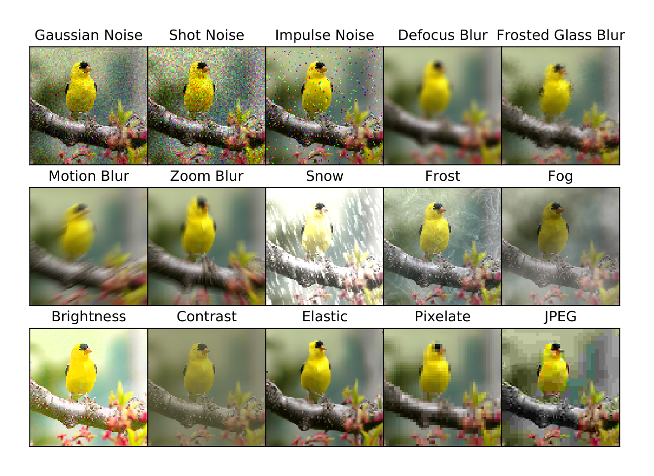
Hendrycks & Dietterich (2019) propose to benchmark robustness of object recognition with 15 types of corruptions from four broad categories: noise, blur, weather and digital. Each corruption type comes in five levels of severity, with level 5 the most severe (details and sample images in the appendix). The corruptions are simulated to mimic real-world corruptions as much as possible on copies of the test set for both CIFAR-10 and ImageNet. The new test sets are named as CIFAR-10-C and ImageNet-C, respectively. In the proposed benchmark, training should be done on the original training set, and the diversity of corruption types should make it difficult for any methods to work well across the board if it relies too much on corruption specific knowledge. For online Test-Time Training, we take the entire test set as a stream of incoming images, and update and test on each image in an online manner as it arrives.

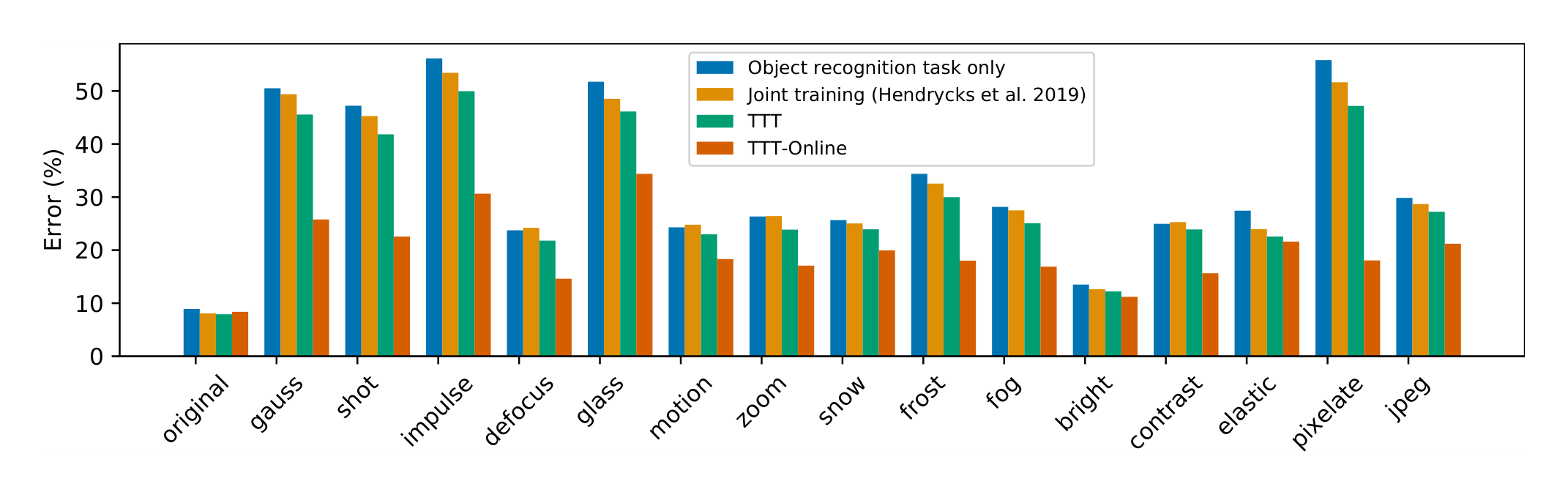
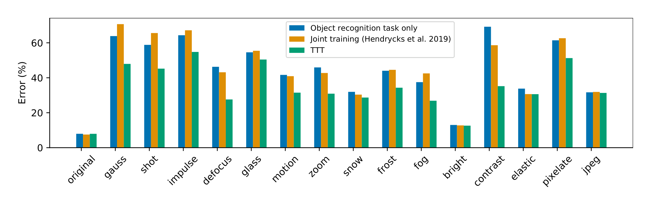
CIFAR-10-C. Our results on the level 5 corruptions (most severe) are shown in Figure 1. The results on levels 1-4 are shown in Section A4 in appendix. Across all five levels and 15 corruption types, both standard and online versions of Test-Time Training improve over the object recognition task only baseline by a large margin. The standard version always improves over joint training, and the online version often improves significantly (>10%) over joint training and never hurts by more than 0.2%. Specifically, TTT-Online contributes >24% on the three noise types and 38% on pixelation. For a learning problem with the seemingly unstable setup that abuses a single image, this kind of consistency is rather surprising.

The baseline ResNet-26 with object recognition task only has error 8.9% on the original test set of CIFAR-10. The joint training baseline actually improves performance on the original to 8.1%. More surprisingly, unlike many other methods that trade off original performance for robustness, Test-Time Training further improves on the original test set by 0.2% consistently over multiple independent trials. This suggests that our method does not choose between specificity and generality.

Separate from our method, it is interesting to note that joint training consistently improves over the single-task baseline, as discovered by Hendrycks et al. (2019a). Hendrycks & Dietterich (2019) have also experimented with various other training methods on this benchmark, and point to Adversarial Logit Pairing (ALP) (Kannan et al., 2018) as the most effective approach. Results of this additional baseline on all levels of CIFAR-10-C are shown in the appendix, along with its implementation details. While surprisingly robust under some of the most severe corruptions (especially the three noise types), ALP incurs a much larger error (by a factor of two) on the original distribution and some corruptions (e.g. all levels of contrast and fog), and hurts performance significantly when the corruptions are not as severe (especially on levels 1-3); this kind of tradeoff is to be expected for methods based on adversarial training.

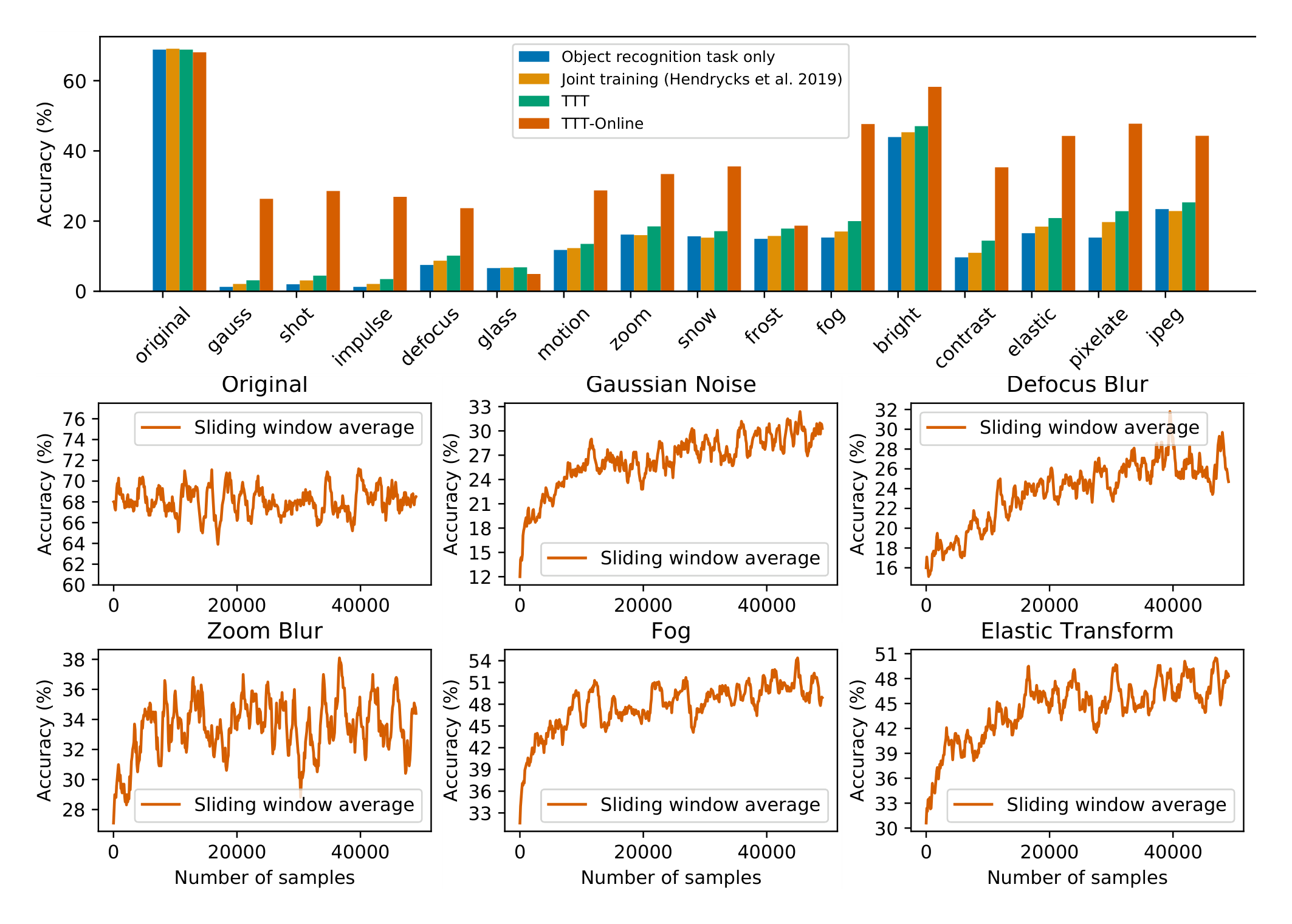
ImageNet-C. Our results on the level 5 corruptions (most severe) are shown in Figure 2. We use accuracy instead of error for this dataset because the baseline performance is very low for most corruptions. The general trend is roughly the same as on CIFAR-10-C. The standard version of TTT always improves over the baseline and joint training, while the online version only hurts on the original by 0.1% over the baseline, but significantly improves (by a factor of more than three) on many of the corruption types.

In the lower panel of Figure 2, we visualize how the accuracy (averaged over a sliding window) of the online version changes as more images are tested. Due to space constraints, we show this plot on the original test set, as well as every third corruption type, following the same order as in the original paper. On the original test set, there is no visible trend in performance change after updating on the 50,000 samples. With corruptions, accuracy has already risen significantly after 10,000 samples, but is still rising towards the end of the 50,000 samples, indicating room for additional improvements if more samples were available. Without seeing a single label, TTT-Online behaves as if we were training on the test set from the appearance of the plots.

: Table 1: Test error (%) on CIFAR-10-C with level 5 corruption. Comparison between online Test-Time Training (TTT-Online) and unsupervised domain adaptation by self-supervision (UDA-SS) (Sun et al., 2019) with access to the entire (unlabeled) test set during training. We highlight the lower error in bold. We have abbreviated the names of the corruptions, in order: original test set, Gaussian noise, shot noise, impulse noise, defocus blur, glass blue, motion blur, zoom blur, snow, frost, fog, brightness, contrast, elastic transformation, pixelation, and JPEG compression. The reported numbers for TTT-Online are the same as in Figure 1. See complete table in Table A2.

\begin{tabular}{c|c|c|c|c|c|c|c|c|c|c|c|c|c|c|c|c}
\hline
& orig & gauss & shot & impul & defoc & glass & motn & zoom & snow & frost & fog & brit & contr & elast & pixel & jpeg \\
\hline
TTT-Online & \textbf{8.2} & \textbf{25.8} & \textbf{22.6} & 30.6 & \textbf{14.6} & \textbf{34.4} & \textbf{18.3} & \textbf{17.1} & \textbf{20.0} & \textbf{18.0} & \textbf{16.9} & \textbf{11.2} & 15.6 & \textbf{21.6} & \textbf{18.1} & \textbf{21.2} \\
\hline
UDA-SS & 9.0 & 28.2 & 26.5 & \textbf{20.8} & 15.6 & 43.7 & 24.5 & 23.8 & 25.0 & 24.9 & 17.2 & 12.7 & \textbf{11.6} & 22.1 & 20.3 & 22.6 \\
\hline
\end{tabular}

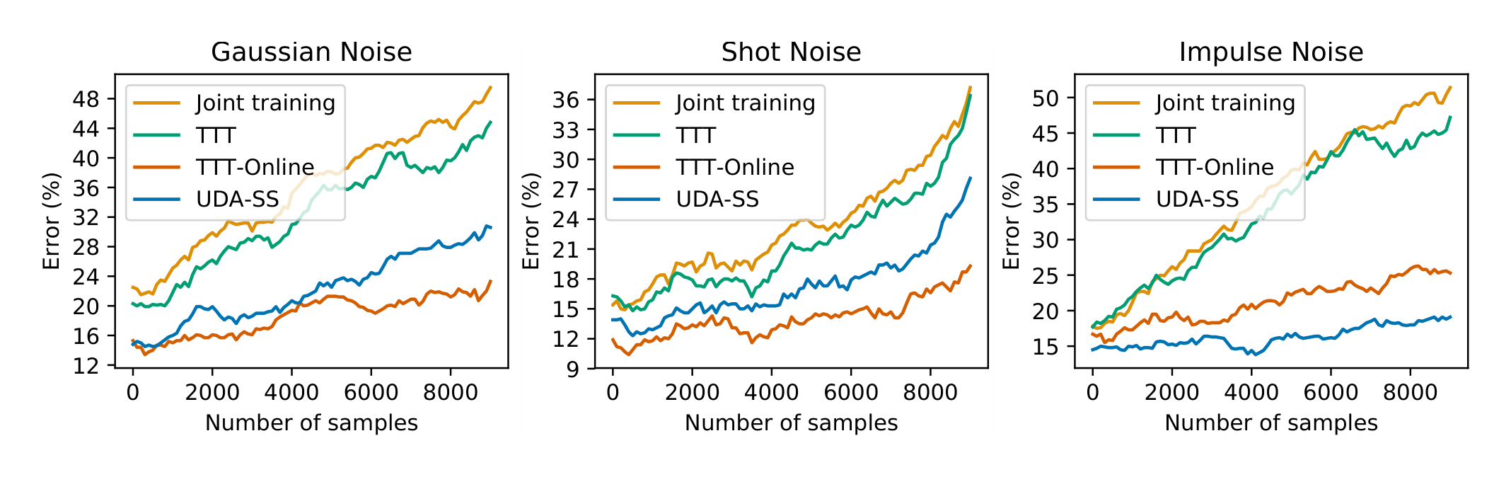
Comparison with unsupervised domain adaptation. Table 1 empirically compares online Test-Time Training (TTT-Online) with unsupervised domain adaptation through self-supervision (UDA-SS) (Sun et al., 2019), which is similar to our method in spirit but is designed for the setting of unsupervised domain adaptation (Section 5 provides a survey of other related work in this setting). Given labeled data from the training distribution and unlabeled data from the test distribution, UDA-SS hopes to find an invariant representation that extracts useful features for both distributions by learning to perform a self-supervised task, specifically rotation prediction, simultaneously on data from both. It then learns a labeling function on top of the invariant representation using the labeled data. In our experiments, the unlabeled data given to UDA-SS is the entire test set itself without the labels.

Because TTT-Online can only learn from the unlabeled test samples that have already been evaluated on, it is given less information than UDA-SS at all times. In this sense, UDA-SS should be regarded as an oracle rather than a baseline. Surprisingly, TTT-Online outperforms UDA-SS on 13 out of the 15 corruptions as well as the original distribution. Our explanation is that UDA-SS has to find an invariant representation for both distributions, while TTT-Online only adapts the representation to be good for the current test distribution. That is, TTT-Online has the flexibility to forget the training distribution representation, which is no longer relevant. This suggests that in our setting, forgetting is not harmful and perhaps should even be taken advantage of.

Gradually changing distribution shifts. In our previous experiments, we have been evaluating the online version under the assumption that the test inputs $x_t$ for $t = 1\ldots n$ are all sampled from the same test distribution $Q$, which can be different from the training distribution $P$. This assumption is indeed satisfied for i.i.d. samples from a shuffled test set. But here we show that this assumption can in fact be relaxed to allow $x_t \sim Q_t$, where $Q_t$ is close to $Q_{t+1}$ (in the sense of distributional distance). We call this the assumption of gradually changing distribution shifts. We perform experiments by simulating such distribution shifts on the three noise types of CIFAR-10-C. For each noise type, $x_t$ is corrupted with standard deviation $\sigma_t$, and $\sigma_1, \ldots, \sigma_n$ interpolate between the standard deviation of level 1 and level 5. So $x_t$ is more severely corrupted as we evaluate further into the test set and $t$ grows larger. As shown in Figure 3, TTT-Online still improves upon joint training (and our standard version) with this relaxed assumption, and even upon UDA-SS for the first two noise types.

: Table 2: Class-wise and average classification accuracy (%) on CIFAR classes in VID-Robust, adapted from (Shankar et al., 2019). Test-Time Training (TTT) and online Test-Time Training (TTT-Online) improve over the two baselines on average, and by a large margin on “ship” and “dog” classes where the rotation task is more meaningful than in classes like “airplane” (sample images in Figure A7).

\begin{tabular}{c|ccccccc|c}
\hline
Accuracy (\%) & Airplane & Bird & Car & Dog & Cat & Horse & Ship & Average \\
\hline
Object recognition task only & 67.9 & 35.8 & 42.6 & 14.7 & 52.0 & 42.0 & 66.7 & \textbf{41.4} \\
\hline
Joint training \scriptsize(Hendrycks et al., 2019a) & 70.2 & 36.7 & 42.6 & 15.5 & 52.0 & 44.0 & 66.7 & \textbf{42.4} \\
\hline
TTT (standard version) & 70.2 & 39.2 & 42.6 & 21.6 & 54.7 & 46.0 & 77.8 & \textbf{45.2} \\
\hline
TTT-Online & 70.2 & 39.2 & 42.6 & 22.4 & 54.7 & 46.0 & 77.8 & \textbf{45.4} \\
\hline
\end{tabular}

3.2. Object Recognition on Video Frames

The Robust ImageNet Video Classification (VID-Robust) dataset was developed by Shankar et al. (2019) from the ImageNet Video detection dataset (Russakovsky et al., 2015), to demonstrate how deep models for object recognition trained on ImageNet (still images) fail to adapt well to video frames. The VID-Robust dataset contains 1109 sets of video frames in 30 classes; each set is a short video clip of frames that are similar to an anchor frame. Our results are reported on the anchor frames. To map the 1000 ImageNet classes to the 30 VID-Robust classes, we use the max-conversion function in Shankar et al. (2019). Without any modifications for videos, we apply our method to VID-Robust on top of the same ImageNet model as in the previous subsection. Our classification accuracy is reported in Table 3.

: Table 3: Test accuracy (%) on VID-Robust dataset (Shankar et al., 2019). TTT and TTT-Online improve over the baselines.

\begin{tabular}{c|c}
\hline
Method & Accuracy (\%) \\
\hline
Object recognition task only & 62.7 \\
\hline
Joint training \scriptsize(Hendrycks et al., 2019a) & 63.5 \\
\hline
TTT (standard version) & 63.8 \\
\hline
TTT-Online & 64.3 \\
\hline
\end{tabular}

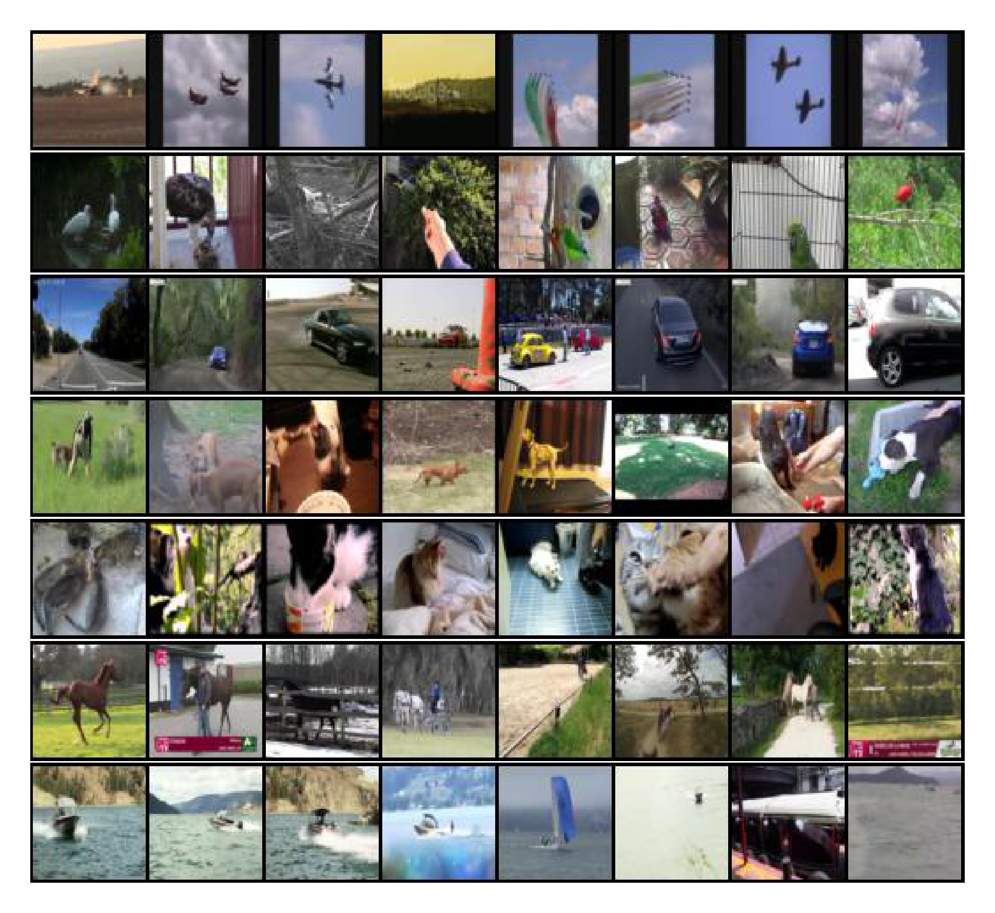
In addition, we take the seven classes in VID-Robust that overlap with CIFAR-10, and re-scale those video frames to the size of CIFAR-10 images, as a new test set for the model trained on CIFAR-10 in the previous subsection. Again, we apply our method to this dataset without any modifications. Our results are shown in Table 2, with a breakdown for each class. Noticing that Test-Time Training does not improve on the airplane class, we inspect some airplane samples (Figure A7), and observe black margins on two sides of most images, which provide a trivial hint for rotation prediction. In addition, given an image of airplanes in the sky, it is often impossible even for humans to tell if it is rotated. This shows that our method requires the self-supervised task to be both well defined and non-trivial.

3.3. CIFAR-10.1: Unknown Distribution Shifts

CIFAR-10.1 (Recht et al., 2018) is a new test set of size 2000 modeled after CIFAR-10, with the exact same classes and image dimensionality, following the dataset creation process documented by the original CIFAR-10 paper as closely as possible. The purpose is to investigate the distribution shifts present between the two test sets, and the effect on object recognition. All models tested by the authors suffer a large performance drop on CIFAR-10.1 comparing to CIFAR-10, even though there is no human noticeable difference, and both have the same human accuracy. This demonstrates how insidious and ubiquitous distribution shifts are, even when researchers strive to minimize them.

: Table 4: Test error (%) on CIFAR-10.1 (Recht et al., 2018). TTT is the first method to improve the performance of an existing model on this new test set.

\begin{tabular}{c|c}
\hline
Method & Error (\%) \\
\hline
Object recognition task only & 17.4 \\
\hline
Joint training \scriptsize(Hendrycks et al., 2019a) & 16.7 \\
\hline
TTT (standard version) & 15.9 \\
\hline
\end{tabular}

The distribution shifts from CIFAR-10 to CIFAR-10.1 pose an extremely difficult problem, and no prior work has been able to improve the performance of an existing model on this new test set, probably because: 1) researchers cannot even identify the distribution shifts, let alone describe them mathematically; 2) the samples in CIFAR-10.1 are only revealed at test time; and even if they were revealed during training, the distribution shifts are too subtle, and the sample size is too small, for domain adaptation (Recht et al., 2018).

On the original CIFAR-10 test set, the baseline with only object recognition has error 8.9%, and with joint training has 8.1%; comparing to the first two rows of Table 4, both suffer the typical performance drop (by a factor of two). TTT yields an improvement of 0.8% (relative improvement of 4.8%) over joint training. We recognize that this improvement is small relative to the performance drop, but see it as an encouraging first step for this very difficult problem.

$Figure 4. Scatter plot of the inner product between the gradients (on the shared feature extractor $\theta_e$) of the main task $l_m$ and the self-supervised task $l_s$, and the improvement in test error (%) from Test-Time Training, for the standard (left) and online (right) version. Each point is the average over a test set, and each scatter plot has 75 test sets, from all 15 types of corruptions over five levels as described in subsection 3.1. The blue lines and bands are the best linear fits and the 99% confidence intervals. The linear correlation coefficients are 0.93 and 0.89 respectively, indicating strong positive correlation between the two quantities, as suggested by Theorem 1.$

4. Theoretical Results

Section Summary: This section presents a preliminary theoretical analysis of when Test-Time Training succeeds, showing that positive correlation between the gradients of the main task loss and the self-supervised loss reliably improves performance on convex models. The authors first demonstrate the idea with a simple two-layer linear regression toy model, where a single gradient step on the auxiliary loss can drive the main loss to zero provided the gradients point in similar directions. They then prove a general result for smooth convex losses and confirm through experiments that the same gradient-correlation principle strongly predicts gains even for the non-convex deep networks used in their earlier sections.

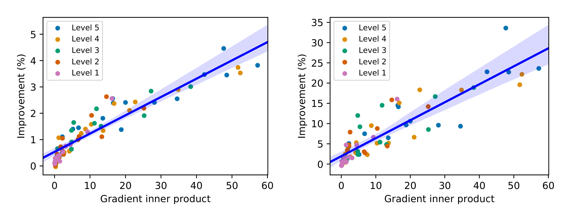
This section contains our preliminary study of when and why Test-Time Training is expected to work. For convex models, we prove that positive gradient correlation between the loss functions leads to better performance on the main task after Test-Time Training. Equipped with this insight, we then empirically demonstrate that gradient correlation governs the success of Test-Time Training on the deep learning model discussed in Section 3.

Before stating our main theoretical result, we first illustrate the general intuition with a toy model. Consider a regression problem where $x \in \mathbb{R}^d$ denotes the input, $y_1 \in \mathbb{R}$ denotes the label, and the objective is the square loss $(\hat{y} - y_1)^2/2$ for a prediction $\hat{y}$. Consider a two layer linear network parametrized by $A \in \mathbb{R}^{h \times d}$ and $v \in \mathbb{R}^h$ (where $h$ stands for the hidden dimension). The prediction according to this model is $\hat{y} = v^\top A x$, and the main task loss is

$ l_m(x, y_1; A, v) = \frac{1}{2}\left(y_1 - v^\top A x\right)^2.\tag{4} $

In addition, consider a self-supervised regression task that also uses the square loss and automatically generates a label $y_2$ for $x$. Let the self-supervised head be parametrized by $w \in \mathbb{R}^h$. Then the self-supervised task loss is

$ l_s(x, y_2; A, w) = \frac{1}{2}\left(y_2 - w^\top A x\right)^2.\tag{5} $

Now we apply Test-Time Training to update the shared feature extractor $A$ by one step of gradient descent on $l_s$, which we can compute with $y_2$ known. This gives us

$ A' \leftarrow A - \eta \left(y_2 - w^\top A x\right)\left(-w x^\top\right),\tag{6} $

where $A'$ is the updated matrix and $\eta$ is the learning rate. If we set $\eta = \eta^*$ where

$ \eta^* = \frac{y_1 - v^\top A x}{\left(y_2 - w^\top A x\right) v^\top w x^\top x},\tag{7} $

then with some simple algebra, it is easy to see that the main task loss $l_m(x, y_1; A', v) = 0$. Concretely, Test-Time Training drives the main task loss down to zero with a single gradient step for a carefully chosen learning rate. In practice, this learning rate is unknown since it depends on the unknown $y_1$. However, since our model is convex, as long as $\eta^*$ is positive, it suffices to set $\eta$ to be a small positive constant (see details in the appendix). If $x \neq 0$, one sufficient condition for $\eta^*$ to be positive (when neither loss is zero) is to have

$ \text{sign}\left(y_1 - v^\top A x\right) = \text{sign}\left(y_2 - w^\top A x\right)\tag{8} $

$ \text{and } v^\top w > 0.\tag{9} $

For our toy model, both parts of the condition above have an intuition interpretation. The first part says that the mistakes should be correlated, in the sense that predictions from both tasks are mistaken in the same direction. The second part, $v^\top w > 0$, says that the decision boundaries on the feature space should be correlated. In fact, these two parts hold iff. $\langle \nabla l_m(A), \nabla l_s(A) \rangle > 0$ (see a simple proof of this fact in the appendix). To summarize, if the gradients have positive correlation, Test-Time Training is guaranteed to reduce the main task loss. Our main theoretical result extends this to general smooth and convex loss functions.

Theorem 1. Let $l_m(x, y; \theta)$ denote the main task loss on test instance $x, y$ with parameters $\theta$, and $l_s(x; \theta)$ the self-supervised task loss that only depends on $x$. Assume that for all $x, y$, $l_m(x, y; \theta)$ is differentiable, convex and $\beta$-smooth in $\theta$, and both $|\nabla l_m(x, y; \theta)|, |\nabla l_s(x, \theta)| \le G$ for all $\theta$. With a fixed learning rate $\eta = \frac{\epsilon}{\beta G^2}$, for every $x, y$ such that

$ \langle \nabla l_m(x, y; \theta), \nabla l_s(x; \theta) \rangle > \epsilon,\tag{10} $

we have

$ l_m(x, y; \theta) > l_m(x, y; \theta(x)),\tag{11} $

where $\theta(x) = \theta - \eta \nabla l_s(x; \theta)$ i.e. Test-Time Training with one step of gradient descent.

The proof uses standard techniques in optimization, and is left for the appendix. Theorem 1 reveals gradient correlation as a determining factor of the success of Test-Time Training in the smooth and convex case. In Figure 4, we empirically show that our insight also holds for non-convex loss functions, on the deep learning model and across the diverse set of corruptions considered in Section 3; stronger gradient correlation clearly indicates more performance improvement over the baseline.

5. Related Work

Section Summary: This section reviews prior research on adapting models at test time by leveraging the input data itself, such as through upsampling tricks, online student-teacher updates, or bootstrapping from easy examples in an image. It also covers self-supervised learning methods that generate their own training signals from data via tasks like rotation prediction, along with efforts to improve robustness against both adversarial attacks and natural corruptions or distribution shifts. Finally, it discusses unsupervised domain adaptation and domain generalization approaches that handle shifts between training and test data, noting how test-time training builds on but differs from these by avoiding the need to anticipate specific target distributions in advance.

Learning on test instances. Shocher et al. (2018) provide a key inspiration for our work by showing that image super-resolution could be learned at test time simply by trying to upsample a downsampled version of the input image. More recently, Bau et al. (2019) improve photo manipulation by adapting a pre-trained GAN to the statistics of the input image. One of the earlier examples of this idea comes from Jain & Learned-Miller (2011), who improve Viola-Jones face detection (Viola et al., 2001) by bootstrapping the more difficult faces in an image from the more easily detected faces in that same image. The online version of our algorithm is inspired by the work of Mullapudi et al. (2018), which makes video segmentation more efficient by using a student model that learns online from a teacher model. The idea of online updates has also been used in Kalal et al. (2011) for tracking and detection. A recent work in echocardiography (Zhu et al., 2019) improves the deep learning model that tracks myocardial motion and cardiac blood flow with sequential updates. Lastly, we share the philosophy of transductive learning (Vapnik, 2013; Gammerman et al., 1998), but have little in common with their classical algorithms; recent work by Tripuraneni & Mackey (2019) theoretically explores this for linear prediction, in the context of debiasing the LASSO estimator.

Self-supervised learning studies how to create labels from the data, by designing various pretext tasks that can learn semantic information without human annotations, such as context prediction (Doersch et al., 2015), solving jigsaw puzzles (Noroozi & Favaro, 2016), colorization (Larsson et al., 2017; Zhang et al., 2016), noise prediction (Bojanowski & Joulin, 2017), feature clustering (Caron et al., 2018). Our paper uses rotation prediction (Gidaris et al., 2018). Asano et al. (2019) show that self-supervised learning on only a single image, surprisingly, can produce low-level features that generalize well. Closely related to our work, Hendrycks et al. (2019a) propose that jointly training a main task and a self-supervised task (our joint training baseline in Section 3) can improve robustness on the main task. The same idea is used in few-shot learning (Su et al., 2019), domain generalization (Carlucci et al., 2019), and unsupervised domain adaptation (Sun et al., 2019).

Adversarial robustness studies the robust risk $R_{P,\Delta}(\theta) = \mathbb{E}{x,y \sim P} \max{\delta \in \Delta} l(x + \delta, y; \theta)$, where $l$ is some loss function, and $\Delta$ is the set of perturbations; $\Delta$ is often chosen as the $L_p$ ball, for $p \in {1, 2, \infty}$. Many popular algorithms formulate and solve this as a robust optimization problem (Goodfellow et al., 2014; Madry et al., 2017; Sinha et al., 2017; Raghunathan et al., 2018; Wong & Kolter, 2017; Croce et al., 2018), and the most well known technique is adversarial training. Another line of work is based on randomized smoothing (Cohen et al., 2019; Salman et al., 2019), while some other approaches, such as input transformations (Guo et al., 2017; Song et al., 2017), are shown to be less effective (Athalye et al., 2018). There are two main problems with the approaches above. First, all of them can be seen as smoothing the decision boundary. This establishes a theoretical tradeoff between accuracy and robustness (Tsipras et al., 2018; Zhang et al., 2019), which we also observe empirically with our adversarial training baseline in Section 3. Intuitively, the more diverse $\Delta$ is, the less effective this one-boundary-fits-all approach can be for a particular element of $\Delta$. Second, adversarial methods rely heavily on the mathematical structure of $\Delta$, which might not accurately model perturbations in the real world. Therefore, generalization remains hard outside of the $\Delta$ we know in advance or can mathematically model, especially for non-adversarial distribution shifts. Empirically, Kang et al. (2019) shows that robustness for one $\Delta$ might not transfer to another, and training on the $L_\infty$ ball actually hurts robustness on the $L_1$ ball.

Non-adversarial robustness studies the effect of corruptions, perturbations, out-of-distribution examples, and real-world distribution shifts (Hendrycks et al., 2019b;a; 2018; Hendrycks & Gimpel, 2016). Geirhos et al. (2018) show that training on images corrupted by Gaussian noise makes deep learning models robust to this particular noise type, but does not improve performance on images corrupted by another noise type e.g. salt-and-pepper noise.

Unsupervised domain adaptation (a.k.a. transfer learning) studies the problem of distribution shifts, when an unlabeled dataset from the test distribution (target domain) is available at training time, in addition to a labeled dataset from the training distribution (source domain) (Chen et al., 2011; Gong et al., 2012; Long et al., 2015; Ganin et al., 2016; Long et al., 2016; Tzeng et al., 2017; Hoffman et al., 2017; Csurka, 2017; Chen et al., 2018). The limitation of the problem setting, however, is that generalization might only be improved for this specific test distribution, which can be difficult to anticipate in advance. Prior work try to anticipate broader distributions by using multiple and evolving domains (Hoffman et al., 2018; 2012; 2014). Test-Time Training does not anticipate any test distribution, by changing the setting of unsupervised domain adaptation, while taking inspiration from its algorithms. Our paper is a follow-up to Sun et al. (2019), which we explain and empirically compare with in Section 3. Our update rule can be viewed as performing one-sample unsupervised domain adaptation on the fly, with the caveat that standard domain adaptation techniques might become ill-defined when there is only one sample from the target domain.

Domain generalization studies the setting where a meta distribution generates multiple environment distributions, some of which are available during training (source), while others are used for testing (target) (Li et al., 2018; Shankar et al., 2018; Muandet et al., 2013; Balaji et al., 2018; Ghifary et al., 2015; Motiian et al., 2017; Li et al., 2017a; Gan et al., 2016). With only a few environments, information on the meta distribution is often too scarce to be helpful, and with many environments, we are back to the i.i.d. setting where each environment can be seen as a sample, and a strong baseline is to simply train on all the environments (Li et al., 2019). The setting of domain generalization is limited by the inherent tradeoff between specificity and generality of a fixed decision boundary, and the fact that generalization is again elusive outside of the meta distribution i.e. the actual $P$ learned by the algorithm.

One (few)-shot learning studies how to learn a new task or a new classification category using only one (or a few) sample(s), on top of a general representation that has been learned on diverse samples (Snell et al., 2017; Vinyals et al., 2016; Fei-Fei et al., 2006; Ravi & Larochelle, 2016; Li et al., 2017b; Finn et al., 2017; Gidaris & Komodakis, 2018). Our update rule can be viewed as performing one-shot self-supervised learning and can potentially be improved by progress in one-shot learning.

Continual learning (a.k.a. learning without forgetting) studies the setting where a model is made to learn a sequence of tasks, and not forget about the earlier ones while training for the later (Li & Hoiem, 2017; Lopez-Paz & Ranzato, 2017; Kirkpatrick et al., 2017; Santoro et al., 2016). In contrast, with Test-Time Training, we are not concerned about forgetting the past test samples since they have already been evaluated on; and if a past sample comes up by any chance, it would go through Test-Time Training again. In addition, the impact of forgetting the training set is minimal, because both tasks have already been jointly trained.

Online learning (a.k.a. online optimization) is a well-studied area of learning theory (Shalev-Shwartz et al., 2012; Hazan et al., 2016). The basic setting repeats the following: receive $x_t$, predict $\hat{y}_t$, receive $y_t$ from a worst-case oracle, and learn. Final performance is evaluated using the regret, which colloquially translates to how much worse the online learning algorithm performs in comparison to the best fixed model in hindsight. In contrast, our setting never reveals any $y_t$ during testing even for the online version, so we do not need to invoke the concept of the worst-case oracle or the regret. Also, due to the lack of feedback from the environment after predicting, our algorithm is motivated to learn (with self-supervision) before predicting $\hat{y}_t$ instead of after. Note that some of the previously covered papers (Hoffman et al., 2014; Jain & Learned-Miller, 2011; Mullapudi et al., 2018) use the term “online learning” outside of the learning theory setting, so the term can be overloaded.

6. Discussion

Section Summary: The discussion notes that test-time training could extend naturally to tasks such as segmentation and detection, as well as to fields like speech recognition and natural language processing, where domain experts might design more effective self-supervised tasks. It also proposes using this approach as a fresh evaluation benchmark for general self-supervised methods beyond the usual pre-training and fine-tuning setups. More broadly, the authors hope their work will encourage abandoning the fixed boundary between training and testing, moving toward models that keep learning after deployment.

The idea of test-time training also makes sense for other tasks, such as segmentation and detection, and in other fields, such as speech recognition and natural language processing. For machine learning practitioners with prior domain knowledge in their respective fields, their expertise can be leveraged to design better special-purpose self-supervised tasks for test-time training. Researchers for general-purpose self-supervised tasks can also use test-time training as an evaluation benchmark, in addition to the currently prevalent benchmark of pre-training and fine-tuning.

More generally, we hope this paper can encourage researchers to abandon the self-imposed constraint of a fixed decision boundary for testing, or even the artificial division between training and testing altogether. Our work is but a small step toward a new paradigm where much of the learning happens after a model is deployed.

Acknowledgements. This work is supported by NSF grant 1764033, DARPA and Berkeley DeepDrive. This paper took a long time to develop, and benefited from conversations with many of our colleagues, including Ben Recht and his students Ludwig Schmidt, Vaishaal Shanker and Becca Roelofs; Ravi Teja Mullapudi, Achal Dave and Deva Ramanan; and Armin Askari, Allan Jabri, Ashish Kumar, Angjoo Kanazawa and Jitendra Malik.

References

Section Summary: The references section presents a lengthy bibliography of academic papers, preprints, and conference proceedings drawn mainly from machine learning and computer vision. These works address topics including domain adaptation and generalization, adversarial robustness of neural networks, unsupervised representation learning, and meta-learning methods, with many appearing in venues such as NeurIPS, CVPR, and ECCV. The citations range from foundational studies of the 1990s through recent technical advances published in 2019.

Asano, Y. M., Rupprecht, C., and Vedaldi, A. Surprising effectiveness of few-image unsupervised feature learning. arXiv preprint arXiv:1904.13132, 2019.

Athalye, A., Carlini, N., and Wagner, D. Obfuscated gradients give a false sense of security: Circumventing defenses to adversarial examples. arXiv preprint arXiv:1802.00420, 2018.

Balaji, Y., Sankaranarayanan, S., and Chellappa, R. Metareg: Towards domain generalization using meta-regularization. In Advances in Neural Information Processing Systems, pp. 998–1008, 2018.

Bau, D., Strobelt, H., Peebles, W., Wulff, J., Zhou, B., Zhu, J.-Y., and Torralba, A. Semantic photo manipulation with a generative image prior. ACM Transactions on Graphics (TOG), 38(4):59, 2019.

Bojanowski, P. and Joulin, A. Unsupervised learning by predicting noise. In Proceedings of the 34th International Conference on Machine Learning-Volume 70, pp. 517–526. JMLR. org, 2017.

Carlucci, F. M., D’Innocente, A., Bucci, S., Caputo, B., and Tommasi, T. Domain generalization by solving jigsaw puzzles. In Proceedings of the IEEE Conference on Computer Vision and Pattern Recognition, pp. 2229–2238, 2019.

Caron, M., Bojanowski, P., Joulin, A., and Douze, M. Deep clustering for unsupervised learning of visual features. In Proceedings of the European Conference on Computer Vision (ECCV), pp. 132–149, 2018.

Caruana, R. Multitask learning. Machine learning, 28(1):41–75, 1997.

Chen, M., Weinberger, K. Q., and Blitzer, J. Co-training for domain adaptation. In Advances in neural information processing systems, pp. 2456–2464, 2011.

Chen, X., Sun, Y., Athiwaratkun, B., Cardie, C., and Weinberger, K. Adversarial deep averaging networks for crosslingual sentiment classification. Transactions of the Association for Computational Linguistics, 6:557–570, 2018.

Cohen, J. M., Rosenfeld, E., and Kolter, J. Z. Certified adversarial robustness via randomized smoothing. arXiv preprint arXiv:1902.02918, 2019.

Croce, F., Andriushchenko, M., and Hein, M. Provable robustness of relu networks via maximization of linear regions. arXiv preprint arXiv:1810.07481, 2018.

Csurka, G. Domain adaptation for visual applications: A comprehensive survey. arXiv preprint arXiv:1702.05374, 2017.

Ding, G. W., Wang, L., and Jin, X. AdverTorch v0.1: An adversarial robustness toolbox based on pytorch. arXiv preprint arXiv:1902.07623, 2019.

Doersch, C., Gupta, A., and Efros, A. A. Unsupervised visual representation learning by context prediction. In Proceedings of the IEEE International Conference on Computer Vision, pp. 1422–1430, 2015.

Fei-Fei, L., Fergus, R., and Perona, P. One-shot learning of object categories. IEEE transactions on pattern analysis and machine intelligence, 28(4):594–611, 2006.

Finn, C., Abbeel, P., and Levine, S. Model-agnostic meta-learning for fast adaptation of deep networks. In Proceedings of the 34th International Conference on Machine Learning-Volume 70, pp. 1126–1135. JMLR. org, 2017.

Gammerman, A., Vovk, V., and Vapnik, V. Learning by transduction. In Proceedings of the Fourteenth conference on Uncertainty in artificial intelligence, pp. 148–155. Morgan Kaufmann Publishers Inc., 1998.

Gan, C., Yang, T., and Gong, B. Learning attributes equals multi-source domain generalization. In Proceedings of the IEEE Conference on Computer Vision and Pattern Recognition, pp. 87–97, 2016.

Ganin, Y., Ustinova, E., Ajakan, H., Germain, P., Larochelle, H., Laviolette, F., Marchand, M., and Lempitsky, V. Domain-adversarial training of neural networks. The Journal of Machine Learning Research, 17(1):2096–2030, 2016.

Geirhos, R., Temme, C. R., Rauber, J., Schütt, H. H., Bethge, M., and Wichmann, F. A. Generalisation in humans and deep neural networks. In Advances in Neural Information Processing Systems, pp. 7538–7550, 2018.

Ghifary, M., Bastiaan Kleijn, W., Zhang, M., and Balduzzi, D. Domain generalization for object recognition with multi-task autoencoders. In Proceedings of the IEEE international conference on computer vision, pp. 2551–2559, 2015.

Gidaris, S. and Komodakis, N. Dynamic few-shot visual learning without forgetting. In Proceedings of the IEEE Conference on Computer Vision and Pattern Recognition, pp. 4367–4375, 2018.

Gidaris, S., Singh, P., and Komodakis, N. Unsupervised representation learning by predicting image rotations. arXiv preprint arXiv:1803.07728, 2018.

Gong, B., Shi, Y., Sha, F., and Grauman, K. Geodesic flow kernel for unsupervised domain adaptation. In 2012 IEEE Conference on Computer Vision and Pattern Recognition, pp. 2066–2073. IEEE, 2012.

Goodfellow, I. J., Shlens, J., and Szegedy, C. Explaining and harnessing adversarial examples. arXiv preprint arXiv:1412.6572, 2014.

Guo, C., Rana, M., Cisse, M., and van der Maaten, L. Countering adversarial images using input transformations. arXiv preprint arXiv:1711.00117, 2017.

Hazan, E. et al. Introduction to online convex optimization. Foundations and Trends® in Optimization, 2(3-4):157–325, 2016.

He, K., Zhang, X., Ren, S., and Sun, J. Deep residual learning for image recognition. In Proceedings of the IEEE conference on computer vision and pattern recognition, pp. 770–778, 2016a.

He, K., Zhang, X., Ren, S., and Sun, J. Identity mappings in deep residual networks. In European conference on computer vision, pp. 630–645. Springer, 2016b.

He, K., Girshick, R., and Dollár, P. Rethinking imagenet pre-training. arXiv preprint arXiv:1811.08883, 2018.

Hendrycks, D. and Dietterich, T. Benchmarking neural network robustness to common corruptions and perturbations. arXiv preprint arXiv:1903.12261, 2019.

Hendrycks, D. and Gimpel, K. A baseline for detecting misclassified and out-of-distribution examples in neural networks. arXiv preprint arXiv:1610.02136, 2016.

Hendrycks, D., Mazeika, M., Wilson, D., and Gimpel, K. Using trusted data to train deep networks on labels corrupted by severe noise. In Advances in neural information processing systems, pp. 10456–10465, 2018.

Hendrycks, D., Lee, K., and Mazeika, M. Using pre-training can improve model robustness and uncertainty. arXiv preprint arXiv:1901.09960, 2019a.

Hendrycks, D., Mazeika, M., Kadavath, S., and Song, D. Improving model robustness and uncertainty estimates with self-supervised learning. arXiv preprint, 2019b.

Hoffman, J., Kulis, B., Darrell, T., and Saenko, K. Discovering latent domains for multisource domain adaptation. In European Conference on Computer Vision, pp. 702–715. Springer, 2012.

Hoffman, J., Darrell, T., and Saenko, K. Continuous manifold based adaptation for evolving visual domains. In Proceedings of the IEEE Conference on Computer Vision and Pattern Recognition, pp. 867–874, 2014.

Hoffman, J., Tzeng, E., Park, T., Zhu, J.-Y., Isola, P., Saenko, K., Efros, A. A., and Darrell, T. Cycada: Cycle-consistent adversarial domain adaptation. arXiv preprint arXiv:1711.03213, 2017.

Hoffman, J., Mohri, M., and Zhang, N. Algorithms and theory for multiple-source adaptation. In Advances in Neural Information Processing Systems, pp. 8246–8256, 2018.

Huang, G., Sun, Y., Liu, Z., Sedra, D., and Weinberger, K. Q. Deep networks with stochastic depth. In European conference on computer vision, pp. 646–661. Springer, 2016.

Ioffe, S. and Szegedy, C. Batch normalization: Accelerating deep network training by reducing internal covariate shift. arXiv preprint arXiv:1502.03167, 2015.

Jain, V. and Learned-Miller, E. Online domain adaptation of a pre-trained cascade of classifiers. In CVPR 2011, pp. 577–584. IEEE, 2011.

Kalal, Z., Mikolajczyk, K., and Matas, J. Tracking-learning-detection. IEEE transactions on pattern analysis and machine intelligence, 34(7):1409–1422, 2011.

Kang, D., Sun, Y., Brown, T., Hendrycks, D., and Steinhardt, J. Transfer of adversarial robustness between perturbation types. arXiv preprint arXiv:1905.01034, 2019.

Kannan, H., Kurakin, A., and Goodfellow, I. Adversarial logit pairing. arXiv preprint arXiv:1803.06373, 2018.

Kirkpatrick, J., Pascanu, R., Rabinowitz, N., Veness, J., Desjardins, G., Rusu, A. A., Milan, K., Quan, J., Ramalho, T., Grabska-Barwinska, A., et al. Overcoming catastrophic forgetting in neural networks. Proceedings of the national academy of sciences, 114(13):3521–3526, 2017.

Krizhevsky, A. and Hinton, G. Learning multiple layers of features from tiny images. Technical report, Citeseer, 2009.

Larsson, G., Maire, M., and Shakhnarovich, G. Colorization as a proxy task for visual understanding. In CVPR, 2017.

Li, D., Yang, Y., Song, Y.-Z., and Hospedales, T. M. Deeper, broader and artier domain generalization. In Proceedings of the IEEE International Conference on Computer Vision, pp. 5542–5550, 2017a.

Li, D., Zhang, J., Yang, Y., Liu, C., Song, Y.-Z., and Hospedales, T. M. Episodic training for domain generalization. arXiv preprint arXiv:1902.00113, 2019.

Li, Y., Tian, X., Gong, M., Liu, Y., Liu, T., Zhang, K., and Tao, D. Deep domain generalization via conditional invariant adversarial networks. In Proceedings of the European Conference on Computer Vision (ECCV), pp. 624–639, 2018.

Li, Z. and Hoiem, D. Learning without forgetting. IEEE transactions on pattern analysis and machine intelligence, 40(12):2935–2947, 2017.

Li, Z., Zhou, F., Chen, F., and Li, H. Meta-sgd: Learning to learn quickly for few-shot learning. arXiv preprint arXiv:1707.09835, 2017b.

Liu, Z., Sun, M., Zhou, T., Huang, G., and Darrell, T. Rethinking the value of network pruning. arXiv preprint arXiv:1810.05270, 2018.

Long, M., Cao, Y., Wang, J., and Jordan, M. I. Learning transferable features with deep adaptation networks. arXiv preprint arXiv:1502.02791, 2015.

Long, M., Zhu, H., Wang, J., and Jordan, M. I. Unsupervised domain adaptation with residual transfer networks. In Advances in Neural Information Processing Systems, pp. 136–144, 2016.

Lopez-Paz, D. and Ranzato, M. Gradient episodic memory for continual learning. In Advances in Neural Information Processing Systems, pp. 6467–6476, 2017.

Madry, A., Makelov, A., Schmidt, L., Tsipras, D., and Vladu, A. Towards deep learning models resistant to adversarial attacks. arXiv preprint arXiv:1706.06083, 2017.

Motiian, S., Piccirilli, M., Adjeroh, D. A., and Doretto, G. Unified deep supervised domain adaptation and generalization. In Proceedings of the IEEE International Conference on Computer Vision, pp. 5715–5725, 2017.

Muandet, K., Balduzzi, D., and Schölkopf, B. Domain generalization via invariant feature representation. In International Conference on Machine Learning, pp. 10–18, 2013.

Mullapudi, R. T., Chen, S., Zhang, K., Ramanan, D., and Fatahalian, K. Online model distillation for efficient video inference. arXiv preprint arXiv:1812.02699, 2018.

Noroozi, M. and Favaro, P. Unsupervised learning of visual representations by solving jigsaw puzzles. In European Conference on Computer Vision, pp. 69–84. Springer, 2016.

Raghunathan, A., Steinhardt, J., and Liang, P. Certified defenses against adversarial examples. arXiv preprint arXiv:1801.09344, 2018.

Ravi, S. and Larochelle, H. Optimization as a model for few-shot learning. IEEE transactions on pattern analysis and machine intelligence, 2016.

Recht, B., Roelofs, R., Schmidt, L., and Shankar, V. Do cifar-10 classifiers generalize to cifar-10? arXiv preprint arXiv:1806.00451, 2018.

Russakovsky, O., Deng, J., Su, H., Krause, J., Satheesh, S., Ma, S., Huang, Z., Karpathy, A., Khosla, A., Bernstein, M., Berg, A. C., and Fei-Fei, L. ImageNet Large Scale Visual Recognition Challenge. International Journal of Computer Vision (IJCV), 115(3):211–252, 2015. doi: 10.1007/s11263-015-0816-y.

Salman, H., Yang, G., Li, J., Zhang, P., Zhang, H., Razenshteyn, I., and Bubeck, S. Provably robust deep learning via adversarially trained smoothed classifiers. arXiv preprint arXiv:1906.04584, 2019.

Santoro, A., Bartunov, S., Botvinick, M., Wierstra, D., and Lillicrap, T. Meta-learning with memory-augmented neural networks. In International conference on machine learning, pp. 1842–1850, 2016.

Shalev-Shwartz, S. et al. Online learning and online convex optimization. Foundations and Trends® in Machine Learning, 4(2):107–194, 2012.

Shankar, S., Piratla, V., Chakrabarti, S., Chaudhuri, S., Jyothi, P., and Sarawagi, S. Generalizing across domains via cross-gradient training. arXiv preprint arXiv:1804.10745, 2018.

Shankar, V., Dave, A., Roelofs, R., Ramanan, D., Recht, B., and Schmidt, L. Do image classifiers generalize across time? arXiv, 2019.

Shocher, A., Cohen, N., and Irani, M. zero-shot super-resolution using deep internal learning. In Proceedings of the IEEE Conference on Computer Vision and Pattern Recognition, pp. 3118–3126, 2018.

Sinha, A., Namkoong, H., and Duchi, J. Certifying some distributional robustness with principled adversarial training. arXiv preprint arXiv:1710.10571, 2017.

Snell, J., Swersky, K., and Zemel, R. Prototypical networks for few-shot learning. In Advances in Neural Information Processing Systems, pp. 4077–4087, 2017.

Song, Y., Kim, T., Nowozin, S., Ermon, S., and Kushman, N. Pixeldefend: Leveraging generative models to understand and defend against adversarial examples. arXiv preprint arXiv:1710.10766, 2017.

Su, J.-C., Maji, S., and Hariharan, B. Boosting supervision with self-supervision for few-shot learning. arXiv preprint arXiv:1906.07079, 2019.

Sun, Y., Tzeng, E., Darrell, T., and Efros, A. A. Unsupervised domain adaptation through self-supervision. arXiv preprint, 2019.

Tripuraneni, N. and Mackey, L. Debiasing linear prediction. arXiv preprint arXiv:1908.02341, 2019.

Tsipras, D., Santurkar, S., Engstrom, L., Turner, A., and Madry, A. Robustness may be at odds with accuracy. arXiv preprint arXiv:1805.12152, 2018.

Tzeng, E., Hoffman, J., Saenko, K., and Darrell, T. Adversarial discriminative domain adaptation. In Proceedings of the IEEE Conference on Computer Vision and Pattern Recognition, pp. 7167–7176, 2017.

Vapnik, V. The nature of statistical learning theory. Springer science & business media, 2013.

Vinyals, O., Blundell, C., Lillicrap, T., Wierstra, D., et al. Matching networks for one shot learning. In Advances in neural information processing systems, pp. 3630–3638, 2016.

Viola, P., Jones, M., et al. Rapid object detection using a boosted cascade of simple features. CVPR (1), 1(511-518):3, 2001.

Wong, E. and Kolter, J. Z. Provable defenses against adversarial examples via the convex outer adversarial polytope. arXiv preprint arXiv:1711.00851, 2017.

Zhang, H., Yu, Y., Jiao, J., Xing, E. P., Ghaoui, L. E., and Jordan, M. I. Theoretically principled trade-off between robustness and accuracy. arXiv preprint arXiv:1901.08573, 2019.

Zhang, R., Isola, P., and Efros, A. A. Colorful image colorization. In European conference on computer vision, pp. 649–666. Springer, 2016.

Zhu, W., Huang, Y., Vannan, M. A., Liu, S., Xu, D., Fan, W., Qian, Z., and Xie, X. Neural multi-scale self-supervised registration for echocardiogram dense tracking. arXiv preprint arXiv:1906.07357, 2019.

Appendix: Test-Time Training with Self-Supervision for Generalization under Distribution Shifts

Section Summary: This appendix explores supporting ideas behind test-time training with self-supervision for handling distribution shifts. It first clarifies how the method creates an input-dependent, variable decision boundary rather than a single fixed one, noting why this differs from standard learning theory and avoids needing impractically large models. It then discusses the added computational cost during testing and offers practical ways to speed it up, followed by formal proofs of the theoretical results on a simplified toy problem.

A1. Informal Discussion on Our Variable Decision Boundary

In the introduction, we claim that in traditional supervised learning $\theta$ gives a fixed decision boundary, while our $\theta$ gives a variable decision boundary. Here we informally discuss this claim.

Denote the input space $\mathcal{X}$ and output space $\mathcal{Y}$. A decision boundary is simply a mapping $f : \mathcal{X} \rightarrow \mathcal{Y}$. Let $\Theta$ be a model class e.g $\mathbb{R}^d$. Now consider a family of parametrized functions $g_\theta : \mathcal{X} \rightarrow \mathcal{Y}$, where $\theta \in \Theta$. In the context of deep learning, $g$ is the neural network architecture and $\theta$ contains the parameters. We say that $f$ is a fixed decision boundary w.r.t. $g$ and $\Theta$ if there exists $\theta \in \Theta$ s.t. $f(x) = g_\theta(x)$ for every $x \in \mathcal{X}$, and a variable decision boundary if for every $x \in \mathcal{X}$, there exists $\theta \in \Theta$ s.t. $f(x) = g_\theta(x)$. Note how selection of $\theta$ can depend on $x$ for a variable decision boundary, and cannot for a fixed one. It is then trivial to verify that our claim is true under those definitions.

A critical reader might say that with an arbitrarily large model class, can’t every decision boundary be fixed? Yes, but this is not the end of the story. Let $d = \dim(\mathcal{X}) \times \dim(\mathcal{Y})$, and consider the enormous model class $\Theta' = \mathbb{R}^d$ which is capable of representing all possible mappings between $\mathcal{X}$ and $\mathcal{Y}$. Let $g'_{\theta'}$ simply be the mapping represented by $\theta' \in \Theta'$. A variable decision boundary w.r.t. $g$ and $\Theta$ then indeed must be a fixed decision boundary w.r.t. $g'$ and $\Theta'$, but we would like to note two things. First, without any prior knowledge, generalization in $\Theta'$ is impossible with any finite amount of training data; reasoning about $g'$ and $\Theta'$ is most likely not productive from an algorithmic point of view, and the concept of a variable decision boundary is to avoid such reasoning. Second, selecting $\theta$ based on $x$ for a variable decision boundary can be thought of as “training” on all points $x \in \mathbb{R}^d$; however, “training” only happens when necessary, for the $x$ that it actually encounters.

Altogether, the concept of a variable decision boundary is different from what can be described by traditional learning theory. A formal discussion is beyond the scope of this paper and might be of interest to future work.

A2. Computational Aspects of Our Method

At test time, our method is $2 \times \text{batch_size} \times \text{number_of_iterations}$ times slower than regular testing, which only performs a single forward pass for each sample. As the first work on Test-Time Training, this paper is not as concerned about computational efficiency as improving robustness, but here we provide two potential solutions that might be useful, but have not been thoroughly verified. The first is to use the thresholding trick on $l_s$, introduced as a solution for the small batches problem in the method section. For the models considered in our experiments, roughly 80% of the test instances fall below the threshold, so Test-Time Training can only be performed on the other 20% without much effect on performance, because those 20% contain most of the samples with wrong predictions. The second is to reduce the $\text{number_of_iterations}$ of test-time updates. For the online version, the $\text{number_of_iterations}$ is already 1, so there is nothing to do. For the standard version, we have done some preliminary experiments setting $\text{number_of_iterations}$ to 1 (instead of 10) and learning rate to 0.01 (instead of 0.001), and observing results almost as good as the standard hyper-parameter setting. A more in depth discussion on efficiency is left for future works, which might, during training, explicitly make the model amenable to fast updates.

A3. Proofs

Here we prove the theoretical results in the main paper.

A3.1. The Toy Problem

The following setting applies to the two lemmas; this is simply the setting of our toy problem, reproduced here for ease of reference. Consider a two layer linear network parametrized by $A \in \mathbb{R}^{h \times d}$ (shared) and $v, w \in \mathbb{R}^h$ (fixed) for the two heads, respectively. Denote $x \in \mathbb{R}^d$ the input and $y_1, y_2 \in \mathbb{R}$ the labels for the two tasks, respectively. For the main task loss

$ l_m(A; v) = \frac{1}{2}\left(y_1 - v^\top A x\right)^2,\tag{12} $

and the self-supervised task loss

$ l_s(A; w) = \frac{1}{2}\left(y_2 - w^\top A x\right)^2,\tag{13} $

Test-Time Training yields an updated matrix

$ A' \leftarrow A - \eta \left(y_2 - w^\top A x\right)\left(-w x^\top\right),\tag{14} $

where $\eta$ is the learning rate.

Lemma 1. Following the exposition of the main paper, let

$ \eta^* = \frac{(y_1 - v^\top A x)}{(y_2 - w^\top A x)v^\top w x^\top x}.\tag{15} $

Assume $\eta^ \in [\epsilon, \infty)$ for some $\epsilon > 0$. Then for any $\eta \in (0, \epsilon]$, we are guaranteed an improvement on the main loss i.e. $l_m(A') < l_m(A)$.*

Proof. From the exposition of the main paper, we know that $l_m(A - \eta^* \nabla l_s(A)) = 0$, which can also be derived from simple algebra. Then by convexity, we have

$ l_m\left(A - \eta \nabla l_s(A)\right)\tag{16} $

$ = l_m\left(\left(1 - \frac{\eta}{\eta^*}\right) A + \frac{\eta}{\eta^*} (A - \eta^* \nabla l_s(A))\right)\tag{17} $

$ \le \left(1 - \frac{\eta}{\eta^*}\right) l_m(A) + 0\tag{18} $

$ \le \left(1 - \frac{\eta}{\epsilon}\right) l_m(A)\tag{19} $

$ < l_m(A),\tag{20} $

where the last inequality uses the assumption that $l_m(A) > 0$, which holds because $\eta^* > 0$.

Lemma 2. Define $\langle U, V \rangle = \text{vec}(U)^\top \text{vec}(V)$ i.e. the Frobenious inner product, then

$ \text{sign}(\eta^*) = \text{sign}\left(\langle \nabla l_m(A), \nabla l_s(A) \rangle\right).\tag{21} $

Proof. By simple algebra,

$ \langle \nabla l_m(A), \nabla l_s(A) \rangle $

$ = \left\langle \left(y_1 - v^\top A x\right)\left(-v x^\top\right), \left(y_2 - w^\top A x\right)\left(-w x^\top\right) \right\rangle $

$ = \left(y_1 - v^\top A x\right)\left(y_2 - w^\top A x\right) \text{Tr}\left(x v^\top w x^\top\right) $

$ = \left(y_1 - v^\top A x\right)\left(y_2 - w^\top A x\right) v^\top w x^\top x, $

which has the same sign as $\eta^*$.

A3.2. Proof of Theorem 1

For any $\eta$, by smoothness and convexity,

$ l_m(x, y; \theta(x)) = l_m(x, y; \theta - \eta \nabla l_s(x; \theta)) $

$ \le l_m(x, y; \theta) + \eta \langle \nabla l_m(x, y; \theta), \nabla l_s(x, \theta) \rangle + \frac{\eta^2 \beta}{2} |\nabla l_s(x; \theta)|^2. $

Denote

$ \eta^* = \frac{\langle \nabla l_m(x, y; \theta), \nabla l_s(x, \theta) \rangle}{\beta |\nabla l_s(x; \theta)|^2}. $

Then Equation 22 becomes

$ l_m(x, y; \theta - \eta^* \nabla l_s(x; \theta))\tag{22} $

$ \le l_m(x, y; \theta) - \frac{\langle \nabla l_m(x, y; \theta), \nabla l_s(x, \theta) \rangle^2}{2\beta |\nabla l_s(x; \theta)|^2}.\tag{23} $

And by our assumptions on the gradient norm and gradient inner product,

$ l_m(x, y; \theta) - l_m(x, y; \theta - \eta^* \nabla l_s(x; \theta)) \ge \frac{\epsilon^2}{2\beta G^2}.\tag{24} $

Because we cannot observe $\eta^*$ in practice, we instead use a fixed learning rate $\eta = \frac{\epsilon}{\beta G^2}$, as stated in Theorem 1. Now we argue that this fixed learning rate still improves performance on the main task.

By our assumptions, $\eta^* \ge \frac{\epsilon}{\beta G^2}$, so $\eta \in (0, \eta^*]$. Denote $g = \nabla l_s(x; \theta)$, then by convexity of $l_m$,

$ l_m(x, y; \theta(x)) = l_m(x, y; \theta - \eta g)\tag{25} $

$ = l_m\left(x, y; \left(1 - \frac{\eta}{\eta^*}\right) \theta + \frac{\eta}{\eta^*} (\theta - \eta^* g)\right)\tag{26} $

$ \le \left(1 - \frac{\eta}{\eta^*}\right) l_m(x, y; \theta) + \frac{\eta}{\eta^*} l_m(x, y; \theta - \eta^* g)\tag{27} $

Combining with Equation 24, we have

$ l_m(x, y; \theta(x)) \le \left(1 - \frac{\eta}{\eta^*}\right) l_m(x, y; \theta) + \frac{\eta}{\eta^*} \left(l_m(x, y; \theta) - \frac{\epsilon^2}{2\beta G^2}\right) $

$ = l_m(x, y; \theta) - \frac{\eta}{\eta^*} \frac{\epsilon^2}{2\beta G^2} $

Since $\eta/\eta^* > 0$, we have shown that

$ l_m(x, y; \theta) - l_m(x, y; \theta(x)) > 0.\tag{28} $

A4. Additional Results on the Common Corruptions Dataset

For table aethetics, we use the following abbreviations: B for baseline, JT for joint training, TTT for Test-Time Training standard version, and TTT-Online for online Test-Time Training i.e. the online version.

We have abbreviated the names of the corruptions, in order: original test set, Gaussian noise, shot noise, impulse noise, defocus blur, glass blue, motion blur, zoom blur, snow, frost, fog, brightness, contrast, elastic transformation, pixelation, and JPEG compression.

A4.1. Results Using Batch Normalization

As discussed in the results section, Batch Normalization (BN) is ineffective for small batches, which are the inputs for Test-Time Training (both standard and online version) since there is only one sample available when forming each batch; therefore, our main results are based on a ResNet using Group Normalization (GN). Figure A2 and Table A1 show results of our method on CIFAR-10-C level 5, with a ResNet using Batch Normalization (BN). These results are only meant to be a point of reference for the curious readers.

In the early stage of this project, we have experimented with two potential solutions to the small batches problem with BN. The naive solution is to fix the BN layers during Test-Time Training. but this diminishes the performance gains since there are fewer shared parameters. The better solution, adopted for the results below, is hard example mining: instead of updating on all inputs, we only update on inputs that incur large self-supervised task loss $l_s$, where the large improvements might counter the negative effects of inaccurate statistics.

Test-Time Training (standard version) is still very effective with BN. In fact, some of the improvements are quite dramatic, such as on contrast (34%), defocus blue (18%) and Gaussian noise (22% comparing to joint-training, and 16% comparing to the baseline). Performance on the original distribution is still almost the same, and the original error with BN is in fact slightly lower than with GN, and takes half as many epochs to converge.

We did not further experiment with BN because of two reasons: 1) The online version does not work with BN, because the problem with inaccurate batch statistics is exacerbated when training online for many (e.g. 10000) steps. 2) The baseline error for almost every corruption type is significantly higher with BN than with GN. Although unrelated to the main idea of our paper, we make the interesting note that GN significantly improves model robustness.

A4.2. Additional Baseline: Adversarial Logit Pairing

As discussed in the results section, Hendrycks & Dietterich (2019) point to Adversarial Logit Pairing (ALP) (Kannan et al., 2018) as an effective method for improving model robustness to corruptions and perturbations, even though it was designed to defend against adversarial attacks. We take ALP as an additional baseline on all benchmarks based on CIFAR-10 (using GN), following the training procedure in Kannan et al. (2018) and their recommended hyperparameters. The implementation of the adversarial attack comes from the codebase of Ding et al. (2019). We did not run ALP on ImageNet because the two papers we reference for this method, Kannan et al. (2018) and Hendrycks & Dietterich (2019), did not run on ImageNet or make any claim or recommendation.

A4.3. Results on CIFAR-10-C and ImageNet-C, Level 5

Table A2 and Table A3 correspond to the bar plots in the results section. Two rows of Table A2 have been presented as Table 1 in the main text.

A4.4. Results on CIFAR-10-C, Levels 1-4

The following bar plots and tables are on levels 1-4 of CIFAR-10-C. The original distribution is the same for all levels, so are our results on the original distribution.

A4.5. Direct Comparison with Hendrycks et al. (2019a)

The following comparison has been requested by an anonymous reviewer for our final version. Our joint training baseline is based on Hendrycks et al. (2019a), but also incorporates some architectural changes (see below). We found these changes improved the robustness of our method, and felt that it was important to give the baseline the same benefit. Note that our joint training baseline overall performs better than Hendrycks: Compare Table S2 to Figure 3 of Hendrycks et al. (2019a) (provided by the authors), our baseline has average error of 22.8% across all corruptions and levels, while their average error is 28.6%.

Summary of architectural changes: 1) Group Normalization (GN) instead of Batch Normalization (BN). For completeness, the results with BN are provided in Table S1; c.f. GN results in Table S2 which significantly improves robustness, with or without self-supervision. 2) We split after the second residual group, while they split after the third residual group right before the linear layer. This consistently gives about 0.5% - 1% improvement. 3) We use a ResNet-26, while they use a 40-2 Wide ResNet. But our baseline still performs better than their method even though our network is 4x smaller, due to the two tricks above.

Figure A1. Sample images from the Common Corruptions Benchmark, taken from the original paper by Hendrycks & Dietterich (2019).

Figure A2. Test error (%) on CIFAR-10-C, level 5, ResNet-26 with Batch Normalization.

: Table A1: Test error (%) on CIFAR-10-C, level 5, ResNet-26 with Batch Normalization.

\begin{tabular}{c|c|c|c|c|c|c|c|c|c|c|c|c|c|c|c|c}
\hline
& orig & gauss & shot & impul & defoc & glass & motn & zoom & snow & frost & fog & brit & contr & elast & pixel & jpeg \\
\hline
B & 7.9 & 63.9 & 58.8 & 64.3 & 46.3 & 54.6 & 41.6 & 45.9 & 31.9 & 44.0 & 37.5 & 13.0 & 69.2 & 33.8 & 61.4 & 31.7 \\
\hline
JT & 7.5 & 70.7 & 65.6 & 67.2 & 43.1 & 55.4 & 40.9 & 42.7 & 30.3 & 44.5 & 42.5 & 12.7 & 58.6 & 30.7 & 62.6 & 31.9 \\
\hline
TTT & 7.9 & 47.9 & 45.2 & 54.8 & 27.6 & 50.4 & 31.5 & 30.9 & 28.7 & 34.3 & 26.9 & 12.6 & 35.2 & 30.6 & 51.2 & 31.3 \\
\hline
\end{tabular}

: Table A2: Test error (%) on CIFAR-10-C, level 5, ResNet-26.

\begin{tabular}{c|c|c|c|c|c|c|c|c|c|c|c|c|c|c|c|c}
\hline
& orig & gauss & shot & impul & defoc & glass & motn & zoom & snow & frost & fog & brit & contr & elast & pixel & jpeg \\
\hline
B & 8.9 & 50.5 & 47.2 & 56.1 & 23.7 & 51.7 & 24.3 & 26.3 & 25.6 & 34.4 & 28.1 & 13.5 & 25.0 & 27.4 & 55.8 & 29.8 \\
\hline
JT & 8.1 & 49.4 & 45.3 & 53.4 & 24.2 & 48.5 & 24.8 & 26.4 & 25.0 & 32.5 & 27.5 & 12.6 & 25.3 & 24.0 & 51.6 & 28.7 \\
\hline
TTT & 7.9 & 45.6 & 41.8 & 50.0 & 21.8 & 46.1 & 23.0 & 23.9 & 23.9 & 30.0 & 25.1 & 12.2 & 23.9 & 22.6 & 47.2 & 27.2 \\
\hline
TTT-Online & 8.2 & 25.8 & 22.6 & 30.6 & 14.6 & 34.4 & 18.3 & 17.1 & 20.0 & 18.0 & 16.9 & 11.2 & 15.6 & 21.6 & 18.1 & 21.2 \\
\hline
UDA-SS & 9.0 & 28.2 & 26.5 & 20.8 & 15.6 & 43.7 & 24.5 & 23.8 & 25.0 & 24.9 & 17.2 & 12.7 & 11.6 & 22.1 & 20.3 & 22.6 \\
\hline
ALP & 16.5 & 22.7 & 22.9 & 28.3 & 25.0 & 25.6 & 27.4 & 23.1 & 25.2 & 27.2 & 64.8 & 21.7 & 73.6 & 23.0 & 20.2 & 18.9 \\
\hline
\end{tabular}

: Table A3: Test accuracy (%) on ImageNet-C, level 5, ResNet-18.

\begin{tabular}{c|c|c|c|c|c|c|c|c|c|c|c|c|c|c|c|c}
\hline
& orig & gauss & shot & impul & defoc & glass & motn & zoom & snow & frost & fog & brit & contr & elast & pixel & jpeg \\
\hline
B & 68.9 & 1.3 & 2.0 & 1.3 & 7.5 & 6.6 & 11.8 & 16.2 & 15.7 & 14.9 & 15.3 & 43.9 & 9.7 & 16.5 & 15.3 & 23.4 \\
\hline
JT & 69.1 & 2.1 & 3.1 & 2.1 & 8.7 & 6.7 & 12.3 & 16.0 & 15.3 & 15.8 & 17.0 & 45.3 & 11.0 & 18.4 & 19.7 & 22.9 \\
\hline
TTT & 69.0 & 3.1 & 4.5 & 3.5 & 10.1 & 6.8 & 13.5 & 18.5 & 17.1 & 17.9 & 20.0 & 47.0 & 14.4 & 20.9 & 22.8 & 25.3 \\
\hline
TTT-Online & 68.8 & 26.3 & 28.6 & 26.9 & 23.7 & 6.6 & 28.7 & 33.4 & 35.6 & 18.7 & 47.6 & 58.3 & 35.3 & 44.3 & 47.8 & 44.3 \\
\hline
\end{tabular}

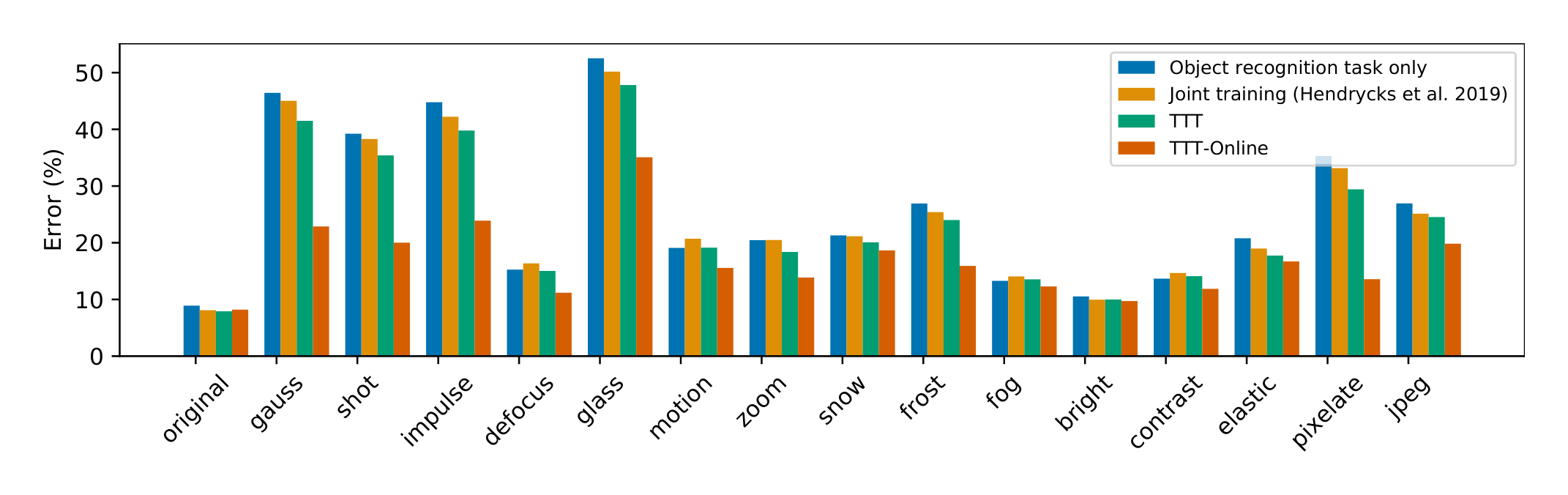
Figure A3. Test error (%) on CIFAR-10-C, level 4. See the results section for details.

: Table A4: Test error (%) on CIFAR-10-C, level 4, ResNet-26.

\begin{tabular}{c|c|c|c|c|c|c|c|c|c|c|c|c|c|c|c|c}
\hline
& orig & gauss & shot & impul & defoc & glass & motn & zoom & snow & frost & fog & brit & contr & elast & pixel & jpeg \\
\hline
B & 8.9 & 46.4 & 39.2 & 44.8 & 15.3 & 52.5 & 19.1 & 20.5 & 21.3 & 26.9 & 13.3 & 10.5 & 13.7 & 20.8 & 35.3 & 26.9 \\
\hline
JT & 8.1 & 45.0 & 38.3 & 42.2 & 16.4 & 50.2 & 20.7 & 20.5 & 21.1 & 25.4 & 14.1 & 10.0 & 14.7 & 19.0 & 33.2 & 25.1 \\
\hline
TTT & 7.9 & 41.5 & 35.4 & 39.8 & 15.0 & 47.8 & 19.1 & 18.4 & 20.1 & 24.0 & 13.5 & 10.0 & 14.1 & 17.7 & 29.4 & 24.5 \\
\hline
TTT-Online & 8.2 & 22.9 & 20.0 & 23.9 & 11.2 & 35.1 & 15.6 & 13.8 & 18.6 & 15.9 & 12.3 & 9.7 & 11.9 & 16.7 & 13.6 & 19.8 \\
\hline
ALP & 16.5 & 21.3 & 20.5 & 24.5 & 20.7 & 25.9 & 23.7 & 21.4 & 24.2 & 23.9 & 42.2 & 17.5 & 53.7 & 22.1 & 19.1 & 18.5 \\
\hline
\end{tabular}

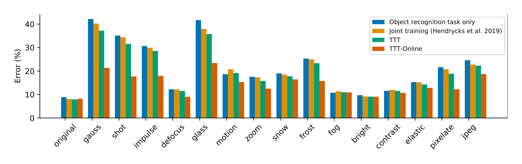
Figure A4. Test error (%) on CIFAR-10-C, level 3. See the results section for details.

: Table A5: Test error (%) on CIFAR-10-C, level 3, ResNet-26.

\begin{tabular}{c|c|c|c|c|c|c|c|c|c|c|c|c|c|c|c|c}
\hline
& orig & gauss & shot & impul & defoc & glass & motn & zoom & snow & frost & fog & brit & contr & elast & pixel & jpeg \\
\hline
B & 8.9 & 42.2 & 35.1 & 30.7 & 12.2 & 41.7 & 18.6 & 17.5 & 19.0 & 25.3 & 10.8 & 9.7 & 11.6 & 15.3 & 21.7 & 24.6 \\
\hline
JT & 8.1 & 40.2 & 34.4 & 29.9 & 12.2 & 37.9 & 20.8 & 17.3 & 18.4 & 25.0 & 11.4 & 9.2 & 12.0 & 15.2 & 20.8 & 22.8 \\
\hline
TTT & 7.9 & 37.2 & 31.6 & 28.6 & 11.5 & 35.8 & 19.1 & 15.8 & 17.8 & 23.3 & 11.0 & 9.1 & 11.6 & 14.3 & 18.9 & 22.3 \\
\hline
TTT-Online & 8.2 & 21.3 & 17.7 & 17.9 & 9.0 & 23.4 & 15.3 & 12.5 & 16.4 & 15.8 & 10.9 & 9.0 & 10.7 & 12.8 & 12.2 & 18.7 \\
\hline
ALP & 16.5 & 20.0 & 19.3 & 20.5 & 19.2 & 21.2 & 24.0 & 20.5 & 20.9 & 24.2 & 30.1 & 16.6 & 39.6 & 20.9 & 17.8 & 18.0 \\
\hline
\end{tabular}

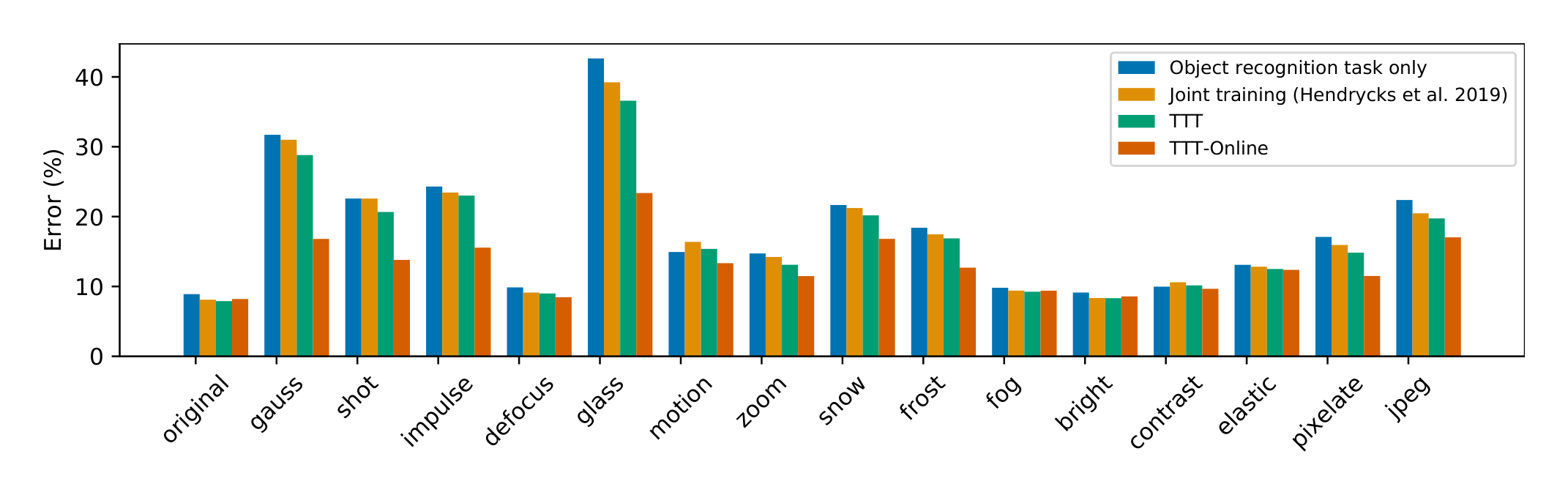
Figure A5. Test error (%) on CIFAR-10-C, level 2. See the results section for details.

: Table A6: Test error (%) on CIFAR-10-C, level 2, ResNet-26.

\begin{tabular}{c|c|c|c|c|c|c|c|c|c|c|c|c|c|c|c|c}
\hline
& orig & gauss & shot & impul & defoc & glass & motn & zoom & snow & frost & fog & brit & contr & elast & pixel & jpeg \\
\hline
B & 8.9 & 31.7 & 22.6 & 24.3 & 9.9 & 42.6 & 14.9 & 14.7 & 21.7 & 18.4 & 9.8 & 9.1 & 10.0 & 13.1 & 17.1 & 22.4 \\
\hline
JT & 8.1 & 31.0 & 22.6 & 23.4 & 9.1 & 39.2 & 16.4 & 14.2 & 21.2 & 17.5 & 9.4 & 8.3 & 10.6 & 12.8 & 15.9 & 20.5 \\
\hline
TTT & 7.9 & 28.8 & 20.7 & 23.0 & 9.0 & 36.6 & 15.4 & 13.1 & 20.2 & 16.9 & 9.2 & 8.3 & 10.2 & 12.5 & 14.8 & 19.7 \\
\hline
TTT-Online & 8.2 & 16.8 & 13.8 & 15.5 & 8.5 & 23.4 & 13.3 & 11.5 & 16.8 & 12.7 & 9.4 & 8.4 & 9.7 & 12.4 & 11.5 & 17.0 \\
\hline
ALP & 16.5 & 18.0 & 17.2 & 19.0 & 17.8 & 20.7 & 21.2 & 19.3 & 19.0 & 20.1 & 22.4 & 16.3 & 29.2 & 20.3 & 17.4 & 17.8 \\
\hline
\end{tabular}

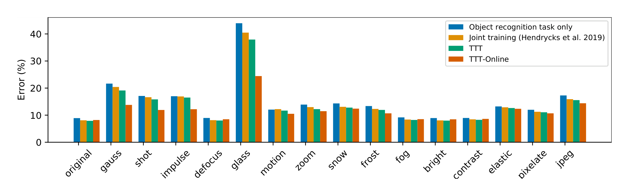
Figure A6. Test error (%) on CIFAR-10-C, level 1. See the results section for details.

: Table A7: Test error (%) on CIFAR-10-C, level 1, ResNet-26.

\begin{tabular}{c|c|c|c|c|c|c|c|c|c|c|c|c|c|c|c|c}
\hline
& orig & gauss & shot & impul & defoc & glass & motn & zoom & snow & frost & fog & brit & contr & elast & pixel & jpeg \\
\hline
B & 8.9 & 21.7 & 17.1 & 17.0 & 9.0 & 44.0 & 12.1 & 13.9 & 14.3 & 13.4 & 9.2 & 8.9 & 9.0 & 13.2 & 12.0 & 17.3 \\
\hline
JT & 8.1 & 20.4 & 16.6 & 16.9 & 8.2 & 40.5 & 12.2 & 13.0 & 13.1 & 12.3 & 8.4 & 8.1 & 8.5 & 12.9 & 11.3 & 15.9 \\
\hline
TTT & 7.9 & 19.1 & 15.8 & 16.5 & 8.0 & 37.9 & 11.7 & 12.2 & 12.8 & 11.9 & 8.2 & 8.0 & 8.3 & 12.6 & 11.1 & 15.5 \\
\hline
TTT-Online & 8.2 & 13.8 & 11.9 & 12.2 & 8.5 & 24.4 & 10.5 & 11.5 & 12.4 & 10.7 & 8.5 & 8.3 & 8.6 & 12.4 & 10.7 & 14.4 \\
\hline
ALP & 17.0 & 16.8 & 17.6 & 16.8 & 20.9 & 18.7 & 19.0 & 17.3 & 17.5 & 17.4 & 16.1 & 18.4 & 20.4 & 17.0 & 17.2 & 17.5 \\
\hline
\end{tabular}

Figure A7. Sample Images from the VID-Robust dataset (Shankar et al., 2019) in the results section adapted to CIFAR-10. Each row shows eight sample images from one class. The seven classes shown are, in order: airplane, bird, car, dog, cat, horse, ship.