Maximum Classifier Discrepancy for Unsupervised Domain Adaptation

Kuniaki SaitoKohei WatanabeYoshitaka UshikuTatsuya Harada

article2017CVPR2,031 citations

Proposes an unsupervised domain adaptation method that aligns feature distributions using task-specific decision boundaries by playing a minimax game on the discrepancy between two distinct classifiers.

Listen

Modern computer vision models require large volumes of labeled training data, which are costly and time-consuming to collect. While models can be trained on readily available labeled data (such as synthetic renderings or web images), they frequently fail when deployed in real-world conditions due to variations in lighting, noise, and viewpoint. Unsupervised domain adaptation seeks to transfer knowledge from a labeled source domain to an unlabeled target domain. However, existing methods primarily focus on matching overall feature distributions without considering decision boundaries between categories, leading to ambiguous, misclassified features near class boundaries.

The article sets out to demonstrate a new unsupervised domain adaptation framework that aligns source and target data by directly utilizing task-specific decision boundaries rather than standard domain discriminators.

The authors designed a minimax training strategy involving a feature generator and two distinct task-specific classifiers. First, both classifiers and the generator learn to classify labeled source samples accurately. Next, the classifiers are trained to maximize their prediction disagreement (discrepancy) on unlabeled target samples, identifying target instances that lie outside the source distribution's boundary. Finally, the feature generator is updated to minimize this discrepancy, forcing target representations into regions where class predictions agree. The method was rigorously evaluated across digit benchmarks (MNIST, SVHN, USPS), traffic sign recognition (SYN SIGNS to GTSRB), large-scale object classification (VisDA, comprising over 280,000 images), and synthetic-to-real urban semantic segmentation (GTA5/Synthia to Cityscapes).

The evaluation produced several key findings: First, the proposed approach consistently outperformed existing distribution-matching methods across all benchmark suites. Second, on the large-scale VisDA synthetic-to-real classification benchmark, the method achieved an overall accuracy of 71.9%, outperforming competitive baselines like DANN (57.4%) and MMD (61.1%), as well as exceeding the source-only baseline across every individual object category. Third, in complex urban semantic segmentation using deep residual networks, the method improved mean intersection-over-union scores from 22.2% to 39.7% on GTA5-to-Cityscapes and from 23.4% to 37.3% on Synthia-to-Cityscapes, visibly producing sharper object boundaries. Fourth, increasing the number of generator update steps per iteration consistently enhanced adaptation performance across tasks.

These findings indicate that incorporating task-specific boundary awareness into domain adaptation avoids ambiguous feature generation and significantly improves transfer performance. For organizations deploying machine vision systems, this approach reduces the risk of deployment failure and substantially cuts data labeling costs by enabling robust deployment from synthetic 3D simulations or public datasets to real-world target environments without requiring target annotations.

Teams implementing visual recognition in domain-shifted environments should adopt discrepancy-based alignment strategies over traditional domain classifiers. When applying the technique to complex domain gaps (such as synthetic-to-real transfers), practitioners should allocate multiple generator update iterations per training batch to balance discriminator-generator trade-offs. Further work should explore automated tuning for generator update frequencies and test the approach under broader operational conditions where class distributions may not fully overlap.

Confidence in these findings is high, as the method is grounded in established statistical learning theory and demonstrated superior performance across diverse visual recognition tasks. However, users should note that the evaluation assumes identical class categories across domains and relied on fixed training hyperparameters without target-domain validation tuning, which may require careful calibration in production pipelines.

  • Paper: Conditional Adversarial Domain Adaptation, Mingsheng Long et al. (2017). It addresses the same challenge of class-boundary ambiguity in adversarial adaptation by conditioning domain discriminators on classifier predictions.
  • Paper: Deep Visual Domain Adaptation: A Survey, Mei Wang et al. (2018). It provides a comprehensive survey and taxonomy of deep visual domain adaptation methods, framing discrepancy and adversarial approaches like the source paper in broader context.
  • Paper: CyCADA: Cycle-Consistent Adversarial Domain Adaptation, Judy Hoffman et al. (2018). It extends unsupervised domain adaptation to joint pixel- and feature-level alignment for complex visual tasks including semantic segmentation.
  • Paper: Moment Matching for Multi-Source Domain Adaptation, Xingchao Peng et al. (2018). It generalizes unsupervised domain adaptation paradigms to the multi-source setting with Moment Matching and the large-scale DomainNet benchmark.
  • Paper: A Survey on Deep Transfer Learning, Chuanqi Tan et al. (2018). It synthesizes mapping-based and adversarial transfer learning frameworks across deep neural network architectures.
  • Paper: A Comprehensive Survey on Transfer Learning, Fuzhen Zhuang et al. (2019). It offers an extensive comparative overview of homogeneous and heterogeneous transfer learning strategies and alignment mechanisms.
Cover for Maximum Classifier Discrepancy for Unsupervised Domain Adaptation

Abstract

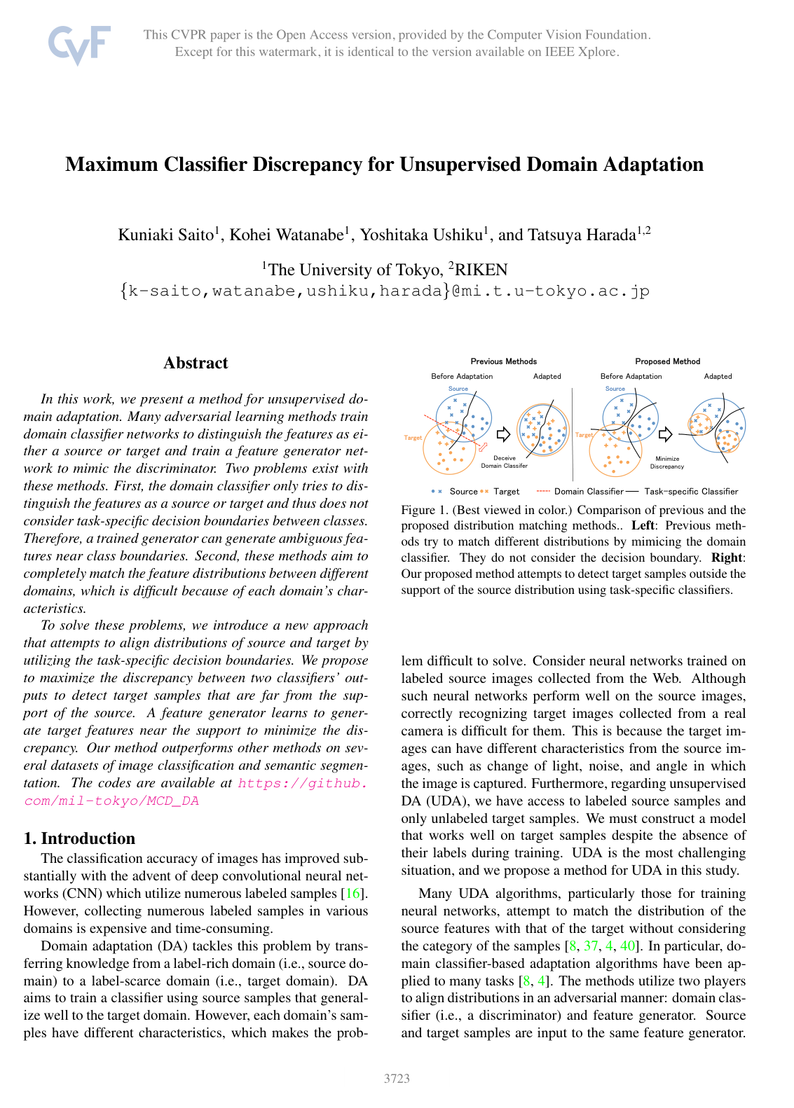
In this work, we present a method for unsupervised domain adaptation. Many adversarial learning methods train domain classifier networks to distinguish the features as either a source or target and train a feature generator network to mimic the discriminator. Two problems exist with these methods. First, the domain classifier only tries to distinguish the features as a source or target and thus does not consider task-specific decision boundaries between classes. Therefore, a trained generator can generate ambiguous features near class boundaries. Second, these methods aim to completely match the feature distributions between different domains, which is difficult because of each domain's characteristics.

To solve these problems, we introduce a new approach that attempts to align distributions of source and target by utilizing the task-specific decision boundaries. We propose to maximize the discrepancy between two classifiers' outputs to detect target samples that are far from the support of the source. A feature generator learns to generate target features near the support to minimize the discrepancy. Our method outperforms other methods on several datasets of image classification and semantic segmentation. The codes are available at \url{this https URL}

Table of Contents

  • 1 Introduction
  • 2 Related Work
  • 3 Method
  • 3.1 Overall Idea
  • 3.2 Discrepancy Loss
  • 3.3 Training Steps
  • 3.4 Theoretical Insight
  • 4 Experiments on Classification
  • 4.1 Experiments on Toy Datasets
  • 4.2 Experiments on Digits Datasets
  • 4.3 Experiments on VisDA Classification Dataset
  • 5 Experiments on Semantic Segmentation
  • 6 Conclusion
  • 7 Acknowledgements
  • References

Knowls

  1. Knowl 1 — Maximum Classifier Discrepancy Framework for Unsupervised Domain Adaptation

    model/method

    The Maximum Classifier Discrepancy (MCD) framework addresses unsupervised domain adaptation (UDA) by aligning source and target feature distributions using task-specific decision boundaries rather than a domain discriminator.

    In standard domain-adversarial approaches, a domain discriminator is trained to distinguish source from target features, and a generator is trained to fool it. Because the discriminator ignores class boundaries, the generator can produce ambiguous features near decision boundaries. MCD replaces the domain discriminator with two task-specific classifiers, F1F_1 and F2F_2, that take feature representations from a shared feature generator GG.

    Given labeled source samples (xs,ys)hicksim(Xs,Ys)(x_s, y_s) hicksim (X_s, Y_s) and unlabeled target samples xthicksimXtx_t hicksim X_t, the classifiers F1F_1 and F2F_2 are trained to classify source samples correctly while maximizing the discrepancy between their predictions on target samples. Target samples residing outside the support of the source distribution fall in regions where the two distinct classifiers disagree. Simultaneously, the generator GG is trained adversarially to minimize this classifier discrepancy, forcing target representations to be generated within the support of the source domain. This ensures that target features are discriminative and align with class-specific decision boundaries without requiring domain labels.

  2. Knowl 2 — Three-Step Adversarial Training Procedure for Maximum Classifier Discrepancy

    algorithm

    The MCD training process alternates across three optimization steps to align feature distributions according to task-specific decision boundaries:

    1. Step A (Source Classification Training): Both the feature generator GG and the two classifiers F1,F2F_1, F_2 are trained to classify labeled source samples correctly by minimizing standard multi-class cross-entropy loss: min⁡G,F1,F2L(Xs,Ys)=−E(xs,ys)∼(Xs,Ys)∑k=1KI[k=ys]log⁡p(y=k∣xs)\min_{G, F_1, F_2} \mathcal{L}(X_s, Y_s) = -\mathbb{E}_{(x_s, y_s) \sim (X_s, Y_s)} \sum_{k=1}^K \mathbb{I}[k = y_s] \log p(y=k \mid x_s)

    2. Step B (Classifier Discrepancy Maximization): Generator GG is fixed. Classifiers F1F_1 and F2F_2 are updated to maximize prediction discrepancy on target samples while retaining source classification accuracy: min⁡F1,F2L(Xs,Ys)−Ladv(Xt)\min_{F_1, F_2} \mathcal{L}(X_s, Y_s) - \mathcal{L}_{adv}(X_t) Retaining the source loss L(Xs,Ys)\mathcal{L}(X_s, Y_s) is essential; omitting it significantly degrades adaptation performance.

    3. Step C (Generator Discrepancy Minimization): Classifiers F1F_1 and F2F_2 are fixed. The generator GG is updated to minimize target prediction discrepancy: min⁡GLadv(Xt)\min_G \mathcal{L}_{adv}(X_t) To balance the adversarial game between the generator and classifiers, Step C is repeated nn times per mini-batch, where n≥1n \ge 1 is a hyperparameter.

    Input: Labeled source dataset Xs,YsX_s, Y_s, unlabeled target dataset XtX_t, generator repeat factor nn, batch size BB, number of iterations TT
    Output: Trained generator GG, trained classifiers F1,F2F_1, F_2
    Initialize generator GG and classifiers F1,F2F_1, F_2 with different initial weights
    for step in 1 to TT:
        Sample source batch (xs(i),ys(i))i=1B⊂(Xs,Ys){(x_s^{(i)}, y_s^{(i)})}_{i=1}^B \subset (X_s, Y_s)
        Sample target batch xt(i)i=1B⊂Xt{x_t^{(i)}}_{i=1}^B \subset X_t
        
        # Step A: Train G, F1, F2 on source data
        Compute source loss L(Xs,Ys)\mathcal{L}(X_s, Y_s)
        Update G,F1,F2G, F_1, F_2 to minimize L(Xs,Ys)\mathcal{L}(X_s, Y_s)
        
        # Step B: Train F1, F2 to maximize target discrepancy
        Compute target adversarial loss Ladv(Xt)=1B∑i=1Bd(p1(y∣xt(i)),p2(y∣xt(i)))\mathcal{L}_{adv}(X_t) = \frac{1}{B} \sum_{i=1}^B d(p_1(y \mid x_t^{(i)}), p_2(y \mid x_t^{(i)}))
        Update F1,F2F_1, F_2 to minimize L(Xs,Ys)−Ladv(Xt)\mathcal{L}(X_s, Y_s) - \mathcal{L}_{adv}(X_t) with GG fixed
        
        # Step C: Train G to minimize target discrepancy
        for iter in 1 to nn:
            Compute target adversarial loss Ladv(Xt)\mathcal{L}_{adv}(X_t)
            Update GG to minimize Ladv(Xt)\mathcal{L}_{adv}(X_t) with F1,F2F_1, F_2 fixed
  3. Knowl 3 — Classifier Discrepancy Loss

    equation

    For a KK-class classification task, let p1(y∣x)p_1(y \mid x) and p2(y∣x)p_2(y \mid x) denote the KK-dimensional class probability vectors output by classifiers F1F_1 and F2F_2 after applying softmax to their respective logit outputs for input xx. The discrepancy d(p1,p2)d(p_1, p_2) between the two classifiers on an input sample is defined as the mean L1L_1-distance between their predicted class probabilities:

    d(p1,p2)=1K∑k=1K∣p1k−p2k∣d(p_1, p_2) = \frac{1}{K} \sum_{k=1}^K |p_{1k} - p_{2k}|

    where p1kp_{1k} and p2kp_{2k} are the predicted probabilities for class k∈{1,…,K}k \in \{1, \dots, K\}.

    The expected adversarial discrepancy loss over the target domain XtX_t is:

    Ladv(Xt)=Ext∼Xt[d(p1(y∣xt),p2(y∣xt))]\mathcal{L}_{adv}(X_t) = \mathbb{E}_{x_t \sim X_t} \left[ d(p_1(y \mid x_t), p_2(y \mid x_t)) \right]

    The use of L1L_1-distance is theoretically grounded in the definition of the HΔH\mathcal{H}\Delta\mathcal{H}-distance. L2L_2-distance does not perform effectively for this objective.

  4. Knowl 4 — Theoretical Connection between Maximum Classifier Discrepancy and the Target Error Bound

    theoretical result

    According to domain adaptation theory (Ben-David et al., 2010), the target error RT(h)R_T(h) of a hypothesis hh from hypothesis class H\mathcal{H} is upper-bounded by:

    ∀h∈H,RT(h)≤RS(h)+12dHΔH(S,T)+λ≤RS(h)+12dH(S,T)+λ\forall h \in \mathcal{H}, \quad R_T(h) \le R_S(h) + \frac{1}{2} d_{\mathcal{H}\Delta\mathcal{H}}(S, T) + \lambda \le R_S(h) + \frac{1}{2} d_{\mathcal{H}}(S, T) + \lambda

    where RS(h)R_S(h) is the expected source error, λ=min⁡h′∈H[RS(h′)+RT(h′)]\lambda = \min_{h' \in \mathcal{H}} [R_S(h') + R_T(h')] is the error of the ideal joint hypothesis, and the HΔH\mathcal{H}\Delta\mathcal{H}-distance between source domain SS and target domain TT is defined as:

    dHΔH(S,T)=2sup⁡(h,h′)∈H2∣Ex∼SI[h(x)≠h′(x)]−Ex∼TI[h(x)≠h′(x)]∣d_{\mathcal{H}\Delta\mathcal{H}}(S, T) = 2 \sup_{(h, h') \in \mathcal{H}^2} \left| \mathbb{E}_{x \sim S} \mathbb{I}[h(x) \neq h'(x)] - \mathbb{E}_{x \sim T} \mathbb{I}[h(x) \neq h'(x)] \right|

    When hypotheses hh and h′h' are trained to correctly classify source samples, their source disagreement Ex∼SI[h(x)≠h′(x)]\mathbb{E}_{x \sim S} \mathbb{I}[h(x) \neq h'(x)] is approximately zero. Consequently, the HΔH\mathcal{H}\Delta\mathcal{H}-distance reduces to the supremum of classifier disagreement on target samples:

    dHΔH(S,T)≈2sup⁡(h,h′)∈H2Ex∼TI[h(x)≠h′(x)]d_{\mathcal{H}\Delta\mathcal{H}}(S, T) \approx 2 \sup_{(h, h') \in \mathcal{H}^2} \mathbb{E}_{x \sim T} \mathbb{I}[h(x) \neq h'(x)]

    Decomposing hypotheses into a shared feature extractor GG and classifiers F1,F2F_1, F_2 (such that h=F1∘Gh = F_1 \circ G and h′=F2∘Gh' = F_2 \circ G), minimizing the target error bound corresponds to the minimax formulation:

    min⁡Gmax⁡F1,F2Ex∼TI[F1(G(x))≠F2(G(x))]\min_G \max_{F_1, F_2} \mathbb{E}_{x \sim T} \mathbb{I}[F_1(G(x)) \neq F_2(G(x))]

    This minimax formulation provides the theoretical foundation for MCD's adversarial optimization.

  5. Knowl 5 — Benchmark Results on Visual Digit and Traffic Sign Adaptation Datasets

    data/table

    The MCD method was evaluated on standard unsupervised visual adaptation benchmarks: SVHN →\to MNIST, Synthetic Traffic Signs (SYN SIGNS) →\to GTSRB (43 classes), MNIST →\to USPS, and USPS →\to MNIST. Networks were optimized using Adam with learning rate 2.0×10−42.0 \times 10^{-4} and batch size 128 without using target validation samples for hyperparameter tuning. Results report mean ±\pm standard deviation over 5 runs using classifier F1F_1.

    Method SVHN →\to MNIST SYN SIGNS →\to GTSRB MNIST →\to USPS MNIST* →\to USPS* USPS →\to MNIST
    Source Only 67.1 85.1 76.7 79.4 63.4
    MMD 71.1 91.1 – 81.1 –
    DANN 71.1 88.7 77.1 ±\pm 1.8 85.1 73.0 ±\pm 0.2
    DSN 82.7 93.1 91.3 – –
    ADDA 76.0 ±\pm 1.8 – 89.4 ±\pm 0.2 – 90.1 ±\pm 0.8
    CoGAN – – 91.2 ±\pm 0.8 – 89.1 ±\pm 0.8
    PixelDA – – – 95.9 –
    MCD (n=2n=2) 94.2 ±\pm 2.6 93.5 ±\pm 0.4 92.1 ±\pm 0.8 93.1 ±\pm 1.9 90.0 ±\pm 1.4
    MCD (n=3n=3) 95.9 ±\pm 0.5 94.0 ±\pm 0.4 93.8 ±\pm 0.8 95.6 ±\pm 0.9 91.8 ±\pm 0.9
    MCD (n=4n=4) 96.2 ±\pm 0.4 94.4 ±\pm 0.3 94.2 ±\pm 0.7 96.5 ±\pm 0.3 94.1 ±\pm 0.3

    Note: MNIST* and USPS* denote using all available training samples.

    MCD outperforms previous distribution-matching methods across all benchmark scenarios. Increasing the generator update frequency nn from 2 to 4 consistently improves target accuracy.

  6. Knowl 6 — Synthetic-to-Real Object Classification Accuracy on the VisDA Dataset

    data/table

    MCD was evaluated on the VisDA 2017 cross-domain object classification challenge, which transfers from 152,397 synthetic 3D CAD rendered images (source domain) to 55,388 real images from MSCOCO (target domain) across 12 object categories. A ResNet-101 backbone pre-trained on ImageNet was used as generator GG, with three-layer fully connected networks as classifiers F1,F2F_1, F_2. Training used SGD with learning rate 1.0×10−31.0 \times 10^{-3} and batch size 32 for 10 epochs.

    Method plane bcycl bus car horse knife mcycl person plant sktbrd train truck mean
    Source Only 55.1 53.3 61.9 59.1 80.6 17.9 79.7 31.2 81.0 26.5 73.5 8.5 52.4
    MMD 87.1 63.0 76.5 42.0 90.3 42.9 85.9 53.1 49.7 36.3 85.8 20.7 61.1
    DANN 81.9 77.7 82.8 44.3 81.2 29.5 65.1 28.6 51.9 54.6 82.8 7.8 57.4
    MCD (n=2n=2) 81.1 55.3 83.6 65.7 87.6 72.7 83.1 73.9 85.3 47.7 73.2 27.1 69.7
    MCD (n=3n=3) 90.3 49.3 82.1 62.9 91.8 69.4 83.8 72.8 79.8 53.3 81.5 29.7 70.6
    MCD (n=4n=4) 87.0 60.9 83.7 64.0 88.9 79.6 84.7 76.9 88.6 40.3 83.0 25.8 71.9

    MCD achieves a mean accuracy of 71.9% (n=4n=4), substantially outperforming MMD (61.1%) and DANN (57.4%). Notably, while MMD and DANN experience negative transfer on classes like car (42.0% and 44.3% vs. 59.1% Source Only) and plant (49.7% and 51.9% vs. 81.0% Source Only), MCD outperforms the Source Only baseline across every individual category.

  7. Knowl 7 — Synthetic-to-Real Semantic Segmentation Results on GTA5 and Synthia to Cityscapes

    data/table

    MCD was evaluated on semantic segmentation domain adaptation using synthetic source datasets (GTA5 and Synthia) and the real Cityscapes dataset (target domain, evaluated on the validation set). Architectures evaluated include VGG-16 based FCN-8s and DRN-D-105. Models were trained using Momentum SGD (learning rate 1.0×10−31.0 \times 10^{-3}, momentum 0.9, batch size 1, input resized to 1024×5121024 \times 512) for 50,000 iterations.

    Network Method mIoU (GTA5 →\to Cityscapes) mIoU (Synthia →\to Cityscapes)
    VGG-16 Source Only 24.9 22.0
    VGG-16 FCN Wild 27.1 20.2
    VGG-16 CDA 23.1 29.0
    VGG-16 MCD (n=2n=2) 28.0 –
    VGG-16 MCD (n=3n=3) 27.3 –
    VGG-16 MCD (n=4n=4) 28.8 –
    DRN-105 Source Only 22.2 23.4
    DRN-105 DANN 32.8 32.5
    DRN-105 MCD (n=2n=2) 39.7 36.3
    DRN-105 MCD (n=3n=3) 38.9 37.3
    DRN-105 MCD (n=4n=4) 38.1 37.2

    For GTA5 o o Cityscapes with DRN-105, MCD achieves 39.7% mIoU compared to 32.8% for DANN and 22.2% for Source Only. On Synthia o o Cityscapes with DRN-105, MCD achieves 37.3% mIoU compared to 32.5% for DANN and 23.4% for Source Only.

  8. Knowl 8 — Decision Boundary Dynamics on Intertwining Moons Toy Dataset

    empirical result

    The operational mechanism of MCD was demonstrated on a 2D synthetic problem using intertwining moons (300 source and 300 target samples per class, tested on 1,000 target samples), where the target distribution was generated by rotating the two source moon distributions:

    1. Source Only Model: When two classifiers are trained only on labeled source samples without adaptation, their learned decision boundaries align closely with each other on the source distribution but fail to account for the rotated target distribution, misclassifying target points.

    2. Discrepancy Maximization without Generator Step (No Step C): When classifiers are trained to maximize discrepancy on target samples while classifying source samples correctly (skipping Step C), the two classifiers diverge widely across target samples that lie outside the source support, clearly demarcating the discrepancy region.

    3. Full MCD Model: With Step C included, the generator learns to produce target representations that minimize classifier disagreement, pulling target representations into the support of the source classes. Consequently, the two decision boundaries adapt to separate the target distribution accurately, achieving correct classification across the vast majority of target points.

Coverage note — None was omitted; all core contributions, theoretical justifications, algorithmic steps, and empirical results across visual classification and semantic segmentation benchmarks are covered.

References

  1. 1.S. Ben-David, J. Blitzer, K. Crammer, A. Kulesza, F. Pereira, and J. W. Vaughan. A theory of learning from different domains. Machine learning, 79(1-2):151–175, 2010.
  2. 2.S. Ben-David, J. Blitzer, K. Crammer, F. Pereira, et al. Analysis of representations for domain adaptation. In NIPS, 2007.
  3. 3.K. Bousmalis, N. Silberman, D. Dohan, D. Erhan, and D. Krishnan. Unsupervised pixel-level domain adaptation with generative adversarial networks. In CVPR, 2017.
  4. 4.K. Bousmalis, G. Trigeorgis, N. Silberman, D. Krishnan, and D. Erhan. Domain separation networks. In NIPS, 2016.
  5. 5.M. Cordts, M. Omran, S. Ramos, T. Rehfeld, M. Enzweiler, R. Benenson, U. Franke, S. Roth, and B. Schiele. The cityscapes dataset for semantic urban scene understanding. In CVPR, 2016.
  6. 6.J. Deng, W. Dong, R. Socher, L.-J. Li, K. Li, and L. Fei-Fei. Imagenet: A large-scale hierarchical image database. In CVPR, 2009.
  7. 7.Y. Ganin and V. Lempitsky. Unsupervised domain adaptation by backpropagation. In ICML, 2014.
  8. 8.Y. Ganin, E. Ustinova, H. Ajakan, P. Germain, H. Larochelle, F. Laviolette, M. Marchand, and V. Lempitsky. Domain-adversarial training of neural networks. JMLR, 17(59):1–35, 2016.
  9. 9.M. Ghifary, W. B. Kleijn, M. Zhang, D. Balduzzi, and W. Li. Deep reconstruction-classification networks for unsupervised domain adaptation. In ECCV, 2016.
  10. 10.I. Goodfellow, J. Pouget-Abadie, M. Mirza, B. Xu, D. Warde-Farley, S. Ozair, A. Courville, and Y. Bengio. Generative adversarial nets. In Z. Ghahramani, M. Welling, C. Cortes, N. D. Lawrence, and K. Q. Weinberger, editors, NIPS, 2014.
  11. 11.P. Haeusser, T. Frerix, A. Mordvintsev, and D. Cremers. Associative domain adaptation. In ICCV, 2017.
  12. 12.K. He, X. Zhang, S. Ren, and J. Sun. Deep residual learning for image recognition. In CVPR, 2016.
  13. 13.J. Hoffman, D. Wang, F. Yu, and T. Darrell. Fcns in the wild: Pixel-level adversarial and constraint-based adaptation. arXiv:1612.02649, 2016.
  14. 14.J. J. Hull. A database for handwritten text recognition research. PAMI, 16(5):550–554, 1994.
  15. 15.D. Kingma and J. Ba. Adam: A method for stochastic optimization. arXiv:1412.6980, 2014.
  16. 16.A. Krizhevsky, I. Sutskever, and G. E. Hinton. Imagenet classification with deep convolutional neural networks. In NIPS, 2012.
  17. 17.Y. LeCun, L. Bottou, Y. Bengio, and P. Haffner. Gradient-based learning applied to document recognition. Proceedings of the IEEE, 86(11):2278–2324, 1998.
  18. 18.T.-Y. Lin, M. Maire, S. Belongie, J. Hays, P. Perona, D. Ramanan, P. Dollár, and C. L. Zitnick. Microsoft coco: Common objects in context. In ECCV, 2014.
  19. 19.M.-Y. Liu and O. Tuzel. Coupled generative adversarial networks. In NIPS, 2016.
  20. 20.J. Long, E. Shelhamer, and T. Darrell. Fully convolutional networks for semantic segmentation. In CVPR, 2015.
  21. 21.M. Long, Y. Cao, J. Wang, and M. I. Jordan. Learning transferable features with deep adaptation networks. In ICML, 2015.
  22. 22.M. Long, H. Zhu, J. Wang, and M. I. Jordan. Unsupervised domain adaptation with residual transfer networks. In NIPS, 2016.
  23. 23.P. Luo, F. Zhuang, H. Xiong, Y. Xiong, and Q. He. Transfer learning from multiple source domains via consensus regularization. In CIKM, 2008.
  24. 24.L. v. d. Maaten and G. Hinton. Visualizing data using t-sne. JMLR, 9(11):2579–2605, 2008.
  25. 25.B. Moiseev, A. Konev, A. Chigorin, and A. Konushin. Evaluation of traffic sign recognition methods trained on synthetically generated data. In ACIVS, 2013.
  26. 26.Y. Netzer, T. Wang, A. Coates, A. Bissacco, B. Wu, and A. Y. Ng. Reading digits in natural images with unsupervised feature learning. In NIPS workshop on deep learning and unsupervised feature learning, 2011.
  27. 27.F. Pedregosa, G. Varoquaux, A. Gramfort, V. Michel, B. Thirion, O. Grisel, M. Blondel, P. Prettenhofer, R. Weiss, V. Dubourg, et al. Scikit-learn: Machine learning in python. JMLR, 12(10):2825–2830, 2011.
  28. 28.X. Peng, B. Usman, N. Kaushik, J. Hoffman, D. Wang, and K. Saenko. Visda: The visual domain adaptation challenge. arXiv:1710.06924, 2017.
  29. 29.S. Purushotham, W. Carvalho, T. Nilanon, and Y. Liu. Variational recurrent adversarial deep domain adaptation. In ICLR, 2017.
  30. 30.S. R. Richter, V. Vineet, S. Roth, and V. Koltun. Playing for data: Ground truth from computer games. In ECCV, 2016.
  31. 31.G. Ros, L. Sellart, J. Materzynska, D. Vazquez, and A. M. Lopez. The synthia dataset: A large collection of synthetic images for semantic segmentation of urban scenes. In CVPR, 2016.
  32. 32.K. Saito, Y. Ushiku, and T. Harada. Asymmetric tri-training for unsupervised domain adaptation. In ICML, 2017.
  33. 33.O. Sener, H. O. Song, A. Saxena, and S. Savarese. Learning transferrable representations for unsupervised domain adaptation. In NIPS, 2016.
  34. 34.K. Simonyan and A. Zisserman. Very deep convolutional networks for large-scale image recognition. arXiv:1409.1556, 2014.
  35. 35.J. Stallkamp, M. Schlipsing, J. Salmen, and C. Igel. The german traffic sign recognition benchmark: a multi-class classification competition. In IJCNN, 2011.
  36. 36.B. Sun, J. Feng, and K. Saenko. Return of frustratingly easy domain adaptation. In AAAI, 2016.
  37. 37.B. Sun and K. Saenko. Deep coral: Correlation alignment for deep domain adaptation. In ECCV Workshops, 2016.
  38. 38.Y. Taigman, A. Polyak, and L. Wolf. Unsupervised cross-domain image generation. In ICLR, 2017.
  39. 39.E. Tzeng, J. Hoffman, K. Saenko, and T. Darrell. Adversarial discriminative domain adaptation. In CVPR, 2017.
  40. 40.E. Tzeng, J. Hoffman, N. Zhang, K. Saenko, and T. Darrell. Deep domain confusion: Maximizing for domain invariance. arXiv:1412.3474, 2014.
  41. 41.F. Yu, V. Koltun, and T. Funkhouser. Dilated residual networks. In CVPR, 2017.
  42. 42.Y. Zhang, P. David, and B. Gong. Curriculum domain adaptation for semantic segmentation of urban scenes. In ICCV, 2017.

Citation

MLA
Saito, K., et al. “Maximum Classifier Discrepancy for Unsupervised Domain Adaptation”. arXiv, 2017, http://arxiv.org/abs/1712.02560v4.
APA
Saito, K., Watanabe, K., Ushiku, Y., & Harada, T. (2017). Maximum Classifier Discrepancy for Unsupervised Domain Adaptation. arXiv. http://arxiv.org/abs/1712.02560v4
Chicago
Saito, K., K. Watanabe, Y. Ushiku, and T. Harada. 2017. “Maximum Classifier Discrepancy for Unsupervised Domain Adaptation”. arXiv. http://arxiv.org/abs/1712.02560v4.
Harvard
Saito, K. et al. (2017) “Maximum Classifier Discrepancy for Unsupervised Domain Adaptation”, arXiv [Preprint]. Available at: http://arxiv.org/abs/1712.02560v4.
Vancouver
1. Saito K, Watanabe K, Ushiku Y, Harada T (2017) Maximum Classifier Discrepancy for Unsupervised Domain Adaptation. arXiv

BibTeX

@article{saito2017maximum,
  title = {Maximum Classifier Discrepancy for Unsupervised Domain Adaptation},
  author = {Saito, Kuniaki and Watanabe, Kohei and Ushiku, Yoshitaka and Harada, Tatsuya},
  year = {2017},
  journal = {arXiv},
  url = {http://arxiv.org/abs/1712.02560v4},
  eprint = {1712.02560}
}
Metadata:arXiv

Source Code

This paper has an official code repository available. Click below to access the source code.

View Repository

Access the Paper

This paper is available from its original source. Click below to access the PDF.

Open PDF

License: IEEE