Domain-Adversarial Training of Neural Networks

Yaroslav Ganin [email protected]

Evgeniya Ustinova [email protected]

Skolkovo Institute of Science and Technology (Skoltech)

Skolkovo, Moscow Region, Russia

Hana Ajakan [email protected]

Pascal Germain [email protected]

Département d'informatique et de génie logiciel,

Université Laval

Québec, Canada,

G1V 0A6

Hugo Larochelle [email protected]

Département d'informatique,

Université de Sherbrooke

Québec, Canada,

J1K 2R1

François Laviolette [email protected]

Mario Marchand [email protected]

Département d'informatique et de génie logiciel,

Université Laval

Québec, Canada,

G1V 0A6

Victor Lempitsky [email protected]

Skolkovo Institute of Science and Technology (Skoltech)

Skolkovo, Moscow Region, Russia

Editors: Urun Dogan, Marius Kloft, Francesco Orabona, and Tatiana Tommasi

Abstract

We introduce a new representation learning approach for domain adaptation, in which data at training and test time come from similar but different distributions. Our approach is directly inspired by the theory on domain adaptation suggesting that, for effective domain transfer to be achieved, predictions must be made based on features that cannot discriminate between the training (source) and test (target) domains.

The approach implements this idea in the context of neural network architectures that are trained on labeled data from the source domain and unlabeled data from the target domain (no labeled target-domain data is necessary). As the training progresses, the approach promotes the emergence of features that are (i) discriminative for the main learning task on the source domain and (ii) indiscriminate with respect to the shift between the domains. We show that this adaptation behaviour can be achieved in almost any feed-forward model by augmenting it with few standard layers and a new gradient reversal layer. The resulting augmented architecture can be trained using standard backpropagation and stochastic gradient descent, and can thus be implemented with little effort using any of the deep learning packages.

We demonstrate the success of our approach for two distinct classification problems (document sentiment analysis and image classification), where state-of-the-art domain adaptation performance on standard benchmarks is achieved. We also validate the approach for descriptor learning task in the context of person re-identification application.

domain adaptation, neural network, representation learning, deep learning, synthetic data, image classification, sentiment analysis, person re-identification

1. Introduction

The cost of generating labeled data for a new machine learning task is often an obstacle for applying machine learning methods. In particular, this is a limiting factor for the further progress of deep neural network architectures, that have already brought impressive advances to the state-of-the-art across a wide variety of machine-learning tasks and applications.

For problems lacking labeled data, it may be still possible to obtain training sets that are big enough for training large-scale deep models, but that suffer from the shift in data distribution from the actual data encountered at "test time". One important example is training an image classifier on synthetic or semi-synthetic images, which may come in abundance and be fully labeled, but which inevitably have a distribution that is different from real images ([1,2,3,4]). Another example is in the context of sentiment analysis in written reviews, where one might have labeled data for reviews of one type of product (e.g./, movies), while having the need to classify reviews of other products (e.g./, books).

Learning a discriminative classifier or other predictor in the presence of a shift between training and test distributions is known as domain adaptation (DA).

The proposed approaches build mappings between the source (training-time) and the target (test-time) domains, so that the classifier learned for the source domain can also be applied to the target domain, when composed with the learned mapping between domains. The appeal of the domain adaptation approaches is the ability to learn a mapping between domains in the situation when the target domain data are either fully unlabeled (unsupervised domain annotation) or have few labeled samples (semi-supervised domain adaptation). Below, we focus on the harder unsupervised case, although the proposed approach (domain-adversarial learning) can be generalized to the semi-supervised case rather straightforwardly.

Unlike many previous papers on domain adaptation that worked with fixed feature representations, we focus on combining domain adaptation and deep feature learning within one training process. Our goal is to embed domain adaptation into the process of learning representation, so that the final classification decisions are made based on features that are both discriminative and invariant to the change of domains, i.e./, have the same or very similar distributions in the source and the target domains. In this way, the obtained feed-forward network can be applicable to the target domain without being hindered by the shift between the two domains. Our approach is motivated by the theory on domain adaptation ([5,6]), that suggests that a good representation for cross-domain transfer is one for which an algorithm cannot learn to identify the domain of origin of the input observation.

We thus focus on learning features that combine (i) discriminativeness and (ii) domain-invariance. This is achieved by jointly optimizing the underlying features as well as two discriminative classifiers operating on these features: (i) the label predictor that predicts class labels and is used both during training and at test time and (ii) the domain classifier that discriminates between the source and the target domains during training. While the parameters of the classifiers are optimized in order to minimize their error on the training set, the parameters of the underlying deep feature mapping are optimized in order to minimize the loss of the label classifier and to maximize the loss of the domain classifier. The latter update thus works adversarially to the domain classifier, and it encourages domain-invariant features to emerge in the course of the optimization.

Crucially, we show that all three training processes can be embedded into an appropriately composed deep feed-forward network, called domain-adversarial neural network (DANN) (illustrated by Figure 10) that uses standard layers and loss functions, and can be trained using standard backpropagation algorithms based on stochastic gradient descent or its modifications (e.g./, SGD with momentum). The approach is generic as a DANN version can be created for almost any existing feed-forward architecture that is trainable by backpropagation. In practice, the only non-standard component of the proposed architecture is a rather trivial gradient reversal layer that leaves the input unchanged during forward propagation and reverses the gradient by multiplying it by a negative scalar during the backpropagation.

We provide an experimental evaluation of the proposed domain-adversarial learning idea over a range of deep architectures and applications. We first consider the simplest DANN architecture where the three parts (label predictor, domain classifier and feature extractor) are linear, and demonstrate the success of domain-adversarial learning for such architecture. The evaluation is performed for synthetic data as well as for the sentiment analysis problem in natural language processing, where DANN improves the state-of-the-art marginalized Stacked Autoencoders (mSDA) of [7] on the common Amazon reviews benchmark.

We further evaluate the approach extensively for an image classification task, and present results on traditional deep learning image data sets---such as MNIST ([8]) and SVHN ([9])---as well as on

\text{O{\scriptsize FFICE}}

benchmarks ([10]), where domain-adversarial learning allows obtaining a deep architecture that considerably improves over previous state-of-the-art accuracy.

Finally, we evaluate domain-adversarial descriptor learning in the context of person re-identification application ([11]), where the task is to obtain good pedestrian image descriptors that are suitable for retrieval and verification. We apply domain-adversarial learning, as we consider a descriptor predictor trained with a Siamese-like loss instead of the label predictor trained with a classification loss. In a series of experiments, we demonstrate that domain-adversarial learning can improve cross-data-set re-identification considerably.

2. Related work

The general approach of achieving domain adaptation

explored under many facets. Over the years, a large part of the literature has focused mainly on linear hypothesis (see for instance [12,13,14,15,16]). More recently, non-linear representations have become increasingly studied, including neural network representations ([17,18]) and most notably the state-of-the-art mSDA ([7]). That literature has mostly focused on exploiting the principle of robust representations, based on the denoising autoencoder paradigm ([19]).

Concurrently, multiple methods of matching the feature distributions in the source and the target domains have been proposed for unsupervised domain adaptation. Some approaches perform this by reweighing or selecting samples from the source domain ([20,21,22]), while others seek an explicit feature space transformation that would map source distribution into the target one ([23,24,15]). An important aspect of the distribution matching approach is the way the (dis)similarity between distributions is measured. Here, one popular choice is matching the distribution means in the kernel-reproducing Hilbert space ([20,21]), whereas [25] and [26] map the principal axes associated with each of the distributions.

Our approach also attempts to match feature space distributions, however this is accomplished by modifying the feature representation itself rather than by reweighing or geometric transformation. Also, our method uses a rather different way to measure the disparity between distributions based on their separability by a deep discriminatively-trained classifier. Note also that several approaches perform transition from the source to the target domain ([24,25]) by changing gradually the training distribution. Among these methods, [27] does this in a "deep" way by the layerwise training of a sequence of deep autoencoders, while gradually replacing source-domain samples with target-domain samples. This improves over a similar approach of [17] that simply trains a single deep autoencoder for both domains. In both approaches, the actual classifier/predictor is learned in a separate step using the feature representation learned by autoencoder(s). In contrast to [17,27], our approach performs feature learning, domain adaptation and classifier learning jointly, in a unified architecture, and using a single learning algorithm (backpropagation). We therefore argue that our approach is simpler (both conceptually and in terms of its implementation). Our method also achieves considerably better results on the popular

\text{O{\scriptsize FFICE}}

benchmark.

While the above approaches perform unsupervised domain adaptation, there are approaches that perform supervised domain adaptation by exploiting labeled data from the target domain. In the context of deep feed-forward architectures, such data can be used to "fine-tune" the network trained on the source domain ([28,29,30]). Our approach does not require labeled target-domain data. At the same time, it can easily incorporate such data when they are available.

An idea related to ours is described in [31]. While their goal is quite different (building generative deep networks that can synthesize samples), the way they measure and minimize the discrepancy between the distribution of the training data and the distribution of the synthesized data is very similar to the way our architecture measures and minimizes the discrepancy between feature distributions for the two domains. Moreover, the authors mention the problem of saturating sigmoids which may arise at the early stages of training due to the significant dissimilarity of the domains. The technique they use to circumvent this issue (the "adversarial" part of the gradient is replaced by a gradient computed with respect to a suitable cost) is directly applicable to our method.

Also, recent and concurrent reports by [32,33] focus on domain adaptation in feed-forward networks. Their set of techniques measures and minimizes the distance between the data distribution means across domains (potentially, after embedding distributions into RKHS). Their approach is thus different from our idea of matching distributions by making them indistinguishable for a discriminative classifier. Below, we compare our approach to [32,33] on the Office benchmark. Another approach to deep domain adaptation, which is arguably more different from ours, has been developed in parallel by [34].

From a theoretical standpoint, our approach is directly derived from the seminal theoretical works of [5,6]. Indeed, DANN directly optimizes the notion of

{\mathcal{H}}

-divergence. We do note the work of [35], in which HMM representations are learned for word tagging using a posterior regularizer that is also inspired by [6]'s work. In addition to the tasks being different---[35] focus on word tagging problems---, we would argue that DANN learning objective more closely optimizes the

{\mathcal{H}}

-divergence, with [35] relying on cruder approximations for efficiency reasons.

A part of this paper has been published as a conference paper ([36]). This version extends [36] very considerably by incorporating the report [37] (presented as part of the Second Workshop on Transfer and Multi-Task Learning), which brings in new terminology, in-depth theoretical analysis and justification of the approach, extensive experiments with the shallow DANN case on synthetic data as well as on a natural language processing task (sentiment analysis). Furthermore, in this version we go beyond classification and evaluate domain-adversarial learning for descriptor learning setting within the person re-identification application.

3. Domain Adaptation

We consider classification tasks where

X

is the input space and

Y=\{0, 1, \ldots, L{-}1\}

is the set of

L

possible labels. Moreover, we have two different distributions over

X\!\times\! Y

, called the source domain

D_S

and the target domain

D_T

. An unsupervised domain adaptation learning algorithm is then provided with a labeled source sample

S

drawn i.i.d. from

D_S

, and an unlabeled target sample

T

drawn i.i.d. from

{{\mathcal{D}}_\text{T}^{_ X}}

, where

{{\mathcal{D}}_\text{T}^{_ X}}

is the marginal distribution of

D_T

over

X

with

N=n+n'

being the total number of samples.

The goal of the learning algorithm is to build a classifier

\eta: X\to Y

with a low target risk

while having no information about the labels of

D_T

3.1 Domain Divergence

To tackle the challenging domain adaptation task, many approaches bound the target error by the sum of the source error and a notion of distance between the source and the target distributions. These methods are intuitively justified by a simple assumption: the source risk is expected to be a good indicator of the target risk when both distributions are similar. Several notions of distance have been proposed for domain adaptation ([5,6,38,39,14]). In this paper, we focus on the

{\mathcal{H}}

-divergence used by [5,6], and based on the earlier work of [40]. Note that we assume in definition 1 below that the hypothesis class

{\mathcal{H}}

is a (discrete or continuous) set of binary classifiers

\eta: X\to\{0, 1\}

.\footnote{As mentioned by [5], the same analysis holds for multiclass setting. However, to obtain the same results when

|Y|>2

, one should assume that

{\mathcal{H}}

is a symmetrical hypothesis class. That is, for all

h\in {\mathcal{H}}

and any permutation of labels

c:Y\to Y

, we have

c(h)\in {\mathcal{H}}

. Note that this is the case for most commonly used neural network architectures.}

Theorem (Definition 1: [5,6,40]). Given two domain distributions

{{\mathcal{D}}_\text{S}^{_ X}}

and

{{\mathcal{D}}_\text{T}^{_ X}}

over

X

, and a hypothesis class

{\mathcal{H}}

, the *

{\mathcal{H}}

-divergence* between

{{\mathcal{D}}_\text{S}^{_ X}}

and

{{\mathcal{D}}_\text{T}^{_ X}}

\begin{align*} d_ {\mathcal{H}}({{\mathcal{D}}_\text{S}^{_ X}}, {{\mathcal{D}}_\text{T}^{_ X}}) & = & 2 \, \sup_{\eta\in {\mathcal{H}}} \, \bigg|\, \Pr_{{\mathbf x} \sim {{\mathcal{D}}_\text{S}^{_ X}}} \big[\eta({\mathbf x}) = 1\big] - \Pr_{{\mathbf x} \sim {{\mathcal{D}}_\text{T}^{_ X}}} \big[\eta({\mathbf x}) = 1\big]\, \bigg|\, . \end{align*}

💭 Click to ask about this equation

That is, the

{\mathcal{H}}

-divergence relies on the capacity of the hypothesis class

{\mathcal{H}}

to distinguish between examples generated by

{{\mathcal{D}}_\text{S}^{_ X}}

from examples generated by

{{\mathcal{D}}_\text{T}^{_ X}}

. [5,6] proved that, for a symmetric hypothesis class

{\mathcal{H}}

, one can compute the empirical ${\mathcal{H}}$ -divergence between two samples

S\sim({{\mathcal{D}}_\text{S}^{_ X}})^n

and

T\sim({{\mathcal{D}}_\text{T}^{_ X}})^{n'}

by computing

\begin{align} \hat{d}_ {\mathcal{H}}(S, T) & = & 2\, \Bigg(1 - \min_{\eta\in {\mathcal{H}}} \bigg[\frac{1}{n} \sum_{i=1}^n I[\eta({\mathbf x}_i)\!=\!0] + \frac{1}{n'} \sum_{i=n+1}^{N} I[\eta({\mathbf x}_i)\!=\!1] \bigg] \Bigg)\, , \end{align}\tag{1}

💭 Click to ask about this equation

where

I[a]

is the indicator function which is

1

if predicate

a

is true, and

0

otherwise.

3.2 Proxy Distance

[5] suggested that, even if it is generally hard to compute

\hat{d}_ {\mathcal{H}}(S, T)

exactly (e.g./, when

{\mathcal{H}}

is the space of linear classifiers on

X

), we can easily approximate it by running a learning algorithm on the problem of discriminating between source and target examples. To do so, we construct a new data set

where the examples of the source sample are labeled

0

and the examples of the target sample are labeled

1

. Then, the risk of the classifier trained on the new data set

U

approximates the "

\min

" part of Equation 1. Given a generalization error

\epsilon

on the problem of discriminating between source and target examples, the

{\mathcal{H}}

-divergence is then approximated by

In [5], the value

\hat{d}_ {\mathcal{A}}

is called the Proxy ${\mathcal{A}}$ -distance (PAD). The *

{\mathcal{A}}

-distance* being defined as

d_ {\mathcal{A}}({{\mathcal{D}}_\text{S}^{_ X}}, {{\mathcal{D}}_\text{T}^{_ X}}) = 2 \, \sup_{A\in {\mathcal{A}}} \, \big|\, \Pr_{{{\mathcal{D}}_\text{S}^{_ X}}} (A) - \Pr_{{{\mathcal{D}}_\text{T}^{_ X}}} (A)\, \big|

, where

{\mathcal{A}}

is a subset of

X

. Note that, by choosing

{\mathcal{A}} = \{A_\eta | \eta \in {\mathcal{H}}\}

, with

A_\eta

the set represented by the characteristic function

\eta

, the

{\mathcal{A}}

-distance and the

{\mathcal{H}}

-divergence of Definition 1 are identical.

In the experiments section of this paper, we compute the PAD value following the approach of [17,7], i.e./, we train either a linear SVM or a deeper MLP classifier on a subset of

U

(Equation 2), and we use the obtained classifier error on the other subset as the value of

\epsilon

in Equation 3. More details and illustrations of the linear SVM case are provided in Section 5.1.5.

3.3 Generalization Bound on the Target Risk

The work of [5,6] also showed that the

{\mathcal{H}}

-divergence

d_ {\mathcal{H}}({{\mathcal{D}}_\text{S}^{_ X}}, {{\mathcal{D}}_\text{T}^{_ X}})

is upper bounded by its empirical estimate

\hat{d}_ {\mathcal{H}}(S, T)

plus a constant complexity term that depends on the VC dimension of

{\mathcal{H}}

and the size of samples

S

and

T

. By combining this result with a similar bound on the source risk, the following theorem is obtained.

Theorem (Theorem 2: [5]). Let

{\mathcal{H}}

be a hypothesis class of VC dimension

d

With probability

1-\delta

over the choice of samples

S\sim (D_S)^n

and

T\sim ({{\mathcal{D}}_\text{T}^{_ X}})^{n}

, for every

\eta\in {\mathcal{H}}

\begin{align*} R_{D_T}(\eta) &\leq& R_{S}(\eta) + \sqrt{\frac{4}{n}\left(d \log\tfrac{2e\, n}{d}+ \log\tfrac{4}{\delta}\right) } +\hat{d}_ {\mathcal{H}}(S, T) + 4\sqrt{ \frac{1}{n}\left(d \log\tfrac{2 n}{d}+ \log\tfrac{4}{\delta}\right) } + \beta\, , \end{align*}

💭 Click to ask about this equation

with

\beta \geq {\displaystyle\inf_{\eta^*\in {\mathcal{H}}}} \left[R_{D_S}(\eta^*) + R_{D_T}(\eta^*) \right]

, and «

is the {empirical source risk}.

The previous result tells us that

R_{D_T}(\eta)

can be low only when the

\beta

term is low, i.e./, only when there exists a classifier that can achieve a low risk on both distributions. It also tells us that, to find a classifier with a small

R_{D_T}(\eta)

in a given class of fixed VC dimension, the learning algorithm should minimize (in that class) a trade-off between the source risk

R_{S}(\eta)

and the empirical

{\mathcal{H}}

-divergence

\hat{d}_ {\mathcal{H}}(S, T)

. As pointed-out by [5], a strategy to control the

{\mathcal{H}}

-divergence is to find a representation of the examples where both the source and the target domain are as indistinguishable as possible. Under such a representation, a hypothesis with a low source risk will, according to Theorem 2, perform well on the target data. In this paper, we present an algorithm that directly exploits this idea.

4. Domain-Adversarial Neural Networks (DANN)

An original aspect of our approach is to explicitly implement the idea exhibited by Theorem 2 into a neural network classifier. That is, to learn a model that can generalize well from one domain to another, we ensure that the internal representation of the neural network contains no discriminative information about the origin of the input (source or target), while preserving a low risk on the source (labeled) examples.

In this section, we detail the proposed approach for incorporating a "domain adaptation component" to neural networks. In Subsection 4.1, we start by developing the idea for the simplest possible case, i.e./, a single hidden layer, fully connected neural network. We then describe how to generalize the approach to arbitrary (deep) network architectures.

4.1 Example Case with a Shallow Neural Network

Let us first consider a standard neural network (NN) architecture with a single hidden layer. For simplicity, we suppose that the input space is formed by

m

-dimensional real vectors. Thus,

X= {\mathbb{R}}^m

. The hidden layer

G_f

learns a function

G_f:X\to {\mathbb{R}}^D

that maps an example into a new

D

-dimensional representation¹, and is parameterized by a matrix-vector pair

({\mathbf W}, {\mathbf b}) \in {\mathbb{R}}^{D\times m}\times {\mathbb{R}}^D

For brevity of notation, we will sometimes drop the dependence of

G_f

on its parameters

({\mathbf W}, {\mathbf b})

and shorten

G_f({\mathbf x}; {\mathbf W}, {\mathbf b})

G_f({\mathbf x})

with

{\rm sigm}({\mathbf a}) \, =\, \left[\tfrac{1}{1+\exp(-a_i)}\right] _{i=1}^{| {\mathbf a}|}

Similarly, the prediction layer

G_y

learns a function

G_y: {\mathbb{R}}^D \to [0, 1]^L

that is parameterized by a pair

({\mathbf V}, {\mathbf c})\in {\mathbb{R}}^{L\times D}\times {\mathbb{R}}^L

with

{\rm softmax}({\mathbf a}) \, = \, \left[\frac{\exp(a_i)}{\sum_{j=1}^{| {\mathbf a}|}\exp(a_j)}\right] _{i=1}^{| {\mathbf a}|}

Here we have

L=|Y|

. By using the

{\rm softmax}

function, each component of vector

G_y(G_f({\mathbf x}))

denotes the conditional probability that the neural network assigns

{\mathbf x}

to the class in

Y

represented by that component.

Given a source example

({\mathbf x}_i, y_i)

, the natural classification loss to use is the negative log-probability of the correct label:

Training the neural network then leads to the following optimization problem on the source domain:

where

{\mathcal{L}}_y^i({\mathbf W}, {\mathbf b}, {\mathbf V}, {\mathbf c}) = {\mathcal{L}}_{y} \big(G_y(G_f({\mathbf x}_i; {\mathbf W}, {\mathbf b}); {\mathbf V}, {\mathbf c}), y_i\big)

is a shorthand notation for the prediction loss on the

i

-th example, and

R({\mathbf W}, {\mathbf b})

is an optional regularizer that is weighted by hyper-parameter

\lambda

The heart of our approach is to design a domain regularizer directly derived from the

{\mathcal{H}}

-divergence of Definition 1. To this end, we view the output of the hidden layer

G_f(\cdot)

(Equation 4) as the internal representation of the neural network. Thus, we denote the source sample representations as

S(G_f) \eqdef \big{G_f(\xbs) \big| \xx\in S \big} .

Similarly, given an unlabeled sample from the target domain we denote the corresponding representations

T(G_f) \eqdef \big{G_f(\xbt) \big| \xx\in T \big} .

Based on Equation 1, the empirical

{\mathcal{H}}

-divergence of a symmetric hypothesis class

{\mathcal{H}}

between samples

S(G_f)

and

T(G_f)

is given by

\hat{d}_ {\mathcal{H}}\big(S(G_f), T(G_f) \big) \, =\, 2\, \Bigg(1 - \min_{\eta\in {\mathcal{H}}} \bigg[\frac{1}{n} \sum_{i=1}^n\! I\big[\eta(G_f({\mathbf x}_i)){=} 0\big] + \frac{1}{n'}\! \sum_{i=n+1}^{N}\! I\big[\eta(G_f({\mathbf x}_i)){=}1\big] \bigg] \Bigg).\tag{6}

💭 Click to ask about this equation

Let us consider

{\mathcal{H}}

as the class of hyperplanes in the representation space. Inspired by the Proxy

{\mathcal{A}}

-distance (see Section 3.2), we suggest estimating the "

\min

" part of Equation 6 by a domain classification layer

G_d

that learns a logistic regressor

G_d: {\mathbb{R}}^D\to[0, 1]

, parameterized by a vector-scalar pair

({\mathbf{u}}, z)\in {\mathbb{R}}^D\times {\mathbb{R}}

, that models the probability that a given input is from the source domain

{{\mathcal{D}}_\text{S}^{_ X}}

or the target domain

{{\mathcal{D}}_\text{T}^{_ X}}

Thus,

Hence, the function

G_d(\cdot)

is a domain regressor. We define its loss by

where

d_i

denotes the binary variable (domain label) for the

i

-th example, which indicates whether

{\mathbf x}_i

come from the source distribution (

{\mathbf x}_i{\sim} {\cal S}

d_i{=}0

) or from the target distribution (

{\mathbf x}_i{\sim} {\cal T}

d_i{=}1

Recall that for the examples from the source distribution (

d_i{=}0

), the corresponding labels

y_i \in Y

are known at training time. For the examples from the target domains, we do not know the labels at training time, and we want to predict such labels at test time. This enables us to add a domain adaptation term to the objective of Equation 5, giving the following regularizer:

\begin{align} R({\mathbf W}, {\mathbf b}) \ = \ \max_{{\mathbf{u}}, z} \! \left[{-}\frac{1}{n} \sum_{i=1}^{n} {\mathcal{L}}_{d}^i({\mathbf W}, {\mathbf b}, {\mathbf{u}}, z) - \frac{1}{n'} \sum_{i=n+1}^{N} {\mathcal{L}}_{d}^i({\mathbf W}, {\mathbf b}, {\mathbf{u}}, z \big) \right], \end{align}\tag{8}

💭 Click to ask about this equation

where

{\mathcal{L}}_{d}^i({\mathbf W}, {\mathbf b}, {\mathbf{u}}, z) {=} {\mathcal{L}}_{d} \big(G_d(G_f({\mathbf x}_i; {\mathbf W}, {\mathbf b}); {\mathbf{u}}, z), d_i)

. This regularizer seeks to approximate the

{\mathcal{H}}

-divergence of Equation 6, as

2(1-R({\mathbf W}, {\mathbf b}))

is a surrogate for

\hat{d}_ {\mathcal{H}}\big(S(G_f), T(G_f) \big)

In line with Theorem 2, the optimization problem given by Equations 5 and Equation 8 implements a trade-off between the minimization of the source risk

R_{S}(\cdot)

and the divergence

\hat{d}_ {\mathcal{H}}(\cdot, \cdot)

. The hyper-parameter

\lambda

is then used to tune the trade-off between these two quantities during the learning process.

For learning, we first note that we can rewrite the complete optimization objective of Equation 5 as follows:

\begin{align} E ({\mathbf W}, {\mathbf V}, & {\mathbf b}, {\mathbf c}, {\mathbf{u}}, z) \\ \nonumber &= \ \frac{1}{n} \sum_{i=1}^n {\mathcal{L}}_y^i({\mathbf W}, {\mathbf b}, {\mathbf V}, {\mathbf c}) - \lambda \, \Big(\frac{1}{n} \sum_{i=1}^{n} {\mathcal{L}}_{d}^i({\mathbf W}, {\mathbf b}, {\mathbf{u}}, z) + \frac{1}{n'} \sum_{\mathclap{i=n+1}}^{N} {\mathcal{L}}_{d}^i({\mathbf W}, {\mathbf b}, {\mathbf{u}}, z)\Big), \end{align}\tag{9}

💭 Click to ask about this equation

where we are seeking the parameters

\hat{{\mathbf W}}, \hat{{\mathbf V}}, \hat{{\mathbf b}}, \hat{{\mathbf c}}, \hat{{\mathbf{u}}}, \hat{z}

that deliver a saddle point given by

\begin{align*} (\hat{{\mathbf W}}, \hat{{\mathbf V}}, \hat{{\mathbf b}}, \hat{{\mathbf c}}) &=& \operatorname{\mathrm{argmin}}_{{\mathbf W}, {\mathbf V}, {\mathbf b}, {\mathbf c}}\, E ({\mathbf W}, {\mathbf V}, {\mathbf b}, {\mathbf c}, \hat{{\mathbf{u}}}, \hat{z})\, , \\ (\hat{{\mathbf{u}}}, \hat{z}) &=& \operatorname{\mathrm{argmax}}_{{\mathbf{u}}, z} \, E(\hat{{\mathbf W}}, \hat{{\mathbf V}}, \hat{{\mathbf b}}, \hat{{\mathbf c}}, {\mathbf{u}}, z)\, . \end{align*}

💭 Click to ask about this equation

Thus, the optimization problem involves a minimization with respect to some parameters, as well as a maximization with respect to the others.

Algorithm 1: Shallow DANN -- Stochastic training update

1Input:
2--- samples S={(xi,yi)}i=1nS=\{({\mathbf x}_i, y_i)\}_{i=1}^nS={(xi​,yi​)}i=1n​ and T={xi}i=1n′T=\{{\mathbf x}_i\}_{i=1}^{n'}T={xi​}i=1n′​,
3--- hidden layer size DDD, 
4--- adaptation parameter λ\lambdaλ,
5--- learning rate μ\muμ,
6Output: neural network {W,V,b,c}\{{\mathbf W}, {\mathbf V}, {\mathbf b}, {\mathbf c}\}{W,V,b,c}
7W,V←random_init( D ) {\mathbf W}, {\mathbf V} \leftarrow {\rm random\_init}(\,D\,)W,V←random_init(D)
8b,c,u,d←0 {\mathbf b}, {\mathbf c}, {\mathbf{u}}, d \leftarrow 0b,c,u,d←0
9while stopping criterion is not met do
10  for iii from 1 to nnn do
11    \# `Forward propagation`
12    Gf(xi)←sigm(b+Wxi)G_f({\mathbf x}_i) \leftarrow {\rm sigm}({\mathbf b} + {\mathbf W} {\mathbf x}_i)Gf​(xi​)←sigm(b+Wxi​)
13    Gy(Gf(xi))←softmax(c+VGf(xi))G_y(G_f({\mathbf x}_i)) \leftarrow {\rm softmax}({\mathbf c} + {\mathbf V} G_f({\mathbf x}_i))Gy​(Gf​(xi​))←softmax(c+VGf​(xi​))
14    \# `Backpropagation`
15    Δc←−(e(yi)−Gy(Gf(xi)))\Delta_{{\mathbf c}} \leftarrow -({\mathbf e}(y_i)-G_y(G_f({\mathbf x}_i)))Δc​←−(e(yi​)−Gy​(Gf​(xi​)))
16    ΔV←ΔcGf(xi)⊤\Delta_{{\mathbf V}} \leftarrow \Delta_{{\mathbf c}} G_f({\mathbf x}_i)^\topΔV​←Δc​Gf​(xi​)⊤
17    Δb←(V⊤Δc)⊙Gf(xi)⊙(1−Gf(xi))\Delta_{{\mathbf b}} \leftarrow \left({\mathbf V}^{\top} \Delta_{{\mathbf c}}\right) \odot G_f({\mathbf x}_i) \odot (1-G_f({\mathbf x}_i))Δb​←(V⊤Δc​)⊙Gf​(xi​)⊙(1−Gf​(xi​))
18    ΔW←Δb⋅(xi)⊤\Delta_{{\mathbf W}} \leftarrow \Delta_{{\mathbf b}} \cdot({{\mathbf x}_i})^\topΔW​←Δb​⋅(xi​)⊤
19    \# `Domain adaptation regularizer...`
20    \# `...from current domain`
21    Gd(Gf(xi))←sigm(d+u⊤Gf(xi))G_d(G_f({\mathbf x}_i)) \leftarrow {\rm sigm}(d + {\mathbf{u}}^\top G_f({\mathbf x}_i))Gd​(Gf​(xi​))←sigm(d+u⊤Gf​(xi​))
22    Δd←λ(1−Gd(Gf(xi)))\Delta_d \leftarrow \lambda (1-G_d(G_f({\mathbf x}_i)))Δd​←λ(1−Gd​(Gf​(xi​)))
23    Δu←λ(1−Gd(Gf(xi)))Gf(xi)\Delta_{{\mathbf{u}}} \leftarrow \lambda(1-G_d(G_f({\mathbf x}_i))) G_f({\mathbf x}_i)Δu​←λ(1−Gd​(Gf​(xi​)))Gf​(xi​)
24    tmp←λ(1−Gd(Gf(xi))){\rm tmp} \leftarrow \lambda(1-G_d(G_f({\mathbf x}_i)))tmp←λ(1−Gd​(Gf​(xi​))) \\*
25    ×u⊙Gf(xi)⊙(1−Gf(xi)){}\times {\mathbf{u}} \odot G_f({\mathbf x}_i) \odot (1-G_f({\mathbf x}_i))×u⊙Gf​(xi​)⊙(1−Gf​(xi​))
26    Δb←Δb+tmp\Delta_{{\mathbf b}} \leftarrow \Delta_{{\mathbf b}} + {\rm tmp}Δb​←Δb​+tmp
27    ΔW←ΔW+tmp⋅(xi)⊤\Delta_{{\mathbf W}} \leftarrow \Delta_{{\mathbf W}} + {\rm tmp}\cdot({{\mathbf x}_i})^\topΔW​←ΔW​+tmp⋅(xi​)⊤
28    \# `...from other domain`
29    j←uniform_integer(1,…,n′)j \leftarrow {\rm uniform\_integer}(1,\dots,n')j←uniform_integer(1,…,n′)
30    Gf(xj)←sigm(b+Wxj)G_f({\mathbf x}_j) \leftarrow {\rm sigm}({\mathbf b} + {\mathbf W} {\mathbf x}_j)Gf​(xj​)←sigm(b+Wxj​)
31    Gd(Gf(xj))←sigm(d+u⊤Gf(xj))G_d(G_f({\mathbf x}_j)) \leftarrow {\rm sigm}(d + {\mathbf{u}}^\top G_f({\mathbf x}_j))Gd​(Gf​(xj​))←sigm(d+u⊤Gf​(xj​))
32    Δd←Δd−λGd(Gf(xj))\Delta_d \leftarrow \Delta_d - \lambda G_d(G_f({\mathbf x}_j))Δd​←Δd​−λGd​(Gf​(xj​))
33    Δu←Δu−λGd(Gf(xj))Gf(xj)\Delta_{{\mathbf{u}}} \leftarrow \Delta_{{\mathbf{u}}} - \lambda G_d(G_f({\mathbf x}_j)) G_f({\mathbf x}_j)Δu​←Δu​−λGd​(Gf​(xj​))Gf​(xj​)
34    tmp←−λGd(Gf(xj)){\rm tmp} \leftarrow -\lambda G_d(G_f({\mathbf x}_j))tmp←−λGd​(Gf​(xj​)) \\*
35    ×u⊙Gf(xj)⊙(1−Gf(xj)){}\times {\mathbf{u}} \odot G_f({\mathbf x}_j) \odot (1-G_f({\mathbf x}_j))×u⊙Gf​(xj​)⊙(1−Gf​(xj​))
36    Δb←Δb+tmp\Delta_{{\mathbf b}} \leftarrow \Delta_{{\mathbf b}} + {\rm tmp}Δb​←Δb​+tmp
37    ΔW←ΔW+tmp⋅(xj)⊤\Delta_{{\mathbf W}} \leftarrow \Delta_{{\mathbf W}} + {\rm tmp}\cdot({\mathbf x}_j)^\topΔW​←ΔW​+tmp⋅(xj​)⊤
38    \# `Update neural network parameters`
39    W←W−μΔW {\mathbf W} \leftarrow {\mathbf W} - \mu \Delta_{{\mathbf W}}W←W−μΔW​
40    V←V−μΔV {\mathbf V} \leftarrow {\mathbf V} - \mu \Delta_{{\mathbf V}}V←V−μΔV​
41    b←b−μΔb {\mathbf b} \leftarrow {\mathbf b} - \mu \Delta_{{\mathbf b}}b←b−μΔb​
42    c←c−μΔc {\mathbf c} \leftarrow {\mathbf c} - \mu \Delta_{{\mathbf c}}c←c−μΔc​
43    \# `Update domain classifier`
44    u←u+μΔu {\mathbf{u}} \leftarrow {\mathbf{u}} + \mu \Delta_{{\mathbf{u}}}u←u+μΔu​
45    d←d+μΔdd \leftarrow d + \mu \Delta_{d}d←d+μΔd​
46  end for
47end while

Note: In this pseudo-code,

{\mathbf e}(y)

refers to a "one-hot" vector, consisting of all

0

s except for a

1

at position

y

, and

\odot

is the element-wise product.

We propose to tackle this problem with a simple stochastic gradient procedure, in which updates are made in the opposite direction of the gradient of Equation 9 for the minimizing parameters, and in the direction of the gradient for the maximizing parameters. Stochastic estimates of the gradient are made, using a subset of the training samples to compute the averages. Algorithm 1 provides the complete pseudo-code of this learning procedure.² In words, during training, the neural network (parameterized by

{\mathbf W}, {\mathbf b}, {\mathbf V}, {\mathbf c}

) and the domain regressor (parameterized by

{\mathbf{u}}, z

) are competing against each other, in an adversarial way, over the objective of Equation 9. For this reason, we refer to networks trained according to this objective as Domain-Adversarial Neural Networks (DANN). DANN will effectively attempt to learn a hidden layer

G_f(\cdot)

that maps an example (either source or target) into a representation allowing the output layer

G_y(\cdot)

to accurately classify source samples, but crippling the ability of the domain regressor

G_d(\cdot)

to detect whether each example belongs to the source or target domains.

We provide an implementation of Shallow DANN algorithm at http://graal.ift.ulaval.ca/dann/

4.2 Generalization to Arbitrary Architectures

For illustration purposes, we've so far focused on the case of a single hidden layer DANN. However, it is straightforward to generalize to other sophisticated architectures, which might be more appropriate for the data at hand. For example, deep convolutional neural networks are well known for being state-of-the-art models for learning discriminative features of images ([41]).

Let us now use a more general notation for the different components of DANN. Namely, let

G_f(\cdot; {\theta_f})

be the

D

-dimensional neural network feature extractor, with parameters

{\theta_f}

. Also, let

G_y(\cdot; {\theta_y})

be the part of DANN that computes the network's label prediction output layer, with parameters

{\theta_y}

, while

G_d(\cdot; {\theta_d})

now corresponds to the computation of the domain prediction output of the network, with parameters

{\theta_d}

. Note that for preserving the theoretical guarantees of Theorem 2, the hypothesis class

{\mathcal{H}}_d

generated by the domain prediction component

G_d

should include the hypothesis class

{\mathcal{H}}_y

generated by the label prediction component

G_y

. Thus,

{\mathcal{H}}_y\subseteq {\mathcal{H}}_d

We will note the prediction loss and the domain loss respectively by

\begin{align*} {\mathcal{L}}_y^i({\theta_f}, {\theta_y})&=& {\mathcal{L}}_{y} \big(G_y(G_f({\mathbf x}_i; {\theta_f}); {\theta_y}), y_i\big)\, , \\ {\mathcal{L}}_{d}^i({\theta_f}, {\theta_d})&=& {\mathcal{L}}_{d} \big(G_d(G_f({\mathbf x}_i; {\theta_f}); {\theta_d}), d_i)\, . \end{align*}

💭 Click to ask about this equation

Training DANN then parallels the single layer case and consists in optimizing

\begin{align} E ({\theta_f}, {\theta_y}, {\theta_d}) = \frac{1}{n}\sum_{i=1}^n {\mathcal{L}}_y^i({\theta_f}, {\theta_y}) - \lambda \, \Big(\frac{1}{n} \sum_{i=1}^{n} {\mathcal{L}}_{d}^i({\theta_f}, {\theta_d}) + \frac{1}{n'} \sum_{\mathclap{i=n+1}}^{N} {\mathcal{L}}_{d}^i({\theta_f}, {\theta_d})\Big), \end{align}\tag{10}

💭 Click to ask about this equation

by finding the saddle point

{\hat\theta_f}, {\hat\theta_y}, {\hat\theta_d}

such that

\begin{align} ({\hat\theta_f}, {\hat\theta_y}) &=& \operatorname{\mathrm{argmin}}_{{\theta_f}, {\theta_y}}\, E({\theta_f}, {\theta_y}, {\hat\theta_d})\, , \tag{a}\\\tag{b} {\hat\theta_d} &=& \operatorname{\mathrm{argmax}}_ {\theta_d} \, E({\hat\theta_f}, {\hat\theta_y}, {\theta_d})\, . \end{align}\tag{11}

💭 Click to ask about this equation

As suggested previously, a saddle point defined by Equations ( Equation 11a- Equation 11b) can be found as a stationary point of the following gradient updates: {

\begin{align} {\theta_f} \quad &\longleftarrow \quad {\theta_f} \;-\; \mu \left(\frac{\partial {\mathcal{L}}_y^i}{\partial {\theta_f}}-\lambda\frac{\partial {\mathcal{L}}_d^i}{\partial {\theta_f}} \right), \tag{a}\\ {\theta_y} \quad &\longleftarrow \qquad {\theta_y} \;-\; \mu \frac{\partial {\mathcal{L}}_y^i}{\partial {\theta_y}}\, , \tag{b}\\ {\theta_d} \quad &\longleftarrow \qquad {\theta_d} \;-\; \mu \lambda \frac{\partial {\mathcal{L}}_d^i}{\partial {\theta_d}}\, , \tag{c} \end{align}\tag{12}

💭 Click to ask about this equation

}where

\mu

is the learning rate. We use stochastic estimates of these gradients, by sampling examples from the data set.

The updates of Equations ( Equation 12a- Equation 12c) are very similar to stochastic gradient descent (SGD) updates for a feed-forward deep model that comprises feature extractor fed into the label predictor and into the domain classifier (with loss weighted by

\lambda

). The only difference is that in ( Equation 12a), the gradients from the class and domain predictors are subtracted, instead of being summed (the difference is important, as otherwise SGD would try to make features dissimilar across domains in order to minimize the domain classification loss). Since SGD---and its many variants, such as ADAGRAD ([42]) or ADADELTA ([43])---is the main learning algorithm implemented in most libraries for deep learning, it would be convenient to frame an implementation of our stochastic saddle point procedure as SGD.

Fortunately, such a reduction can be accomplished by introducing a special gradient reversal layer (GRL), defined as follows. The gradient reversal layer has no parameters associated with it.

During the forward propagation, the GRL acts as an identity transformation. During the backpropagation however, the GRL takes the gradient from the subsequent level and changes its sign, i.e./, multiplies it by

-1

, before passing it to the preceding layer. Implementing such a layer using existing object-oriented packages for deep learning is simple, requiring only to define procedures for the forward propagation (identity transformation), and backpropagation (multiplying by

-1

). The layer requires no parameter update.

Figure 10: The proposed architecture includes a deep feature extractor (green) and a deep label predictor (blue), which together form a standard feed-forward architecture. Unsupervised domain adaptation is achieved by adding a domain classifier (red) connected to the feature extractor via a gradient reversal layer that multiplies the gradient by a certain negative constant during the backpropagation-based training. Otherwise, the training proceeds standardly and minimizes the label prediction loss (for source examples) and the domain classification loss (for all samples). Gradient reversal ensures that the feature distributions over the two domains are made similar (as indistinguishable as possible for the domain classifier), thus resulting in the domain-invariant features.

💭 Click to ask about this figure

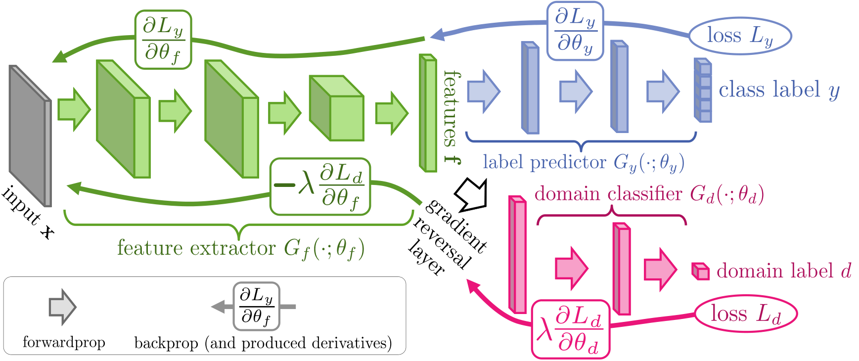
The GRL as defined above is inserted between the feature extractor

G_f

and the domain classifier

G_d

, resulting in the architecture depicted in Figure 10. As the backpropagation process passes through the GRL, the partial derivatives of the loss that is downstream the GRL (i.e./,

{\mathcal{L}}_d

) w.r.t. the layer parameters that are upstream the GRL (i.e./,

{\theta_f}

) get multiplied by

-1

, i.e./,

\frac{\partial {\mathcal{L}}_d}{\partial {\theta_f}}

is effectively replaced with

-\frac{\partial {\mathcal{L}}_d}{\partial {\theta_f}}

. Therefore, running SGD in the resulting model implements the updates of Equations ( Equation 12a- Equation 12c) and converges to a saddle point of Equation 10.

Mathematically, we can formally treat the gradient reversal layer as a "pseudo-function"

{\cal R}({\mathbf x})

defined by two (incompatible) equations describing its forward and backpropagation behaviour:

where

\mathbf{I}

is an identity matrix. We can then define the objective "pseudo-function" of

({\theta_f}, {\theta_y}, {\theta_d})

that is being optimized by the stochastic gradient descent within our method:

\begin{align} &&\tilde E ({\theta_f}, {\theta_y}, {\theta_d}) = \! \frac{1}{n}\sum_{i=1}^n {\mathcal{L}}_y\left(\mathstrut G_y(G_f({\mathbf x}_i; {\theta_f}); {\theta_y}), y_i\right)\\ && - \lambda \, \Big(\frac{1}{n} \sum_{i=1}^{n} {\mathcal{L}}_d \left(\mathstrut G_d({\cal R}(G_f({\mathbf x}_i; {\theta_f})); {\theta_d}), d_i\right) + \frac{1}{n'} \sum_{\mathclap{i=n+1}}^{N} {\mathcal{L}}_d \left(\mathstrut G_d({\cal R}(G_f({\mathbf x}_i; {\theta_f})); {\theta_d}), d_i\right) \Big)\, .\nonumber \end{align}\tag{13}

💭 Click to ask about this equation

Running updates ( Equation 12a- Equation 12c) can then be implemented as doing SGD for ( Equation 13) and leads to the emergence of features that are domain-invariant and discriminative at the same time. After the learning, the label predictor

G_y(G_f({\mathbf x}; {\theta_f}); {\theta_y})

can be used to predict labels for samples from the target domain (as well as from the source domain). Note that we release the source code for the Gradient Reversal layer along with the usage examples as an extension to Caffe ([44]).³

http://sites.skoltech.ru/compvision/projects/grl/

5. Experiments

In this section, we present a variety of empirical results for both shallow domain adversarial neural networks (Subsection 5.1) and deep ones (Subsections 5.2 and 5.3).

5.1 Experiments with Shallow Neural Networks

In this first experiment section, we evaluate the behavior of the simple version of DANN described by Subsection 4.1. Note that the results reported in the present subsection are obtained using Algorithm 1. Thus, the stochastic gradient descent approach here consists of sampling a pair of source and target examples and performing a gradient step update of all parameters of DANN. Crucially, while the update of the regular parameters follows as usual the opposite direction of the gradient, for the adversarial parameters the step must follow the gradient's direction (since we maximize with respect to them, instead of minimizing).

5.1.1 Experiments on a Toy Problem

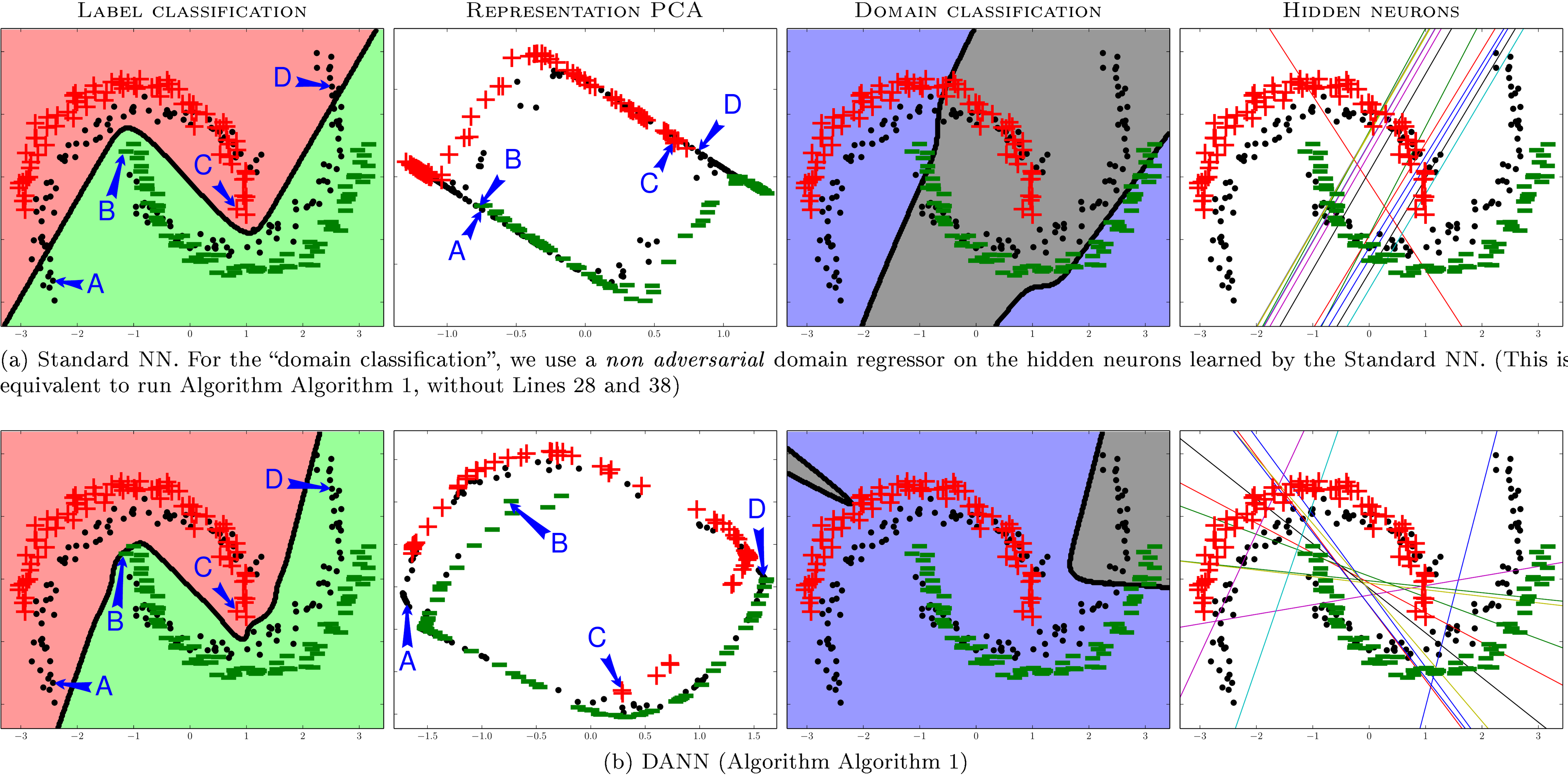
As a first experiment, we study the behavior of the proposed algorithm on a variant of the inter-twinning moons 2D problem, where the target distribution is a rotation of the source one. As the source sample

S

, we generate a lower moon and an upper moon labeled

0

and

1

respectively, each of which containing

150

examples. The target sample

T

is obtained by the following procedure: (1) we generate a sample

S'

the same way

S

has been generated; (2) we rotate each example by

35\degree

; and (3) we remove all the labels. Thus,

T

contains

300

unlabeled examples. We have represented those examples in Figure 1.

We study the adaptation capability of DANN by comparing it to the standard neural network (NN). In these toy experiments, both algorithms share the same network architecture, with a hidden layer size of

15

neurons. We train the NN using the same procedure as the DANN. That is, we keep updating the domain regressor component using target sample

T

(with a hyper-parameter

\lambda=6

; the same value is used for DANN), but we disable the adversarial back-propagation into the hidden layer. To do so, we execute Algorithm 1 by omitting the lines numbered 28 and 38. This allows recovering the NN learning algorithm---based on the source risk minimization of Equation 5 without any regularizer---and simultaneously train the domain regressor of Equation 7 to discriminate between source and target domains. With this toy experience, we will first illustrate how DANN adapts its decision boundary when compared to NN. Moreover, we will also illustrate how the representation given by the hidden layer is less adapted to the source domain task with DANN than with NN (this is why we need a domain regressor in the NN experiment).

We recall that this is the founding idea behind our proposed algorithm.

The analysis of the experiment appears in Figure 1, where upper graphs relate to standard NN, and lower graphs relate to DANN. By looking at the lower and upper graphs pairwise, we compare NN and DANN from four different perspectives, described in details below.

The column "

\text{L{\scriptsize ABEL} C{\scriptsize LASSIFICATION}}

" of Figure 1 shows the decision boundaries of DANN and NN on the problem of predicting the labels of both source and the target examples.

As expected, NN accurately classifies the two classes of the source sample

S

, but is not fully adapted to the target sample

T

. On the contrary, the decision boundary of DANN perfectly classifies examples from both source and target samples. In the studied task, DANN clearly adapts to the target distribution.

The column "

\text{R{\scriptsize EPRESENTATION} P{\scriptsize CA}}

studies how the domain adaptation regularizer affects the representation

G_f(\cdot)

provided by the network hidden layer. The graphs are obtained by applying a Principal component analysis (PCA) on the set of all representation of source and target data points, i.e./,

S(G_f)\cup T(G_f)

. Thus, given the trained network (NN or DANN), every point from

S

and

T

is mapped into a

15

-dimensional feature space through the hidden layer, and projected back into a two-dimensional plane by the PCA transformation.

In the DANN-PCA representation, we observe that target points are homogeneously spread out among source points; In the NN-PCA representation, a number of target points belong to clusters containing no source points. Hence, labeling the target points seems an easier task given the DANN-PCA representation.

To push the analysis further, the PCA graphs tag four crucial data points by the letters A, B, C and D, that correspond to the moon extremities in the original space (note that the original point locations are tagged in the first column graphs). We observe that points A and B are very close to each other in the NN-PCA representation, while they clearly belong to different classes. The same happens to points C and D. Conversely, these four points are at the opposite four corners in the DANN-PCA representation. Note also that the target point A (resp. D)---that is difficult to classify in the original space---is located in the "

\boldsymbol{{+}}

" cluster (resp. "

\boldsymbol{{\pmb{-}}}

" cluster) in the DANN-PCA representation. Therefore, the representation promoted by DANN is better suited to the adaptation problem.

The column "

\text{D{\scriptsize OMAIN} C{\scriptsize LASSIFICATION}}

shows the decision boundary on the domain classification problem, which is given by the domain regressor

G_d

of Equation 7. More precisely, an example

{\mathbf x}

is classified as a source example when

G_d(G_f({\mathbf x}))\geq 0.5

, and is classified as a domain example otherwise. Remember that, during the learning process of DANN, the

G_d

regressor struggles to discriminate between source and target domains, while the hidden representation

G_f(\cdot)

is adversarially updated to prevent it to succeed. As explained above, we trained a domain regressor during the learning process of NN, but without allowing it to influence the learned representation

G_f(\cdot)

On one hand, the DANN domain regressor clearly fails to generalize source and target distribution topologies. On the other hand, the NN domain regressor shows a better (although imperfect) generalization capability. Inter alia, it seems to roughly capture the rotation angle of the target distribution. This again corroborates that the DANN representation does not allow discriminating between domains.

The column "

\text{H{\scriptsize IDDEN} N{\scriptsize EURONS}}

" shows the configuration of hidden layer neurons (by Equation 4, we have that each neuron is indeed a linear regressor). In other words, each of the fifteen plot line corresponds to the coordinates

{\mathbf x}\in {\mathbb{R}}^2

for which the

i

-th component of

G_f({\mathbf x})

equals

\frac{1}{2}

, for

i\in\{1, \ldots, 15\}

We observe that the standard NN neurons are grouped in three clusters, each one allowing to generate a straight line of the zigzag decision boundary for the label classification problem. However, most of these neurons are also able to (roughly) capture the rotation angle of the domain classification problem. Hence, we observe that the adaptation regularizer of DANN prevents these kinds of neurons to be produced. It is indeed striking to see that the two predominant patterns in the NN neurons (i.e./, the two parallel lines crossing the plane from lower left to upper right) are vanishing in the DANN neurons.

5.1.2 Unsupervised Hyper-Parameter Selection

To perform unsupervised domain adaption, one should provide ways to set hyper-parameters (such as the domain regularization parameter

\lambda

, the learning rate, the network architecture for our method) in an unsupervised way, i.e./, without referring to labeled data in the target domain. In the following experiments of Sections 5.1.3 and 5.1.4, we select the hyper-parameters of each algorithm by using a variant of reverse cross-validation approach proposed by [45], that we call reverse validation.

To evaluate the reverse validation risk associated to a tuple of hyper-parameters, we proceed as follows. Given the labeled source sample

S

and the unlabeled target sample

T

, we split each set into training sets (

S'

and

T'

respectively, containing

90\%

of the original examples) and the validation sets (

S_V

and

T_V

respectively). We use the labeled set

S'

and the unlabeled target set

T'

to learn a classifier

\eta

. Then, using the same algorithm, we learn a reverse classifier

\eta_r

using the self-labeled set

\{({\mathbf x}, \eta({\mathbf x}))\}_{{\mathbf x}\in T'}

and the unlabeled part of

S'

as target sample. Finally, the reverse classifier

\eta_r

is evaluated on the validation set

S_V

of source sample. We then say that the classifier

\eta

has a reverse validation risk of

R_{S_V}(\eta_r)

. The process is repeated with multiple values of hyper-parameters and the selected parameters are those corresponding to the classifier with the lowest reverse validation risk.

Note that when we train neural network architectures, the validation set

S_V

is also used as an early stopping criterion during the learning of

\eta

, and self-labeled validation set

\{({\mathbf x}, \eta({\mathbf x}))\}_{{\mathbf x}\in T_V}

is used as an early stopping criterion during the learning of

\eta_r

. We also observed better accuracies when we initialized the learning of the reverse classifier

\eta_r

with the configuration learned by the network

\eta

5.1.3 Experiments on Sentiment Analysis Data Sets

(a) Classification accuracy on the Amazon reviews data set

		Original data			mSDA representation
Source	Target	DANN	NN	SVM	DANN	NN	SVM
books	dvd	.784	.790	.799	.829	.824	.830
books	electronics	.733	.747	.748	.804	.770	.766
books	kitchen	.779	.778	.769	.843	.842	.821

Table 1: Classification accuracy on the Amazon reviews data set, and Pairwise Poisson binomial test.

💭 Click to ask about this table

We now compare the performance of our proposed DANN algorithm to a standard neural network with one hidden layer (NN) described by Equation 5, and a Support Vector Machine (SVM) with a linear kernel.

We compare the algorithms on the Amazon reviews data set, as pre-processed by [7]. This data set includes four domains, each one composed of reviews of a specific kind of product (books, dvd disks, electronics, and kitchen appliances). Reviews are encoded in

5\, 000

dimensional feature vectors of unigrams and bigrams, and labels are binary: "

0

" if the product is ranked up to

3

stars, and "

1

" if the product is ranked

4

5

stars.

We perform twelve domain adaptation tasks.

All learning algorithms are given

2\, 000

labeled source examples and

2\, 000

unlabeled target examples. Then, we evaluate them on separate target test sets (between

3\, 000

and

6\, 000

examples). Note that NN and SVM do not use the unlabeled target sample for learning.

Here are more details about the procedure used for each learning algorithms leading to the empirical results of Table 1.

For the $\text{D{\scriptsize ANN}}$ algorithm, the adaptation parameter $\lambda$ is chosen among 9 values between $10^{-2}$ and $1$ on a logarithmic scale. The hidden layer size $l$ is either $50$ or $100$ . Finally, the learning rate $\mu$ is fixed at $10^{-3}$ .
For the $\text{N{\scriptsize N}}$ algorithm, we use exactly the same hyper-parameters grid and training procedure as DANN above, except that we do not need an adaptation parameter. Note that one can train NN by using the DANN implementation (Algorithm 1) with $\lambda=0$ .
For the $\text{S{\scriptsize VM}}$ algorithm, the hyper-parameter $C$ is chosen among 10 values between $10^{-5}$ and $1$ on a logarithmic scale. This range of values is the same as used by [7] in their experiments.

As presented at Section 5.1.2, we used reverse cross validation selecting the hyper-parameters for all three learning algorithms, with early stopping as the stopping criterion for

\text{D{\scriptsize ANN}}

and

\text{N{\scriptsize N}}

The "Original data" part of Table 1a shows the target test accuracy of all algorithms, and Table 1b reports the probability that one algorithm is significantly better than the others according to the Poisson binomial test ([46]). We note that DANN has a significantly better performance than NN and SVM, with respective probabilities 0.87 and 0.83. As the only difference between DANN and NN is the domain adaptation regularizer, we conclude that our approach successfully helps to find a representation suitable for the target domain.

5.1.4 Combining DANN with Denoising Autoencoders

We now investigate on whether the DANN algorithm can improve on the representation learned by the state-of-the-art Marginalized Stacked Denoising Autoencoders (mSDA) proposed by [7]. In brief, mSDA is an unsupervised algorithm that learns a new robust feature representation of the training samples. It takes the unlabeled parts of both source and target samples to learn a feature map from input space

X

to a new representation space. As a denoising autoencoders algorithm, it finds a feature representation from which one can (approximately) reconstruct the original features of an example from its noisy counterpart.

[7] showed that using mSDA with a linear SVM classifier reaches state-of-the-art performance on the Amazon reviews data sets. As an alternative to the SVM, we propose to apply our Shallow DANN algorithm on the same representations generated by mSDA (using representations of both source and target samples). Note that, even if mSDA and DANN are two representation learning approaches, they optimize different objectives, which can be complementary.

We perform this experiment on the same Amazon reviews data set described in the previous subsection. For each source-target domain pair, we generate the mSDA representations using a corruption probability of

50\%

and a number of layers of

5

. We then execute the three learning algorithms (DANN, NN, and SVM) on these representations. More precisely, following the experimental procedure of [7], we use the concatenation of the output of the

5

layers and the original input as the new representation. Thus, each example is now encoded in a vector of

30\, 000

dimensions. Note that we use the same grid search as in the previous Subsection 5.1.3, but use a learning rate

\mu

10^{-4}

for both DANN and the NN.

The results of "mSDA representation" columns in Table 1a confirm that combining mSDA and DANN is a sound approach. Indeed, the Poisson binomial test shows that DANN has a better performance than the NN and the SVM, with probabilities 0.92 and 0.88 respectively, as reported in Table 1b.

We note however that the standard NN and the SVM find the best solution on respectively the second and the fourth tasks. This suggests that DANN and mSDA adaptation strategies are not fully complementary.

5.1.5 Proxy Distance

The theoretical foundation of the DANN algorithm is the domain adaptation theory of [5,6]. We claimed that DANN finds a representation in which the source and the target example are hardly distinguishable. Our toy experiment of Section 5.1.1 already points out some evidence for that and here we provide analysis on real data. To do so, we compare the Proxy

{\mathcal{A}}

-distance (PAD) on various representations of the Amazon Reviews data set; these representations are obtained by running either NN, DANN, mSDA, or mSDA and DANN combined. Recall that PAD, as described in Section 3.2, is a metric estimating the similarity of the source and the target representations.

More precisely, to obtain a PAD value, we use the following procedure: (1) we construct the data set

U

of Equation 2 using both source and target representations of the training samples; (2) we randomly split

U

in two subsets of equal size; (3) we train linear SVMs on the first subset of

U

using a large range of

C

values; (4) we compute the error of all obtained classifiers on the second subset of

U

; and (5) we use the lowest error to compute the PAD value of Equation 3.

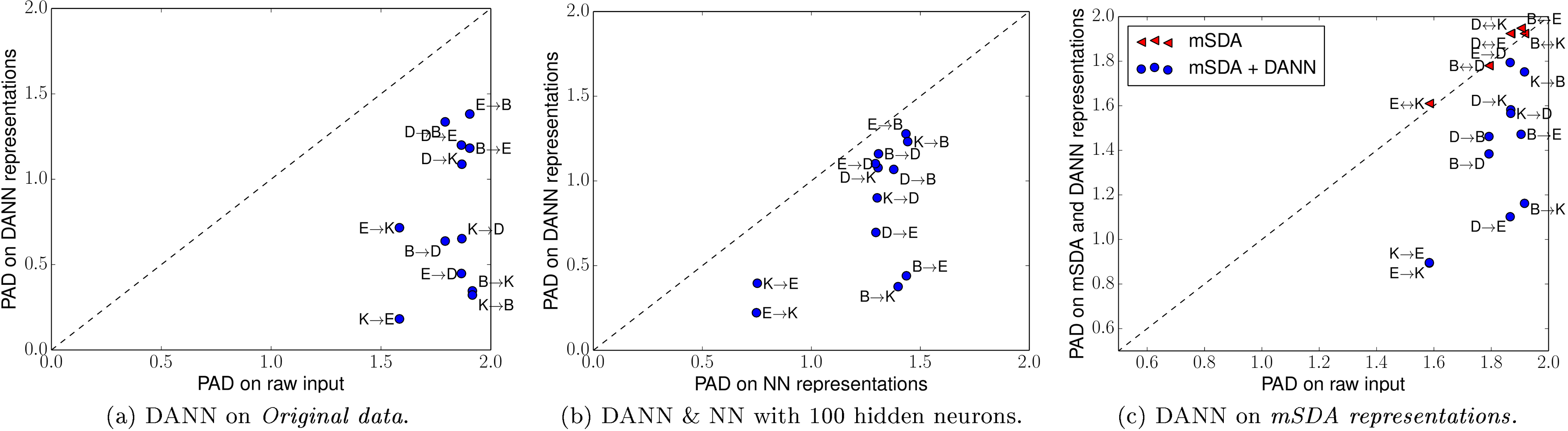
Firstly, Figure 2a compares the PAD of DANN representations obtained in the experiments of Section 5.1.3 (using the hyper-parameters values leading to the results of Table 1) to the PAD computed on raw data. As expected, the PAD values are driven down by the DANN representations.

Secondly, Figure 2b compares the PAD of DANN representations to the PAD of standard NN representations. As the PAD is influenced by the hidden layer size (the discriminating power tends to increase with the representation length), we fix here the size to

100

neurons for both algorithms. We also fix the adaptation parameter of DANN to

\lambda \simeq 0.31

; it was the value that has been selected most of the time during our preceding experiments on the Amazon Reviews data set. Again, DANN is clearly leading to the lowest PAD values.

Lastly, Figure 2c presents two sets of results related to Section 5.1.4 experiments. On one hand, we reproduce the results of [7], which noticed that the mSDA representations have greater PAD values than original (raw) data. Although the mSDA approach clearly helps to adapt to the target task, it seems to contradict the theory of [5]. On the other hand, we observe that, when running DANN on top of mSDA (using the hyper-parameters values leading to the results of Table 1), the obtained representations have much lower PAD values. These observations might explain the improvements provided by DANN when combined with the mSDA procedure.

5.2 Experiments with Deep Networks on Image Classification

We now perform extensive evaluation of a deep version of DANN (see Subsection 4.2) on a number of popular image data sets and their modifications. These include large-scale data sets of small images popular with deep learning methods, and the

\text{O{\scriptsize FFICE}}

data sets ([10]), which are a de facto standard for domain adaptation in computer vision, but have much fewer images.

5.2.1 Baselines

The following baselines are evaluated in the experiments of this subsection. The source-only model is trained without consideration for target-domain data (no domain classifier branch included into the network). The train-on-target model is trained on the target domain with class labels revealed. This model serves as an upper bound on DA methods, assuming that target data are abundant and the shift between the domains is considerable.

In addition, we compare our approach against the recently proposed unsupervised DA method based on subspace alignment (SA) ([26]), which is simple to setup and test on new data sets, but has also been shown to perform very well in experimental comparisons with other "shallow" DA methods. To boost the performance of this baseline, we pick its most important free parameter (the number of principal components) from the range

\{ 2, \ldots, 60 \}

, so that the test performance on the target domain is maximized. To apply SA in our setting, we train a source-only model and then consider the activations of the last hidden layer in the label predictor (before the final linear classifier) as descriptors/features, and learn the mapping between the source and the target domains ([26]).

Since the SA baseline requires training a new classifier after adapting the features, and in order to put all the compared settings on an equal footing, we retrain the last layer of the label predictor using a standard linear SVM ([47]) for all four considered methods (including ours; the performance on the target domain remains approximately the same after the retraining).

For the

\text{O{\scriptsize FFICE}}

data set ([10]), we directly compare the performance of our full network (feature extractor and label predictor) against recent DA approaches using previously published results.

5.2.2 CNN architectures and Training Procedure

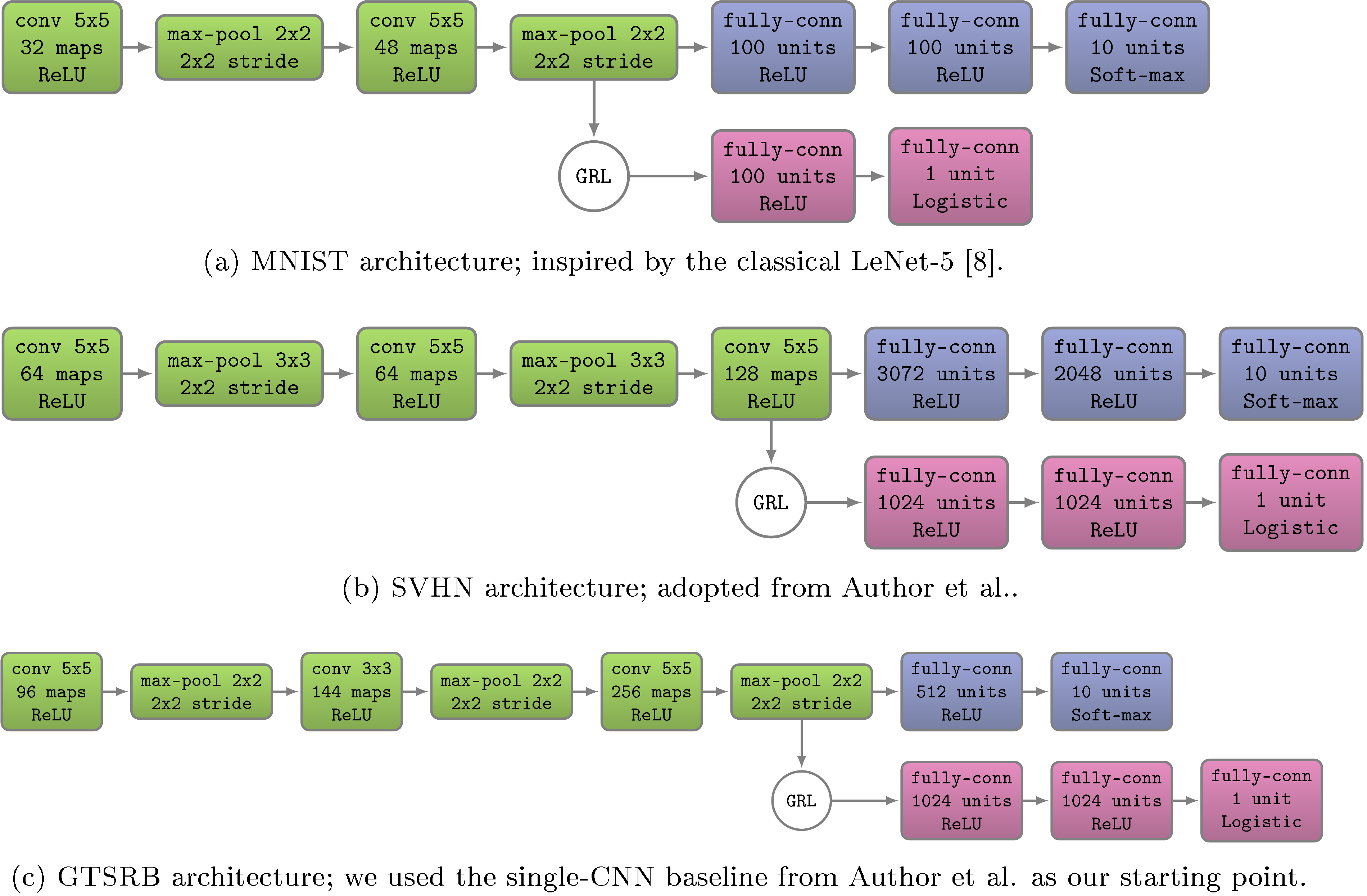
In general, we compose feature extractor from two or three convolutional layers, picking their exact configurations from previous works. More precisely, four different architectures were used in our experiments. The first three are shown in Figure 3. For the

\text{O{\scriptsize FFICE}}

domains, we use pre-trained AlexNet from the Caffe-package ([44]). The adaptation architecture is identical to [32].⁴

A 2-layer domain classifier (

x{\rightarrow}1024{\rightarrow}1024{\rightarrow}2

) is attached to the

256

-dimensional bottleneck of fc7.

For the domain adaption component, we use three (

x{\rightarrow}1024{\rightarrow}1024{\rightarrow}2

) fully connected layers, except for

\text{M{\scriptsize NIST}}

where we used a simpler (

x{\rightarrow}100{\rightarrow}2

) architecture to speed up the experiments. Admittedly these choices for domain classifier are arbitrary, and better adaptation performance might be attained if this part of the architecture is tuned.

For the loss functions, we set

{\mathcal{L}}_y

and

{\mathcal{L}}_d

to be the logistic regression loss and the binomial cross-entropy respectively. Following [48] we also use dropout and

\ell_2

-norm restriction when we train the SVHN architecture.

The other hyper-parameters are not selected through a grid search as in the small scale experiments of Section 5.1, which would be computationally costly. Instead, the learning rate is adjusted during the stochastic gradient descent using the following formula:

where

p

is the training progress linearly changing from 0 to 1,

\mu_0 = 0.01

\alpha = 10

and

\beta = 0.75

(the schedule was optimized to promote convergence and low error on the source domain). A momentum term of

0.9

is also used.

The domain adaptation parameter

\lambda

is initiated at

0

and is gradually changed to

1

using the following schedule:

where

\gamma

was set to

10

in all experiments (the schedule was not optimized/tweaked). This strategy allows the domain classifier to be less sensitive to noisy signal at the early stages of the training procedure. Note however that these

\lambda_p

were used only for updating the feature extractor component

G_f

. For updating the domain classification component, we used a fixed

\lambda=1

, to ensure that the latter trains as fast as the label predictor

G_y

.⁵

Equivalently, one can use the same

\lambda_p

for both feature extractor and domain classification components, but use a learning rate of

\mu/\lambda_p

for the latter.

Finally, note that the model is trained on

128

-sized batches (images are preprocessed by the mean subtraction). A half of each batch is populated by the samples from the source domain (with known labels), the rest constitutes the target domain (with labels not revealed to the algorithms except for the train-on-target baseline).

5.2.3 Visualizations

💭 Click to ask about this figure

We use t-SNE ([49]) projection to visualize feature distributions at different points of the network, while color-coding the domains (Figure 4). As we already observed with the shallow version of DANN (see Figure 1), there is a strong correspondence between the success of the adaptation in terms of the classification accuracy for the target domain, and the overlap between the domain distributions in such visualizations.

5.2.4 Results On Image Data Sets

Table 2: Classification accuracies for digit image classifications for different source and target domains. $\text{M{\scriptsize NIST-M}}$ corresponds to difference-blended digits over non-uniform background. The first row corresponds to the lower performance bound (i.e., if no adaptation is performed). The last row corresponds to training on the target domain data with known class labels (upper bound on the DA performance). For each of the two DA methods (ours and [26]) we show how much of the gap between the lower and the upper bounds was covered (in brackets). For all five cases, our approach outperforms [26] considerably, and covers a big portion of the gap.

Method	Source	MNIST	Syn Numbers	SVHN	Syn Signs
Method	Target	MNIST-M	SVHN	MNIST	GTSRB
Source only		$.5225$	$.8674$	$.5490$	$.7900$
SA ([26])		$.5690 \; (4.1\%)$	$.8644 \; (-5.5\%)$	$.5932 \; (9.9\%)$	$.8165 \; (12.7\%)$
DANN		$\mathbf{.7666} \; (52.9\%)$	$\mathbf{.9109} \; (79.7\%)$	$\mathbf{.7385} \; (42.6\%)$	$\mathbf{.8865} \; (46.4\%)$
Train on target		$.9596$	$.9220$	$.9942$	$.9980$

Table 3: Accuracy evaluation of different DA approaches on the standard $\text{O{\scriptsize FFICE}}$ ([10]) data set. All methods (except SA) are evaluated in the ``fully-transductive'' protocol (some results are reproduced from [33]). Our method (last row) outperforms competitors setting the new state-of-the-art.

Method	Source	Amazon	DSLR	Webcam
Method	Target	Webcam	Webcam	DSLR
GFK(PLS, PCA) ([25])		$.197$	$.497$	$.6631$
SA* ([26])		$.450$	$.648$	$.699$
DLID ([27])		$.519$	$.782$	$.899$

We now discuss the experimental settings and the results. In each case, we train on the source data set and test on a different target domain data set, with considerable shifts between domains (see Figure 5). The results are summarized in Table 2 and Table 3.

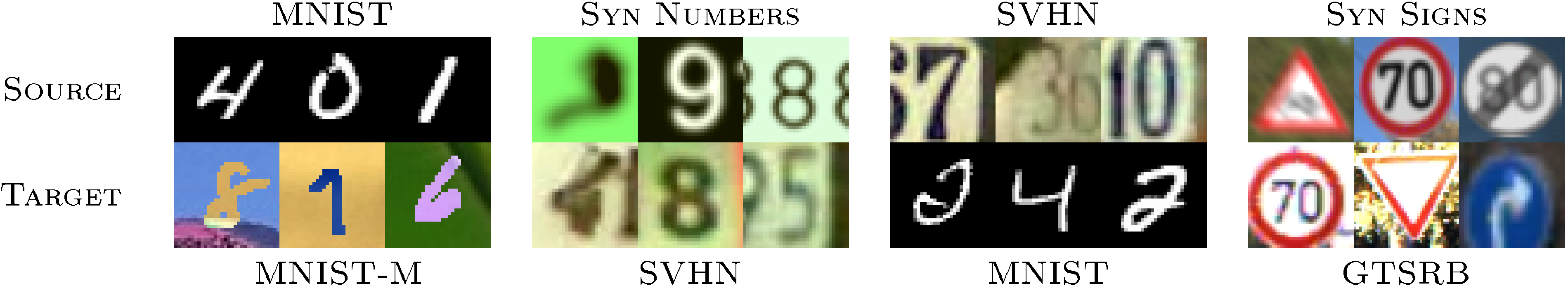
MNIST $\rightarrow$ MNIST-M.

Our first experiment deals with the MNIST data set ([8]) (source). In order to obtain the target domain (

\text{M{\scriptsize NIST-M}}

) we blend digits from the original set over patches randomly extracted from color photos from BSDS500 ([50]). This operation is formally defined for two images

I^{1}, I^{2}

I_{ijk}^{out} = | I_{ijk}^{1} - I_{ijk}^{2} |

, where

i, j

are the coordinates of a pixel and

k

is a channel index. In other words, an output sample is produced by taking a patch from a photo and inverting its pixels at positions corresponding to the pixels of a digit. For a human the classification task becomes only slightly harder compared to the original data set (the digits are still clearly distinguishable) whereas for a CNN trained on MNIST this domain is quite distinct, as the background and the strokes are no longer constant. Consequently, the source-only model performs poorly. Our approach succeeded at aligning feature distributions (Figure 4), which led to successful adaptation results (considering that the adaptation is unsupervised). At the same time, the improvement over source-only model achieved by subspace alignment (SA) ([26]) is quite modest, thus highlighting the difficulty of the adaptation task.

Synthetic numbers $\rightarrow$ SVHN.

To address a common scenario of training on synthetic data and testing on real data, we use Street-View House Number data set

\text{S{\scriptsize VHN}}

([9]) as the target domain and synthetic digits as the source. The latter (

\text{S{\scriptsize YN} N{\scriptsize UMBERS}}

) consists of

\approx 500, 000

images generated by ourselves from Windows

^{\text{TM}}

fonts by varying the text (that includes different one-, two-, and three-digit numbers), positioning, orientation, background and stroke colors, and the amount of blur. The degrees of variation were chosen manually to simulate

\text{S{\scriptsize VHN}}

, however the two data sets are still rather distinct, the biggest difference being the structured clutter in the background of

\text{S{\scriptsize VHN}}

images.

The proposed backpropagation-based technique works well covering almost 80% of the gap between training with source data only and training on target domain data with known target labels. In contrast, SA ([26]) results in a slight classification accuracy drop (probably due to the information loss during the dimensionality reduction), indicating that the adaptation task is even more challenging than in the case of the

\text{M{\scriptsize NIST}}

experiment.

MNIST $\leftrightarrow$ SVHN.

In this experiment, we further increase the gap between distributions, and test on

\text{M{\scriptsize NIST}}

and

\text{S{\scriptsize VHN}}

, which are significantly different in appearance. Training on SVHN even without adaptation is challenging --- classification error stays high during the first 150 epochs. In order to avoid ending up in a poor local minimum we, therefore, do not use learning rate annealing here. Obviously, the two directions (

\text{M{\scriptsize NIST}}

\rightarrow

\text{S{\scriptsize VHN}}

and

\text{S{\scriptsize VHN}}

\rightarrow

\text{M{\scriptsize NIST}}

) are not equally difficult. As

\text{S{\scriptsize VHN}}

is more diverse, a model trained on SVHN is expected to be more generic and to perform reasonably on the MNIST data set. This, indeed, turns out to be the case and is supported by the appearance of the feature distributions. We observe a quite strong separation between the domains when we feed them into the CNN trained solely on

\text{M{\scriptsize NIST}}

, whereas for the

\text{S{\scriptsize VHN}}

-trained network the features are much more intermixed. This difference probably explains why our method succeeded in improving the performance by adaptation in the

\text{S{\scriptsize VHN}}

\rightarrow

\text{M{\scriptsize NIST}}

scenario (see Table 2) but not in the opposite direction (SA is not able to perform adaptation in this case either). Unsupervised adaptation from

\text{M{\scriptsize NIST}}

\text{S{\scriptsize VHN}}

gives a failure example for our approach: it doesn't manage to improve upon the performance of the non-adapted model which achieves

\approx 0.25

accuracy (we are unaware of any unsupervised DA methods capable of performing such adaptation).

Synthetic Signs $\rightarrow$ GTSRB.

Overall, this setting is similar to the

\text{S{\scriptsize YN} N{\scriptsize UMBERS}}

\rightarrow

\text{S{\scriptsize VHN}}

experiment, except the distribution of the features is more complex due to the significantly larger number of classes (43 instead of 10). For the source domain we obtained

100, 000

synthetic images (which we call

\text{S{\scriptsize YN} S{\scriptsize IGNS}}

) simulating various imaging conditions. In the target domain, we use

31, 367

random training samples for unsupervised adaptation and the rest for evaluation. Once again, our method achieves a sensible increase in performance proving its suitability for the synthetic-to-real data adaptation.

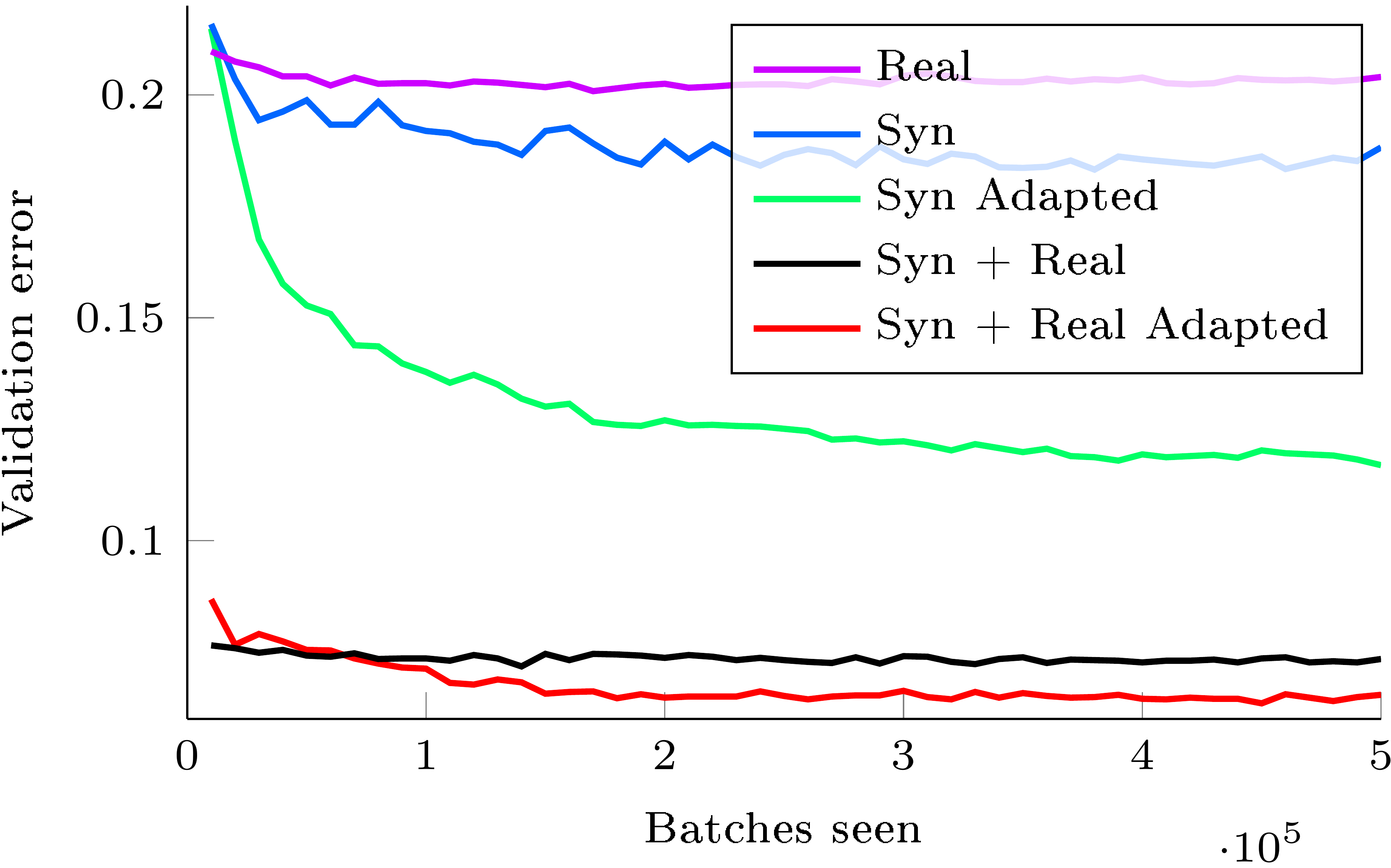
As an additional experiment, we also evaluate the proposed algorithm for semi-supervised domain adaptation, i.e./, when one is additionally provided with a small amount of labeled target data. Here, we reveal

430

labeled examples (10 samples per class) and add them to the training set for the label predictor. Figure 6 shows the change of the validation error throughout the training. While the graph clearly suggests that our method can be beneficial in the semi-supervised setting, thorough verification of semi-supervised setting is left for future work.

Office data set. We finally evaluate our method on

\text{O{\scriptsize FFICE}}

data set, which is a collection of three distinct domains:

\text{A{\scriptsize MAZON}}

\text{D{\scriptsize SLR}}

, and

\text{W{\scriptsize EBCAM}}

. Unlike previously discussed data sets,

\text{O{\scriptsize FFICE}}

is rather small-scale with only 2817 labeled images spread across 31 different categories in the largest domain. The amount of available data is crucial for a successful training of a deep model, hence we opted for the fine-tuning of the CNN pre-trained on the ImageNet (AlexNet from the Caffe package, see [44]) as it is done in some recent DA works ([51,32,52,33]). We make our approach more comparable with [32] by using exactly the same network architecture replacing domain mean-based regularization with the domain classifier.

Following previous works, we assess the performance of our method across three transfer tasks most commonly used for evaluation. Our training protocol is adopted from [22,27,33] as during adaptation we use all available labeled source examples and unlabeled target examples (the premise of our method is the abundance of unlabeled data in the target domain). Also, all source domain data are used for training. Under this "fully-transductive" setting, our method is able to improve previously-reported state-of-the-art accuracy for unsupervised adaptation very considerably (Table 3), especially in the most challenging

\text{A{\scriptsize MAZON}}

\rightarrow

\text{W{\scriptsize EBCAM}}

scenario (the two domains with the largest domain shift).

Interestingly, in all three experiments we observe a slight over-fitting (performance on the target domain degrades while accuracy on the source continues to improve) as training progresses, however, it doesn't ruin the validation accuracy. Moreover, switching off the domain classifier branch makes this effect far more apparent, from which we conclude that our technique serves as a regularizer.

5.3 Experiments with Deep Image Descriptors for Re-Identification

In this section we discuss the application of the described adaptation method to person re-identification (re-id) problem. The task of person re-identification is to associate people seen from different camera views. More formally, it can be defined as follows: given two sets of images from different cameras (probe and gallery) such that each person depicted in the probe set has an image in the gallery set, for each image of a person from the probe set find an image of the same person in the gallery set. Disjoint camera views, different illumination conditions, various poses and low quality of data make this problem difficult even for humans (e.g./, [53], reports human performance at Rank1=

71.08\%

Unlike classification problems that are discussed above, re-identification problem implies that each image is mapped to a vector descriptor. The distance between descriptors is then used to match images from the probe set and the gallery set. To evaluate results of re-id methods the Cumulative Match Characteristic (CMC) curve is commonly used. It is a plot of the identification rate (recall) at rank-

k

, that is the probability of the matching gallery image to be within the closest

k

images (in terms of descriptor distance) to the probe image.

Most existing works train descriptor mappings and evaluate them within the same data set containing images from a certain camera network with similar imaging conditions. Several papers, however, observed that the performance of the resulting re-identification systems drops very considerably when descriptors trained on one data set and tested on another. It is therefore natural to handle such cross-domain evaluation as a domain-adaptation problem, where each camera network (data set) constitutes a domain.

Recently, several papers with significantly improved re-identification performance ([54,55,56]) have been presented, with [57] reporting good results in cross-data-set evaluation scenario. At the moment, deep learning methods ([58]) do not achieve state-of-the-art results probably because of the limited size of the training sets. Domain adaptation thus represents a viable direction for improving deep re-identification descriptors.

5.3.1 Data Sets and Protocols

Following [57], we use PRID ([59]), VIPeR ([60]), CUHK ([61]) as target data sets for our experiments. The PRID data set exists in two versions, and as in [57] we use a single-shot variant. It contains images of

385

persons viewed from camera A and images of

749

persons viewed from camera B,

200

persons appear in both cameras. The VIPeR data set also contains images taken with two cameras, and in total

632

persons are captured, for every person there is one image for each of the two camera views. The CUHK data set consists of images from five pairs of cameras, two images for each person from each of the two cameras. We refer to the subset of this data set that includes the first pair of cameras only as CUHK/p1 (as most papers use this subset). See Figure 7 for samples of these data sets.

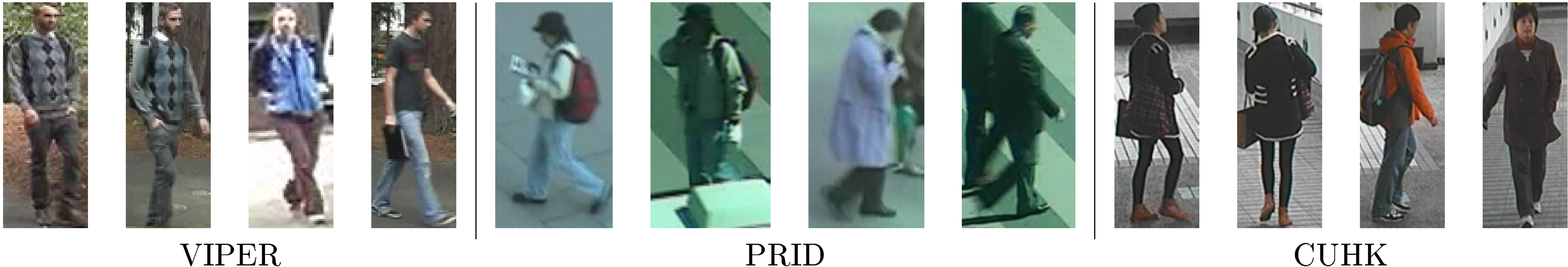
We perform extensive experiments for various pairs of data sets, where one data set serves as a source domain, i.e./, it is used to train a descriptor mapping in a supervised way with known correspondences between probe and gallery images. The second data set is used as a target domain, so that images from that data set are used without probe-gallery correspondence.

In more detail, CUHK/p1 is used for experiments when CUHK serves as a target domain and two settings ("whole CUHK" and CUHK/p1) are used for experiments when CUHK serves as a source domain. Given PRID as a target data set, we randomly choose 100 persons appearing in both camera views as training set. The images of the other 100 persons from camera A are used as probe, all images from camera B excluding those used in training (649 in total) are used as gallery at test time. For VIPeR, we use random 316 persons for training and all others for testing. For CUHK, 971 persons are split into 485 for training and 486 for testing. Unlike [57], we use all images in the first pair of cameras of CUHK instead of choosing one image of a person from each camera view. We also performed two experiments with all images of the whole CUHK data set as source domain and VIPeR and PRID data sets as target domains as in the original paper ([58]).

Following [58], we augmented our data with mirror images, and during test time we calculate similarity score between two images as the mean of the four scores corresponding to different flips of the two compared images. In case of CUHK, where there are 4 images (including mirror images) for each of the two camera views for each person, all 16 combinations' scores are averaged.

5.3.2 CNN architectures and Training Procedure

In our experiments, we use siamese architecture described in [58] (Deep Metric Learning or DML) for learning deep image descriptors on the source data set. This architecture incorporates two convolution layers (with

7\times7

and

5\times5

filter banks), followed by ReLU and max pooling, and one fully-connected layer, which gives

500

-dimensional descriptors as an output. There are three parallel flows within the CNN for processing three part of an image: the upper, the middle, and the lower one. The first convolution layer shares parameters between three parts, and the outputs of the second convolution layers are concatenated. During training, we follow [58] and calculate pairwise cosine similarities between

500

-dimensional features within each batch and backpropagate the loss for all pairs within batch.

To perform domain-adversarial training, we construct a DANN architecture. The feature extractor includes the two convolutional layers (followed by max-pooling and ReLU) discussed above. The label predictor in this case is replaced with descriptor predictor that includes one fully-connected layer. The domain classifier includes two fully-connected layers with

500

units in the intermediate representation (

x{\rightarrow}500{\rightarrow}1

For the verification loss function in the descriptor predictor we used Binomial Deviance loss, defined in [58] with similar parameters:

\alpha = 2

\beta = 0.5

c = 2

(the asymmetric cost parameter for negative pairs). The domain classifier is trained with logistic loss as in subsection 5.2.2.

We used learning rate fixed to

0.001

and momentum of

0.9

. The schedule of adaptation similar to the one described in subsection 5.2.2 was used. We also inserted dropout layer with rate

0.5

after the concatenation of outputs of the second max-pooling layer.

128

-sized batches were used for source data and

128

-sized batches for target data.

5.3.3 Results on Re-identification data sets

Figure 8 shows results in the form of CMC-curves for eight pairs of data sets. Depending on the hardness of the annotation problem we trained either for 50, 000 iterations (CUHK/p1

\rightarrow

VIPeR, VIPeR

\rightarrow

CUHK/p1, PRID

\rightarrow

VIPeR) or for 20, 000 iterations (the other five pairs).

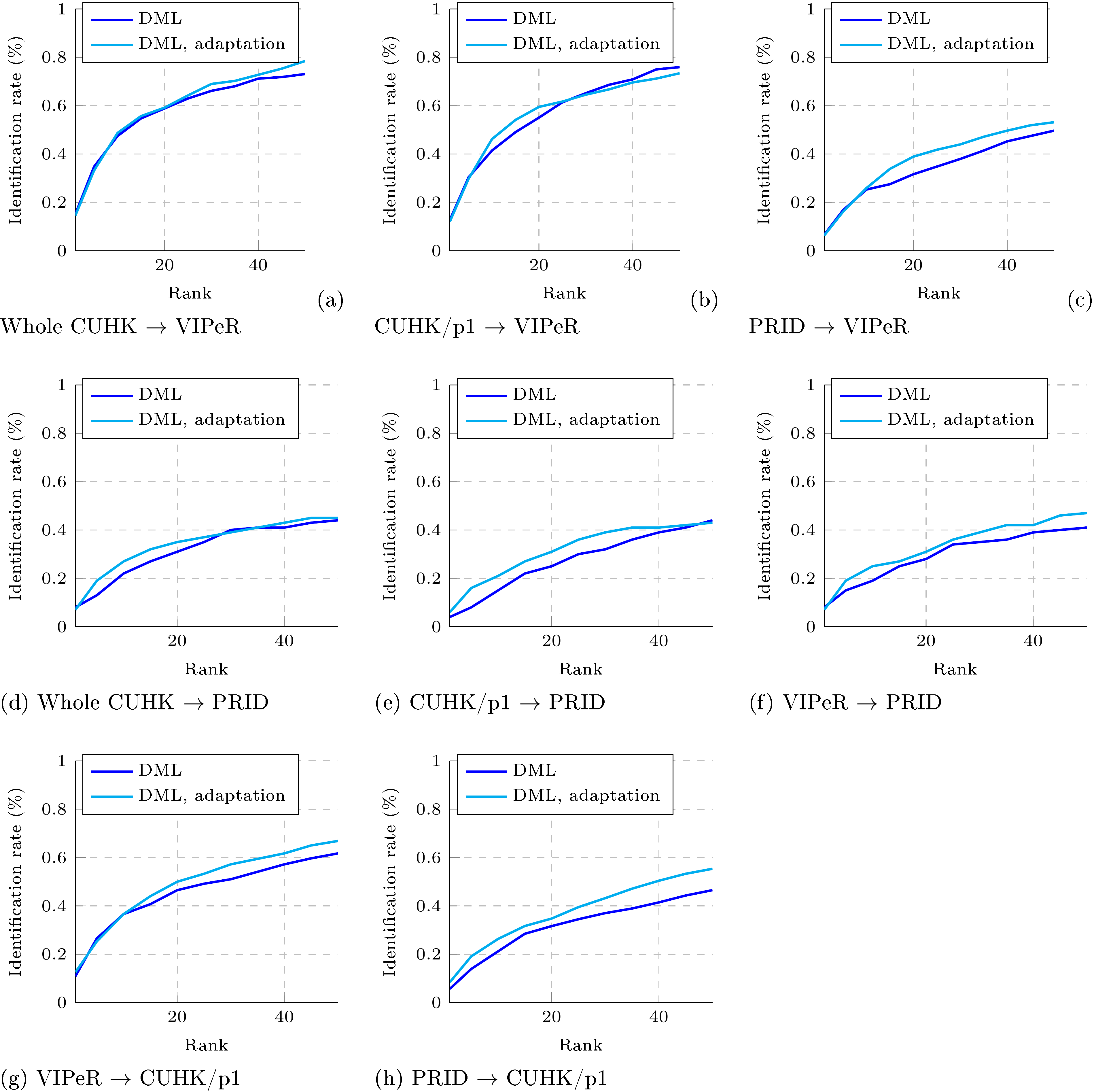
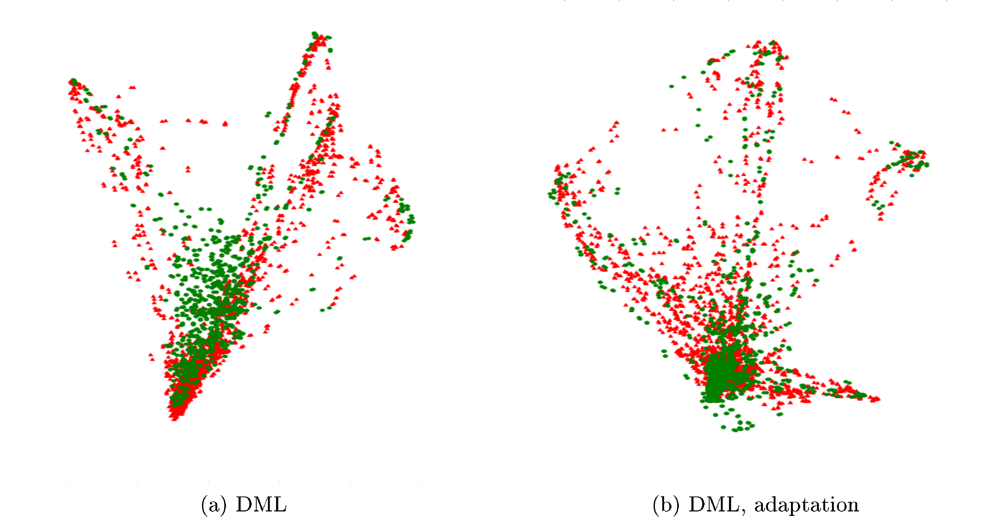
After the sufficient number of iterations, domain-adversarial training consistently improves the performance of re-identification. For the pairs that involve PRID data set, which is more dissimilar to the other two data sets, the improvement is considerable. Overall, this demonstrates the applicability of the domain-adversarial learning beyond classification problems.

Figure 9 further demonstrates the effect of adaptation on the distributions of the learned descriptors in the source and in target sets in VIPeR

\rightarrow

CUHK/p1 experiments, where domain adversarial learning once again achieves better intermixing of the two domains.

6. Conclusion

The paper proposes a new approach to domain adaptation of feed-forward neural networks, which allows large-scale training based on large amount of annotated data in the source domain and large amount of unannotated data in the target domain. Similarly to many previous shallow and deep DA techniques, the adaptation is achieved through aligning the distributions of features across the two domains. However, unlike previous approaches, the alignment is accomplished through standard backpropagation training.

The approach is motivated and supported by the domain adaptation theory of [5,6]. The main idea behind DANN is to enjoin the network hidden layer to learn a representation which is predictive of the source example labels, but uninformative about the domain of the input (source or target). We implement this new approach within both shallow and deep feed-forward architectures. The latter allows simple implementation within virtually any deep learning package through the introduction of a simple gradient reversal layer. We have shown that our approach is flexible and achieves state-of-the-art results on a variety of benchmark in domain adaptation, namely for sentiment analysis and image classification tasks.

A convenient aspect of our approach is that the domain adaptation component can be added to almost any neural network architecture that is trainable with backpropagation. Towards this end, We have demonstrated experimentally that the approach is not confined to classification tasks but can be used in other feed-forward architectures, e.g./, for descriptor learning for person re-identification.

7. Acknowledgments

This work has been supported by National Science and Engineering Research Council (NSERC) Discovery grants 262067 and 0122405 as well as the Russian Ministry of Science and Education grant RFMEFI57914X0071. Computations were performed on the Colosse supercomputer grid at Université Laval, under the auspices of Calcul Québec and Compute Canada. The operations of Colosse are funded by the NSERC, the Canada Foundation for Innovation (CFI), NanoQuébec, and the Fonds de recherche du Québec -- Nature et technologies (FRQNT). We also thank the Graphics & Media Lab, Faculty of Computational Mathematics and Cybernetics, Lomonosov Moscow State University for providing the synthetic road signs data set.

References

[1] Joerg Liebelt and Cordelia Schmid. Multi-view object class detection with a 3d geometric model. In CVPR, 2010.

[2] Michael Stark, Michael Goesele, and Bernt Schiele. Back to the future: Learning shape models from 3d CAD data. In BMVC, pages 1–11, 2010.

[3] David V{'a}zquez, Antonio Manuel L{'o}pez, Javier Mar{'\i}n, Daniel Ponsa, and David Ger{'o}nimo Gomez. Virtual and real world adaptationfor pedestrian detection. IEEE Transaction Pattern Analysis and Machine Intelligence, 36(4):797–809, 2014.

[4] Baochen Sun and Kate Saenko. From virtual to reality: Fast adaptation of virtual object detectors to real domains. In BMVC, 2014.

[5] Shai Ben-David, John Blitzer, Koby Crammer, and Fernando Pereira. Analysis of representations for domain adaptation. In NIPS, pages 137–144, 2006.

[6] Shai Ben-David, John Blitzer, Koby Crammer, Alex Kulesza, Fernando Pereira, and Jennifer Wortman Vaughan. A theory of learning from different domains. Machine Learning, 79(1-2):151–175, 2010.

[7] Minmin Chen, Zhixiang Eddie Xu, Kilian Q. Weinberger, and Fei Sha. Marginalized denoising autoencoders for domain adaptation. In ICML, pages 767–774, 2012.

[8] Y. LeCun, L. Bottou, Y. Bengio, and P. Haffner. Gradient-based learning applied to document recognition. Proceedings of the IEEE, 86(11):2278–2324, November 1998.

[9] Yuval Netzer, Tao Wang, Adam Coates, Alessandro Bissacco, Bo Wu, and Andrew Y. Ng. Reading digits in natural images with unsupervised feature learning. In NIPS Workshop on Deep Learning and Unsupervised Feature Learning, 2011.

[10] Kate Saenko, Brian Kulis, Mario Fritz, and Trevor Darrell. Adapting visual category models to new domains. In ECCV, pages 213–226, 2010.

[11] Shaogang Gong, Marco Cristani, Shuicheng Yan, and Chen Change Loy. Person re-identification. Springer, 2014.

[12] John Blitzer, Ryan T. McDonald, and Fernando Pereira. Domain adaptation with structural correspondence learning. In Conference on Empirical Methods in Natural Language Processing, pages 120–128, 2006.

[13] Lorenzo Bruzzone and Mattia Marconcini. Domain adaptation problems: A DASVM classification technique and a circular validation strategy. IEEE Transaction Pattern Analysis and Machine Intelligence, 32(5):770–787, 2010.

[14] Pascal Germain, Amaury Habrard, François Laviolette, and Emilie Morvant. A PAC-Bayesian approach for domain adaptation with specialization to linear classifiers. In ICML, pages 738–746, 2013.

[15] Mahsa Baktashmotlagh, Mehrtash Tafazzoli Harandi, Brian C. Lovell, and Mathieu Salzmann. Unsupervised domain adaptation by domain invariant projection. In ICCV, pages 769–776, 2013.

[16] Corinna Cortes and Mehryar Mohri. Domain adaptation and sample bias correction theory and algorithm for regression. Theor. Comput. Sci., 519:103–126, 2014.

[17] Xavier Glorot, Antoine Bordes, and Yoshua Bengio. Domain adaptation for large-scale sentiment classification: A deep learning approach. In ICML, pages 513–520, 2011.

[18] Yujia Li, Kevin Swersky, and Richard Zemel. Unsupervised domain adaptation by domain invariant projection. In NIPS 2014 Workshop on Transfer and Multitask Learning, 2014.

[19] Pascal Vincent, Hugo Larochelle, Yoshua Bengio, and Pierre-Antoine Manzagol. Extracting and composing robust features with denoising autoencoders. In ICML, pages 1096–1103, 2008.

[20] Karsten M. Borgwardt, Arthur Gretton, Malte J. Rasch, Hans-Peter Kriegel, Bernhard Schölkopf, and Alexander J. Smola. Integrating structured biological data by kernel maximum mean discrepancy. In ISMB, pages 49–57, 2006.

[21] Jiayuan Huang, Alexander J. Smola, Arthur Gretton, Karsten M. Borgwardt, and Bernhard Schölkopf. Correcting sample selection bias by unlabeled data. In NIPS, pages 601–608, 2006.

[22] Boqing Gong, Kristen Grauman, and Fei Sha. Connecting the dots with landmarks: Discriminatively learning domain-invariant features for unsupervised domain adaptation. In ICML, pages 222–230, 2013.

[23] Sinno Jialin Pan, Ivor W. Tsang, James T. Kwok, and Qiang Yang. Domain adaptation via transfer component analysis. IEEE Transactions on Neural Networks, 22(2):199–210, 2011.

[24] Raghuraman Gopalan, Ruonan Li, and Rama Chellappa. Domain adaptation for object recognition: An unsupervised approach. In ICCV, pages 999–1006, 2011.

[25] Boqing Gong, Yuan Shi, Fei Sha, and Kristen Grauman. Geodesic flow kernel for unsupervised domain adaptation. In CVPR, pages 2066–2073, 2012.

[26] Basura Fernando, Amaury Habrard, Marc Sebban, and Tinne Tuytelaars. Unsupervised visual domain adaptation using subspace alignment. In ICCV, 2013.

[27] S. Chopra, S. Balakrishnan, and R. Gopalan. Dlid: Deep learning for domain adaptation by interpolating between domains. In ICML Workshop on Challenges in Representation Learning, 2013.

[28] Matthew D. Zeiler and Rob Fergus. Visualizing and understanding convolutional networks. CoRR, abs/1311.2901, 2013. URL http://arxiv.org/abs/1311.2901

[29] M. Oquab, L. Bottou, I. Laptev, and J. Sivic. Learning and transferring mid-level image representations using convolutional neural networks. In CVPR, 2014.

[30] Artem Babenko, Anton Slesarev, Alexander Chigorin, and Victor S. Lempitsky. Neural codes for image retrieval. In ECCV, pages 584–599, 2014.

[31] Ian Goodfellow, Jean Pouget-Abadie, Mehdi Mirza, Bing Xu, David Warde-Farley, Sherjil Ozair, Aaron Courville, and Yoshua Bengio. Generative adversarial nets. In NIPS, 2014.

[32] Eric Tzeng, Judy Hoffman, Ning Zhang, Kate Saenko, and Trevor Darrell. Deep domain confusion: Maximizing for domain invariance. CoRR, abs/1412.3474, 2014. URL http://arxiv.org/abs/1412.3474

[33] Mingsheng Long and Jianmin Wang. Learning transferable features with deep adaptation networks. CoRR, abs/1502.02791, 2015.

[34] Qiang Chen, Junshi Huang, Rogerio Feris, Lisa M. Brown, Jian Dong, and Shuicheng Yan. Deep domain adaptation for describing people based on fine-grained clothing attributes. In CVPR, June 2015.

[35] Fei Huang and Alexander Yates. Biased representation learning for domain adaptation. In Joint Conference on Empirical Methods in Natural Language Processing and Computational Natural Language Learning, pages 1313–1323, 2012.

[36] Yaroslav Ganin and Victor Lempitsky. Unsupervised domain adaptation by backpropagation. In ICML, pages 325–333, 2015. URL http://jmlr.org/proceedings/papers/v37/ganin15.html

[37] Hana Ajakan, Pascal Germain, Hugo Larochelle, François Laviolette, and Mario Marchand. Domain-adversarial neural networks. NIPS 2014 Workshop on Transfer and Multi-task learning: Theory Meets Practice, 2014. URL http://arxiv.org/abs/1412.4446

[38] Yishay Mansour, Mehryar Mohri, and Afshin Rostamizadeh. Domain adaptation: Learning bounds and algorithms. In COLT, 2009a.

[39] Yishay Mansour, Mehryar Mohri, and Afshin Rostamizadeh. Multiple source adaptation and the r{'e}nyi divergence. In UAI, pages 367–374, 2009b.

[40] Daniel Kifer, Shai Ben-David, and Johannes Gehrke. Detecting change in data streams. In Very Large Data Bases, pages 180–191, 2004.

[41] Alex Krizhevsky, Ilya Sutskever, and Geoffrey Hinton. Imagenet classification with deep convolutional neural networks. In NIPS, pages 1097–1105, 2012.

[42] John Duchi, Elad Hazan, and Yoram Singer. Adaptive subgradient methods for online learning and stochastic optimization. Technical report, EECS Department, University of California, Berkeley, Mar 2010.

[43] Matthew D. Zeiler. ADADELTA: an adaptive learning rate method. CoRR, abs/1212.5701, 2012. URL http://arxiv.org/abs/1212.5701

[44] Yangqing Jia, Evan Shelhamer, Jeff Donahue, Sergey Karayev, Jonathan Long, Ross Girshick, Sergio Guadarrama, and Trevor Darrell. Caffe: Convolutional architecture for fast feature embedding. CoRR, abs/1408.5093, 2014.

[45] Erheng Zhong, Wei Fan, Qiang Yang, Olivier Verscheure, and Jiangtao Ren. Cross validation framework to choose amongst models and datasets for transfer learning. In Machine Learning and Knowledge Discovery in Databases, pages 547–562. Springer, 2010.

[46] Alexandre Lacoste, François Laviolette, and Mario Marchand. Bayesian comparison of machine learning algorithms on single and multiple datasets. In AISTATS, pages 665–675, 2012.

[47] Rong-En Fan, Kai-Wei Chang, Cho-Jui Hsieh, Xiang-Rui Wang, and Chih-Jen Lin. LIBLINEAR: A library for large linear classification. Journal of Machine Learning Research, 9:1871–1874, 2008.

[48] Nitish Srivastava, Geoffrey Hinton, Alex Krizhevsky, Ilya Sutskever, and Ruslan Salakhutdinov. Dropout: A simple way to prevent neural networks from overfitting. The Journal of Machine Learning Research, 15(1):1929–1958, 2014.

[49] Laurens van der Maaten. Barnes-Hut-SNE. CoRR, abs/1301.3342, 2013. URL http://arxiv.org/abs/1301.3342

[50] Pablo Arbelaez, Michael Maire, Charless Fowlkes, and Jitendra Malik. Contour detection and hierarchical image segmentation. IEEE Transaction Pattern Analysis and Machine Intelligence, 33, 2011.

[51] Jeff Donahue, Yangqing Jia, Oriol Vinyals, Judy Hoffman, Ning Zhang, Eric Tzeng, and Trevor Darrell. Decaf: A deep convolutional activation feature for generic visual recognition. In ICML, 2014.

[52] Judy Hoffman, Eric Tzeng, Jeff Donahue, Yangqing Jia, Kate Saenko, and Trevor Darrell. One-shot adaptation of supervised deep convolutional models. CoRR, abs/1312.6204, 2013. URL http://arxiv.org/abs/1312.6204

[53] Chunxiao Liu, Chen Change Loy, Shaogang Gong, and Guijin Wang. POP: person re-identification post-rank optimisation. In ICCV, pages 441–448, 2013.

[54] Ziming Zhang and Venkatesh Saligrama. Person re-identification via structured prediction. CoRR, abs/1406.4444, 2014. URL http://arxiv.org/abs/1406.4444

[55] Rui Zhao, Wanli Ouyang, and Xiaogang Wang. Person re-identification by saliency learning. CoRR, abs/1412.1908, 2014. URL http://arxiv.org/abs/1412.1908

[56] Sakrapee Paisitkriangkrai, Chunhua Shen, and Anton van den Hengel. Learning to rank in person re-identification with metric ensembles. CoRR, abs/1503.01543, 2015. URL http://arxiv.org/abs/1503.01543

[57] Andy Jinhua Ma, Jiawei Li, Pong C. Yuen, and Ping Li. Cross-domain person reidentification using domain adaptation ranking svms. IEEE Transactions on Image Processing, 24(5):1599–1613, 2015.

[58] Dong Yi, Zhen Lei, and Stan Z. Li. Deep metric learning for practical person re-identification. CoRR, abs/1407.4979, 2014. URL http://arxiv.org/abs/1407.4979

[59] Martin Hirzer, Csaba Beleznai, Peter M. Roth, and Horst Bischof. Person re-identification by descriptive and discriminative classification. In SCIA, 2011.

[60] Doug Gray, Shane Brennan, and Hai Tao. Evaluating appearance models for recognition, reacquisition, and tracking. In IEEE International Workshop on Performance Evaluation for Tracking and Surveillance, Rio de Janeiro, 2007.

[61] Wei Li and Xiaogang Wang. Locally aligned feature transforms across views. In CVPR, pages 3594–3601, 2013.

Original data
	DANN	NN	SVM
DANN	.50	.87	.83
NN	.13	.50	.63
SVM	.17	.37	.50