GibbsDDRM: A Partially Collapsed Gibbs Sampler for Solving Blind Inverse Problems with Denoising Diffusion Restoration

Naoki MurataKoichi SaitoChieh-Hsin LaiYuhta TakidaToshimitsu UesakaYuki MitsufujiStefano Ermon

article2023ICML84 citations

Proposes a partially collapsed Gibbs sampling framework that enables pre-trained diffusion models to solve blind inverse problems like image deblurring and vocal dereverberation without requiring fine-tuning or specialized priors for the unknown measurement operator.

Listen

Restoring clean signals from corrupted and noisy measurements is a fundamental challenge across engineering domains, including image enhancement and audio processing. In many real-world scenarios, the physical corruption process—such as camera motion blur or room reverberation—is unknown, creating an ill-posed blind linear inverse problem. While recent machine learning breakthroughs utilize pre-trained generative diffusion models as data priors to reconstruct signals, existing methods generally require the corruption process to be known in advance or demand specialized, supervised neural networks trained specifically to predict the corruption operator.

The article demonstrates an effective, problem-agnostic framework called GibbsDDRM that reconstructs clean data from corrupted measurements when the linear measurement operator is entirely unknown. The objective is to evaluate whether a single pre-trained data diffusion model, combined with simple generic parameter priors rather than specialized neural networks, can reliably solve blind restoration tasks without task-specific fine-tuning.

To achieve this, the authors extend non-blind diffusion restoration models into a blind setting by formulating a joint probability distribution over the clean data, diffusion latent variables, observed measurements, and operator parameters. The system performs approximate posterior sampling using a partially collapsed Gibbs sampler, which alternately refines the data and the operator parameters within each restoration cycle. The methodology was evaluated on two challenging benchmarks: blind image deblurring across 1,000 face images (FFHQ) and 500 animal face images (AFHQ), and vocal dereverberation across 1,000 reverberant audio clips generated from the NHSS dataset.

The empirical findings demonstrate that GibbsDDRM achieves superior perceptual reconstruction quality compared to alternative methods. In blind image deblurring, GibbsDDRM outperformed all baseline methods in Learned Perceptual Image Patch Similarity (LPIPS), achieving 0.115 on FFHQ and 0.197 on AFHQ, outperforming supervised and optimization-based models in perceptual alignment to original images. In vocal dereverberation, the method surpassed all evaluated benchmarks, achieving the lowest Fréchet Audio Distance (4.21 compared to 5.69 for the best supervised baseline) and the highest speech-to-reverberation modulation energy ratio (8.40 compared to 7.23 for the baseline). Furthermore, the analysis established that sampling operator parameters via Langevin dynamics provides greater stability and fewer extreme failure cases than standard gradient-based maximum a posteriori optimization.

These results imply that organizations can deploy high-performing restoration pipelines without incurring the significant expense and time required to collect paired training datasets or train specialized operator-estimation models. By decoupling the generic data generative model from the unknown corruption process, the framework provides a versatile foundation applicable to multiple linear inverse domains while maintaining high perceptual fidelity even under significant measurement noise.

For engineering and operational deployment, stakeholders can consider GibbsDDRM for blind restoration workflows when off-the-shelf diffusion models exist for the target signal class. However, deployment decisions must account for computational trade-offs. The method requires substantial processing time—approximately 56 seconds per 256x256 image and 36 seconds per single second of audio—and remains mathematically constrained to linear operators where singular value decomposition is computationally tractable via techniques such as the Fast Fourier Transform. Future work should focus on accelerating the sampling iterations and exploring scalable approximations for non-convolutional or non-linear measurement operators.

Murata et al (2023).pdf
  • Paper: Denoising Diffusion Restoration Models, Bahjat Kawar et al. (2022). GibbsDDRM explicitly extends DDRM to unknown measurement operators, so reading the original method first clarifies the restoration framework it adapts.

No sufficiently relevant recommendations were found.
Cover for GibbsDDRM: A Partially Collapsed Gibbs Sampler for Solving Blind Inverse Problems with Denoising Diffusion Restoration

Abstract

Pre-trained diffusion models have been successfully used as priors in a variety of linear inverse problems, where the goal is to reconstruct a signal from noisy linear measurements. However, existing approaches require knowledge of the linear operator. In this paper, we propose GibbsDDRM, an extension of Denoising Diffusion Restoration Models (DDRM) to a blind setting in which the linear measurement operator is unknown. GibbsDDRM constructs a joint distribution of the data, measurements, and linear operator by using a pre-trained diffusion model for the data prior, and it solves the problem by posterior sampling with an efficient variant of a Gibbs sampler. The proposed method is problem-agnostic, meaning that a pre-trained diffusion model can be applied to various inverse problems without fine-tuning. In experiments, it achieved high performance on both blind image deblurring and vocal dereverberation tasks, despite the use of simple generic priors for the underlying linear operators.

Table of Contents

  • 1. Introduction
  • 2. Background
  • 3. GibbsDDRM: Partially Collapsed Gibbs Sampler with DDRM
  • 3.1. Target joint distribution for blind linear inverse problems
  • 3.2. Partially Collapsed Gibbs Sampler for the joint distribution
  • 3.3. Implementation considerations
  • 4. Experiments
  • 4.1. Blind image deblurring.
  • 4.2. Vocal dereverberation
  • 5. Conclusion
  • Acknowledgements
  • References
  • A. Proofs
  • A.1. Proof of Proposition 3.1
  • A.2. Proof of Theorem 3.2
  • B. Instantiation of blind linear inverse problems
  • C. Details on experimental settings
  • C.1. Blind image deblurring.
  • C.2. Vocal dereverberation.
  • D. Additional Results.
  • D.1. Blind image deblurring.

Knowls

  1. Knowl 1 — Joint Bayesian model for blind linear inverse problems

    model/method

    GibbsDDRM treats both the clean signal and the unknown measurement operator as latent variables. For a clean signal x0∈Rdxx_0\in\mathbb{R}^{d_x}, measurement y∈Rdyy\in\mathbb{R}^{d_y}, operator Hϕ∈Rdy×dxH_\phi\in\mathbb{R}^{d_y\times d_x} parameterized by ϕ∈Rdϕ\phi\in\mathbb{R}^{d_\phi}, and known measurement-noise standard deviation σy\sigma_y, the observation model is y=Hϕx0+zy=H_\phi x_0+z, with z∼N(0,σy2I)z\sim\mathcal{N}(0,\sigma_y^2 I). The clean signal has a pretrained diffusion-model prior pθ(x0)p_\theta(x_0), and the operator parameters have a known prior p(ϕ)p(\phi) independent of the signal. The target is the posterior p(x0,ϕ∣y)p(x_0,\phi\mid y), induced by

    p(x0,y,ϕ)=pθ(x0)p(ϕ)N(y∣Hϕx0,σy2I).p(x_0,y,\phi)=p_\theta(x_0)p(\phi)\mathcal{N}(y\mid H_\phi x_0,\sigma_y^2 I).

    When the diffusion model is represented by latent states x1,…,xTx_1,\ldots,x_T, the corresponding augmented joint distribution is p(x0:T,ϕ,y)=pθ(T)(xT)∏t=0T−1pθ(t)(xt∣xt+1)p(ϕ)N(y∣Hϕx0,σy2I)p(x_{0:T},\phi,y)=p_\theta^{(T)}(x_T)\prod_{t=0}^{T-1}p_\theta^{(t)}(x_t\mid x_{t+1})p(\phi)\mathcal{N}(y\mid H_\phi x_0,\sigma_y^2 I). This construction permits a data-driven prior for the unknown signal while using a simple, generic prior for the operator rather than training a separate generative model for each operator family.

  2. Knowl 2 — Partially collapsed Gibbs scheme for jointly sampling signal and operator

    model/method

    GibbsDDRM samples the augmented posterior over the diffusion states x0:Tx_{0:T} and unknown operator parameters ϕ\phi using a partially collapsed Gibbs sampler (PCGS). A cycle first draws xTx_T conditional on the current ϕ\phi and measurement yy. It then visits diffusion times in descending order, t=T−1,…,0t=T-1,\ldots,0: at each time it draws xtx_t conditional on the already updated higher-noise states, ϕ\phi, and yy, and then performs MtM_t repetitions of an operator-parameter update followed by another xtx_t update. The higher states used at time tt are xt+1:Tx_{t+1:T}; lower states are trimmed from the conditionals. The cycle is repeated NN times, and the final x0x_0 and ϕ\phi are the restored signal and operator estimate. The parameter updates interleaved within diffusion sampling avoid requiring a complete diffusion trajectory for every operator update, unlike a two-block sampler.

    The target of the exact PCGS is p(x0:T,ϕ∣y)p(x_{0:T},\phi\mid y). Its stationary distribution is this true posterior if every conditional distribution used by the sampler is sampled exactly. GibbsDDRM instead uses tractable approximations for those conditionals, so the exact stationary-distribution guarantee applies to the ideal sampler, not automatically to its practical approximate implementation. The method permits time-dependent MtM_t, including zero operator updates at the noisiest diffusion times.

  3. Knowl 3 — Modified DDRM transitions in the operator's spectral coordinates

    model/method

    For a current operator HϕH_\phi, GibbsDDRM uses its singular value decomposition Hϕ=UϕΣϕVϕTH_\phi=U_\phi\Sigma_\phi V_\phi^T to express measurements and diffusion states in a shared spectral coordinate system. Let sis_i be the iith singular value, let x~t=VϕTxt\tilde{x}_t=V_\phi^T x_t, let x~θ,t=VϕTxθ,t\tilde{x}_{\theta,t}=V_\phi^T x_{\theta,t} be the transformed diffusion-model estimate of the clean signal, and let y~=Σϕ†UϕTy\tilde{y}=\Sigma_\phi^\dagger U_\phi^T y, where †\dagger denotes the Moore–Penrose pseudoinverse. The measurement-noise standard deviation is σy\sigma_y; σt\sigma_t is the pretrained diffusion model's noise level at time tt, with 0=σ0<⋯<σT0=\sigma_0<\cdots<\sigma_T. The following Gaussian updates are applied coordinatewise.

    For the terminal state, the modified DDRM approximation is

    x~T(i)∣y,ϕ∼{N ⁣(y~(i),  σT2−σy2/si2),si>0,N(0,σT2),si=0.\tilde{x}_T^{(i)}\mid y,\phi\sim \begin{cases} \mathcal{N}\!\left(\tilde{y}^{(i)},\;\sigma_T^2-\sigma_y^2/s_i^2\right), & s_i>0,\\ \mathcal{N}(0,\sigma_T^2), & s_i=0. \end{cases}

    For t<Tt<T, define η,ηb∈[0,1]\eta,\eta_b\in[0,1]. The transition for each coordinate is

    x~t(i)∣x~t+1,ϕ,y∼{N ⁣(x~θ,t(i)+1−η2 σtx~t+1(i)−x~θ,t(i)σt+1,  η2σt2),si=0,N ⁣(x~θ,t(i)+1−η2 σty~(i)−x~θ,t(i)σy/si,  η2σt2),si>0,  σt<σy/si,N ⁣((1−ηb)x~θ,t(i)+ηby~(i),  σt2−(σy2/si2)ηb2),si>0,  σt≥σy/si.\tilde{x}_t^{(i)}\mid \tilde{x}_{t+1},\phi,y\sim \begin{cases} \mathcal{N}\!\left(\tilde{x}_{\theta,t}^{(i)}+\sqrt{1-\eta^2}\,\sigma_t\dfrac{\tilde{x}_{t+1}^{(i)}-\tilde{x}_{\theta,t}^{(i)}}{\sigma_{t+1}},\;\eta^2\sigma_t^2\right), & s_i=0,\\[6pt] \mathcal{N}\!\left(\tilde{x}_{\theta,t}^{(i)}+\sqrt{1-\eta^2}\,\sigma_t\dfrac{\tilde{y}^{(i)}-\tilde{x}_{\theta,t}^{(i)}}{\sigma_y/s_i},\;\eta^2\sigma_t^2\right), & s_i>0,\;\sigma_t<\sigma_y/s_i,\\[6pt] \mathcal{N}\!\left((1-\eta_b)\tilde{x}_{\theta,t}^{(i)}+\eta_b\tilde{y}^{(i)},\;\sigma_t^2-(\sigma_y^2/s_i^2)\eta_b^2\right), & s_i>0,\;\sigma_t\geq\sigma_y/s_i. \end{cases}

    The zero-singular-value case has no measurement information and is imputed through the diffusion prior; nonzero singular values use the transformed measurement, with separate updates according to its noise relative to the diffusion noise. The operator is unknown, so this spectral representation is recomputed for the current ϕ\phi during sampling.

  4. Knowl 4 — Langevin updates estimate operator parameters using diffusion predictions

    model/method

    At diffusion time tt, GibbsDDRM approximates the operator-parameter conditional likelihood by evaluating it at the diffusion model's current clean-signal prediction xθ,tx_{\theta,t}. For measurement model y=Hϕx0+zy=H_\phi x_0+z, with z∼N(0,σy2I)z\sim\mathcal{N}(0,\sigma_y^2 I) and independent prior p(ϕ)p(\phi), the approximate conditional score is

    ∇ϕlog⁡p(ϕ∣xt:T,y)  ≈  −12σy2∇ϕ∥y−Hϕxθ,t∥22+∇ϕlog⁡p(ϕ).\nabla_\phi\log p(\phi\mid x_{t:T},y)\;\approx\;-\frac{1}{2\sigma_y^2}\nabla_\phi\|y-H_\phi x_{\theta,t}\|_2^2+\nabla_\phi\log p(\phi).

    A Langevin step with step size ξ>0\xi>0 is ϕ←ϕ+ξ2∇ϕlog⁡p(ϕ∣xt:T,y)+ξ ϵ\phi\leftarrow\phi+\frac{\xi}{2}\nabla_\phi\log p(\phi\mid x_{t:T},y)+\sqrt{\xi}\,\epsilon, where ϵ∼N(0,I)\epsilon\sim\mathcal{N}(0,I) has the same dimension as ϕ\phi. The prior score is included directly; for example, the experiments use a Laplace prior in both application tasks. Since xθ,tx_{\theta,t} changes as diffusion states are sampled, the diffusion prior repeatedly supplies updated signal information to operator estimation. The likelihood-score substitution is an approximation, not an exact conditional score.

  5. Knowl 5 — Bound on replacing the latent-signal likelihood by a denoised estimate

    theoretical result

    Under the Gaussian measurement model y=Hϕx0+zy=H_\phi x_0+z, where z∼N(0,σy2I)z\sim\mathcal{N}(0,\sigma_y^2 I) and yy has dimension dyd_y, GibbsDDRM approximates p(y∣xt:T,ϕ)p(y\mid x_{t:T},\phi) by p(y∣xθ,t,ϕ)p(y\mid x_{\theta,t},\phi). Here xθ,tx_{\theta,t} is the diffusion model's clean-signal estimate at time tt, and p(x0∣xt:T)p(x_0\mid x_{t:T}) is the conditional distribution of the clean signal given the diffusion states. If s1s_1 is the largest singular value of HϕH_\phi and m1=Ep(x0∣xt:T)[∥x0−xθ,t∥2]m_1=\mathbb{E}_{p(x_0\mid x_{t:T})}[\|x_0-x_{\theta,t}\|_2], the absolute likelihood-density difference, referred to as the Jensen gap J\mathcal{J}, is bounded by

    J=∣p(y∣xt:T,ϕ)−p(y∣xθ,t,ϕ)∣≤1σy(2πσy2)dye−1/2s1m1.\mathcal{J}=\left|p(y\mid x_{t:T},\phi)-p(y\mid x_{\theta,t},\phi)\right|\leq \frac{1}{\sigma_y\left(\sqrt{2\pi\sigma_y^2}\right)^{d_y}}e^{-1/2}s_1m_1.

    Thus, the stated bound scales with the operator's largest singular value and the expected denoising error, as well as the Gaussian measurement-density factor. The result justifies the likelihood substitution to the extent that this bound is small; it does not assert equality of the two likelihoods.

  6. Knowl 6 — Blind image deblurring performance on FFHQ and AFHQ

    empirical result

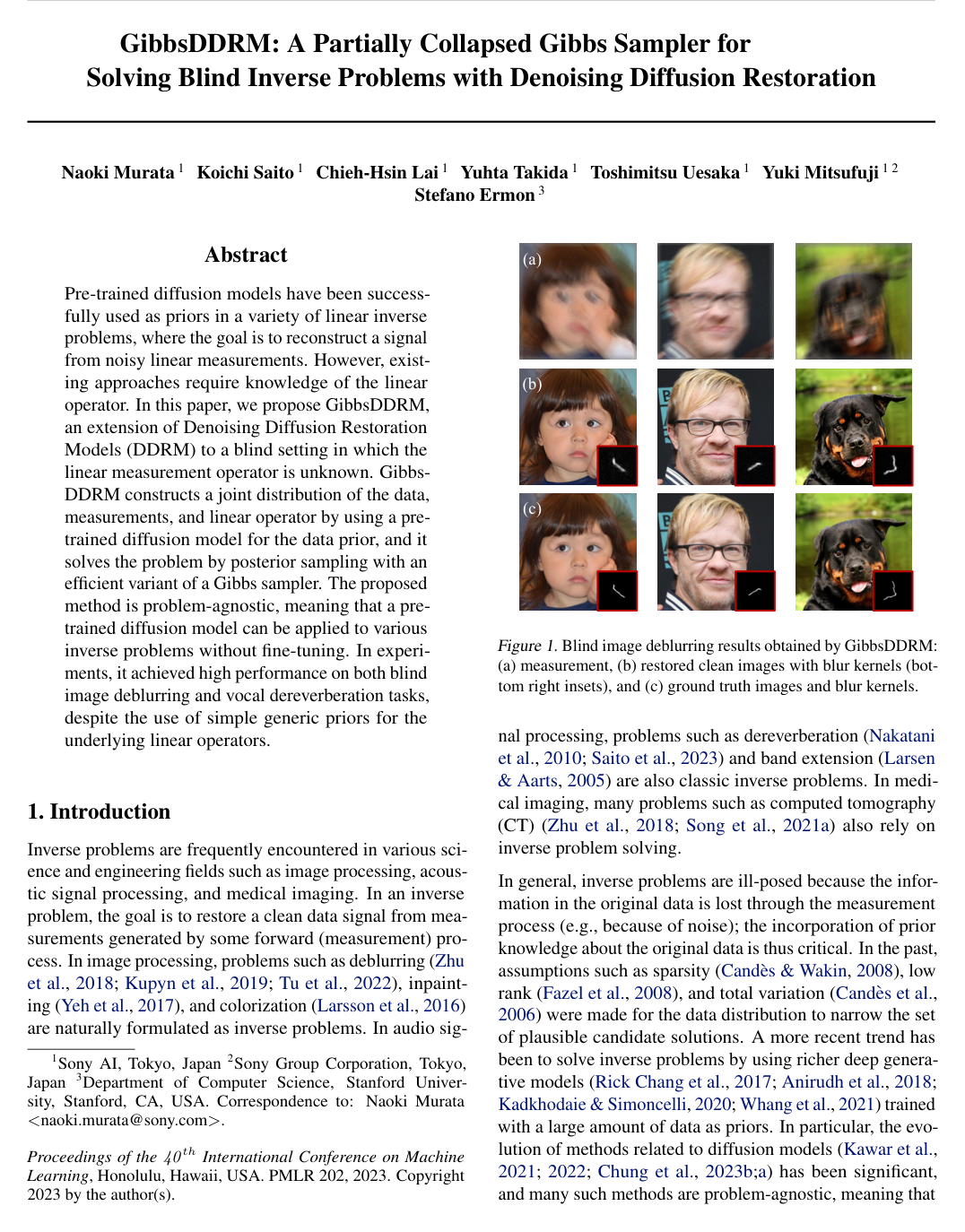
    GibbsDDRM was evaluated on 256×256 motion-blurred images with additive Gaussian measurement noise σy=0.02\sigma_y=0.02, using 1,000 FFHQ validation images and 500 AFHQ dog test images. The blur kernels were 64×64 with intensity 0.5. Pretrained image diffusion models were used without task-specific finetuning. GibbsDDRM used η=0.80\eta=0.80, ηb=0.90\eta_b=0.90, T=100T=100, N=1N=1, and Mt=0M_t=0 for 70≤t≤10070\leq t\leq100 and Mt=3M_t=3 for t<70t<70; operator Langevin sampling used 500 iterations with step size 1.0×10−111.0\times10^{-11}. The kernel was initialized as a normalized Gaussian blur kernel and constrained to remain nonnegative with sum 1; a Laplace prior with diversity parameter λ=103\lambda=10^3 was used.

    The table compares image-distribution quality (FID, lower is better), perceptual fidelity to the ground truth (LPIPS, lower is better), and pixel fidelity (PSNR, higher is better). GibbsDDRM had the best LPIPS among the blind methods on both datasets, whereas MPRNet had higher PSNR. BlindDPS had lower FID than GibbsDDRM but substantially worse LPIPS; its reported result used a pretrained blur-kernel score model, unlike GibbsDDRM's generic operator prior. DDRM with the ground-truth kernel is an oracle, non-blind reference.

    MethodFFHQ FID ↓FFHQ LPIPS ↓FFHQ PSNR ↑AFHQ FID ↓AFHQ LPIPS ↓AFHQ PSNR ↑
    GibbsDDRM38.710.11525.8048.000.19722.01
    MPRNet62.920.21127.2350.430.27827.02
    DeblurGANv2141.550.32019.86156.920.42917.64
    Pan-DCP239.690.65314.20185.400.63214.48
    SelfDeblur283.690.85910.44250.200.84010.34
    BlindDPS*29.490.28122.2423.890.33820.92
    DDRM with ground-truth kernel33.970.06230.6424.600.07829.37

    The paper also reports visually faithful restorations when measurement noise is increased, including the illustrated σy=0.05\sigma_y=0.05 and 0.100.10 cases. Runtime was approximately 56 seconds per image on one RTX3090 with batch size 4.

  7. Knowl 7 — Vocal dereverberation as a blind convolution problem and its evaluation setup

    experimental setup

    For vocal dereverberation, GibbsDDRM models the wet vocal in the short-time Fourier transform (STFT) domain as

    yτ,fwet=∑l=0L−1gl,f∗xτ−l,fdry+zτ,f,y^{\mathrm{wet}}_{\tau,f}=\sum_{l=0}^{L-1}g^*_{l,f}x^{\mathrm{dry}}_{\tau-l,f}+z_{\tau,f},

    where τ\tau and ff index time and frequency, xτ,fdry∈Cx^{\mathrm{dry}}_{\tau,f}\in\mathbb{C} is the unknown dry vocal, gl,f∈Cg_{l,f}\in\mathbb{C} is the unknown acoustic transfer function, LL is reverberation length, zτ,fz_{\tau,f} is additive noise, and ∗* denotes complex conjugation. This is a blind linear convolution operator; its SVD is computed efficiently using an FFT. The diffusion prior is trained on dry vocals from a proprietary dataset totaling approximately 15 hours, and does not require paired wet/dry training for GibbsDDRM.

    Evaluation used 1,000 wet signals totaling about 1.4 hours, created from dry NHSS vocal recordings (100 English pop songs, 285.24 minutes total) with 10 commercial reverb presets having RT60<2RT_{60}<2 seconds. The recordings were monaural at 44.1 kHz; the test signals were assembled as 5-second samples. For diffusion-model input, audio was converted using a 1024-sample Hann STFT window and 256-sample hop, its DC component was removed, and real and imaginary parts were supplied as two channels of 512×512 inputs. The dry-vocal diffusion model had 31.3 million parameters and used 4,000 diffusion steps with a cosine noise schedule.

    Inference used η=0.8\eta=0.8, ηb=0.8\eta_b=0.8, σy=1.0×10⁻³\sigma_y=1.0\times10^{-3}, T=50T=50, N=1N=1, and Mt=0M_t=0 for 40≤t≤5040\leq t\leq50 and Mt=5M_t=5 for t<40t<40. Operator parameters were initialized by one iteration of WPE with L=150L=150 and delay D=4D=4; Langevin sampling used 400 iterations with step size 1.0×10−131.0\times10^{-13} and a Laplace prior with λ=2.0\lambda=2.0.

  8. Knowl 8 — GibbsDDRM outperforms comparison systems on vocal dereverberation metrics

    empirical result

    On the wet-vocal test set, GibbsDDRM was compared with Reverb Conversion (RC), Music Enhancement (ME), and Unsupervised Dereverberation (UD). The evaluation reports Frechet Audio Distance (FAD; lower is better), scale-invariant signal-to-distortion ratio improvement (SI-SDR; higher is better), and speech-to-reverberation modulation energy ratio (SRMR; higher is better). FAD was computed after downsampling signals to 16 kHz. GibbsDDRM achieved the best reported value on all three metrics. In particular, its advantage over UD, which also uses DDRM but estimates the operator differently, is consistent with improved operator estimation. ME performed poorly on SI-SDR; the authors suggest its training/test reverberation mismatch as a possible explanation.

    MethodFAD ↓SI-SDR improvement ↑SRMR ↑
    Wet, unprocessed5.74—7.11
    Reverb Conversion5.690.027.23
    Music Enhancement7.51−23.97.92
    Unsupervised Dereverberation4.990.377.94
    GibbsDDRM4.210.598.40

    GibbsDDRM required about 36 seconds to restore one second of vocal audio, compared with 6 seconds for UD.

  9. Knowl 9 — Langevin sampling stabilizes operator estimation relative to MAP updates

    empirical result

    The paper compared the proposed Langevin updates of the blur-kernel parameters with deterministic maximum-a-posteriori (MAP) updates on 1,000 blind-deblurring images from FFHQ at 256×256 resolution. For this comparison, the MAP update was obtained by removing the Gaussian noise term from the Langevin step, making it a gradient update for the approximate log posterior. Histograms of PSNR and LPIPS showed longer tails for MAP: it could occasionally produce highly accurate restorations, but its outcomes were less stable. The authors interpret the comparison as evidence that Langevin sampling stabilizes estimation of the operator parameters; the paper does not report a numerical aggregate difference for this ablation.

  10. Knowl 10 — Limitation: reliance on a computationally feasible operator SVD

    limitation

    GibbsDDRM relies on an SVD of the current linear measurement operator to perform diffusion restoration in spectral coordinates. The authors identify this as a limitation when the SVD is computationally infeasible, which can make the method difficult to apply to some linear inverse problems. For convolution operators in the image and audio applications, the paper uses FFT-based computation to make the spectral calculations efficient.

Coverage note — No substantial contributed material was omitted; detailed baseline-specific training recipes and supplementary qualitative examples were left out because they do not add distinct core methods or findings beyond the reported evaluations.

References

  1. 1.Anirudh, R., Thiagarajan, J. J., Kailkhura, B., and Bremer, T. An unsupervised approach to solving inverse problems using generative adversarial networks. arXiv preprint arXiv:1805.07281, 2018.
  2. 2.Candes, E. J. and Wakin, M. B. An introduction to compressive sampling. IEEE Signal Process. Mag., 25(2):21–30, 2008.
  3. 3.Candes, E. J., Romberg, J., and Tao, T. Robust uncertainty principles: Exact signal reconstruction from highly incomplete frequency information. IEEE Trans. Inf. Theory, 52(2):489–509, 2006.
  4. 4.Casella, G. and George, E. I. Explaining the Gibbs sampler. The American Statistician, 46(3):167–174, 1992.
  5. 5.Chan, T. F. and Wong, C.-K. Total variation blind deconvolution. IEEE Trans. Image Process., 7(3):370–375, 1998.
  6. 6.Choi, J., Kim, S., Jeong, Y., Gwon, Y., and Yoon, S. ILVR: Conditioning method for denoising diffusion probabilistic models. In Proc. IEEE International Conference on Computer Vision (ICCV), pp. 14347–14356, 2021.
  7. 7.Choi, W., Kim, M., Chung, J., Lee, D., and Jung, S. Investigating U-Nets with various intermediate blocks for spectrogram-based singing voice separation. In Proc. Int. Society for Music Information Retrieval Conf. (ISMIR), 2020a.
  8. 8.Choi, Y., Uh, Y., Yoo, J., and Ha, J.-W. StarGAN v2: Diverse image synthesis for multiple domains. In Proc. IEEE Conference on Computer Vision and Pattern Recognition (CVPR), pp. 8188–8197, 2020b.
  9. 9.Chung, H., Kim, J., Kim, S., and Ye, J. C. Parallel diffusion models of operator and image for blind inverse problems. In Proc. IEEE Conference on Computer Vision and Pattern Recognition (CVPR), 2023a.
  10. 10.Chung, H., Kim, J., Mccann, M. T., Klasky, M. L., and Ye, J. C. Diffusion posterior sampling for general noisy inverse problems. In Proc. International Conference on Learning Representation (ICLR), 2023b.
  11. 11.Dhariwal, P. and Nichol, A. Diffusion models beat GANs on image synthesis. In Proc. Advances in Neural Information Processing Systems (NeurIPS), volume 34, pp. 8780–8794, 2021.
  12. 12.Eaton, J., Gaubitch, N. D., Moore, A. H., and Naylor, P. A. The ace challenge — corpus description and performance evaluation. In 2015 IEEE Workshop on Applications of Signal Processing to Audio and Acoustics (WASPAA), pp. 1–5, 2015. doi: 10.1109/WASPAA.2015.7336912.
  13. 13.Fazel, M., Candes, E., Recht, B., and Parrilo, P. Compressed sensing and robust recovery of low rank matrices. In 2008 42nd Asilomar Conference on Signals, Systems and Computers, pp. 1043–1047. IEEE, 2008.
  14. 14.Gao, X., Sitharam, M., and Roitberg, A. E. Bounds on the Jensen gap, and implications for mean-concentrated distributions. arXiv preprint arXiv:1712.05267, 2017.
  15. 15.Hershey, S., Chaudhuri, S., Ellis, D. P. W., Gemmeke, J. F., Jansen, A., Moore, R. C., Plakal, M., Platt, D., Saurous, R. A., Seybold, B., Slaney, M., Weiss, R. J., and Wilson, K. CNN architectures for large-scale audio classification. In Proc. IEEE Int. Conf. Acoust., Speech, Signal Process. (ICASSP), pp. 131–135, 2017.
  16. 16.Heusel, M., Ramsauer, H., Unterthiner, T., Nessler, B., and Hochreiter, S. GANs trained by a two time-scale update rule converge to a local Nash equilibrium. In Proc. Advances in Neural Information Processing Systems (NeurIPS), pp. 6629–6640, 2017.
  17. 17.Ho, J., Jain, A., and Abbeel, P. Denoising diffusion probabilistic models. Proc. Advances in Neural Information Processing Systems (NeurIPS), 33:6840–6851, 2020.
  18. 18.K. A. Reddy, C., Dubey, H., Koishida, K., Asokan Nair, A., Gopal, V., Cutler, R., Braun, S., Gamper, H., Aichner, R., and Srinivasan, S. Interspeech 2021 deep noise suppression challenge. In Interspeech, 2021.
  19. 19.Kadkhodaie, Z. and Simoncelli, E. P. Solving linear inverse problems using the prior implicit in a denoiser. In NeurIPS 2020 Workshop on Deep Learning and Inverse Problems, 2020.
  20. 20.Kail, G., Tourneret, J.-Y., Hlawatsch, F., and Dobigeon, N. Blind deconvolution of sparse pulse sequences under a minimum distance constraint: A partially collapsed Gibbs sampler method. IEEE Trans. Signal Process., 60(6):2727–2743, 2012.
  21. 21.Kandpal, N., Nieto, O., and Jin, Z. Music enhancement via image translation and vocoding. In Proc. IEEE Int. Conf. Acoust., Speech, Signal Process. (ICASSP), pp. 3124–3128. IEEE, 2022.
  22. 22.Karras, T., Laine, S., and Aila, T. A style-based generator architecture for generative adversarial networks. In Proc. IEEE Conference on Computer Vision and Pattern Recognition (CVPR), pp. 4401–4410, 2019.
  23. 23.Kawar, B., Vaksman, G., and Elad, M. SNIPS: Solving noisy inverse problems stochastically. In Proc. Advances in Neural Information Processing Systems (NeurIPS), volume 34, pp. 21757–21769, 2021.
  24. 24.Kawar, B., Elad, M., Ermon, S., and Song, J. Denoising diffusion restoration models. In Proc. Advances in Neural Information Processing Systems (NeurIPS), 2022.
  25. 25.Kilgour, K., Zuluaga, M., Roblek, D., and Sharifi, M. Frechet Audio Distance: A metric for evaluating music enhancement algorithms. arXiv preprint arXiv:1812.08466, 2018.
  26. 26.Koo, J., Paik, S., and Lee, K. Reverb conversion of mixed vocal tracks using an end-to-end convolutional deep neural network. In Proc. IEEE Int. Conf. Acoust., Speech, Signal Process. (ICASSP), pp. 81–85. IEEE, 2021.
  27. 27.Krishnan, D. and Fergus, R. Fast image deconvolution using hyper-Laplacian priors. In Proc. Advances in Neural Information Processing Systems (NeurIPS), volume 22, 2009.
  28. 28.Kruse, J., Rother, C., and Schmidt, U. Learning to push the limits of efficient FFT-based image deconvolution. In Proc. IEEE International Conference on Computer Vision (ICCV), pp. 4586–4594, 2017.
  29. 29.Kupyn, O., Martyniuk, T., Wu, J., and Wang, Z. Deblurgan-v2: Deblurring (orders-of-magnitude) faster and better. In Proc. IEEE International Conference on Computer Vision (ICCV), pp. 8878–8887, 2019.
  30. 30.Lai, C.-H., Takida, Y., Murata, N., Uesaka, T., Mitsufuji, Y., and Ermon, S. Improving score-based diffusion models by enforcing the underlying score Fokker-Planck equation. 2022.
  31. 31.Langevin, P. On the theory of Brownian motion. 1908.
  32. 32.Larsen, E. and Aarts, R. M. Audio bandwidth extension: application of psychoacoustics, signal processing and loudspeaker design. John Wiley & Sons, 2005.
  33. 33.Larsson, G., Maire, M., and Shakhnarovich, G. Learning representations for automatic colorization. In European conference on computer vision, pp. 577–593. Springer, 2016.
  34. 34.Liu, J. S., Wong, W. H., and Kong, A. Covariance structure of the Gibbs sampler with applications to the comparisons of estimators and augmentation schemes. Biometrika, 81(1):27–40, 1994.
  35. 35.Loshchilov, I. and Hutter, F. Decoupled weight decay regularization. In Proc. International Conference on Learning Representation (ICLR), 2019.
  36. 36.Micikevicius, P., Narang, S., Alben, J., Diamos, G., Elsen, E., Garcia, D., Ginsburg, B., Houston, M., Kuchaiev, O., Venkatesh, G., and Wu, H. Mixed precision training. In Proc. International Conference on Learning Representation (ICLR), 2018.
  37. 37.Miyato, T., Kataoka, T., Koyama, M., and Yoshida, Y. Spectral normalization for generative adversarial networks. In Proc. International Conference on Learning Representation (ICLR), 2018.
  38. 38.Nakatani, T., Yoshioka, T., Kinoshita, K., Miyoshi, M., and Juang, B.-H. Speech dereverberation based on variance-normalized delayed linear prediction. IEEE Trans. Audio, Speech, Lang. Process., 18(7):1717–1731, 2010.
  39. 39.Nichol, A. and Dhariwal, P. Improved denoising diffusion probabilistic models. In Proc. International Conference on Machine Learning (ICML), pp. 8162–8171. PMLR, 2021.
  40. 40.Pan, J., Sun, D., Pfister, H., and Yang, M.-H. Blind image deblurring using dark channel prior. In Proc. IEEE Conference on Computer Vision and Pattern Recognition (CVPR), pp. 1628–1636, 2016.
  41. 41.Pan, J., Sun, D., Pfister, H., and Yang, M.-H. Deblurring images via dark channel prior. IEEE transactions on pattern analysis and machine intelligence, 40(10):2315–2328, 2017.
  42. 42.Parmar, G., Zhang, R., and Zhu, J.-Y. On aliased resizing and surprising subtleties in gan evaluation. In Proc. IEEE Conference on Computer Vision and Pattern Recognition (CVPR), pp. 11410–11420, 2022.
  43. 43.Ren, D., Zhang, K., Wang, Q., Hu, Q., and Zuo, W. Neural blind deconvolution using deep priors. In Proc. IEEE Conference on Computer Vision and Pattern Recognition (CVPR), pp. 3341–3350, 2020.
  44. 44.Rick Chang, J., Li, C.-L., Poczos, B., Vijaya Kumar, B., and Sankaranarayanan, A. C. One network to solve them all–solving linear inverse problems using deep projection models. In Proc. IEEE International Conference on Computer Vision (ICCV), pp. 5888–5897, 2017.
  45. 45.Ronneberger, O., Fischer, P., and Brox, T. U-net: Convolutional networks for biomedical image segmentation. In Proceedings of the International Conference on Medical image computing and computer-assisted intervention, pp. 234–241, 2015.
  46. 46.Roux, J. L., Wisdom, S., Erdogan, H., and Hershey, J. R. SDR – Half-baked or well done? In Proc. IEEE Int. Conf. Acoust., Speech, Signal Process. (ICASSP), pp. 626–630, 2019. doi: 10.1109/ICASSP.2019.8683855.
  47. 47.Saito, K., Murata, N., Uesaka, T., Lai, C.-H., Takida, Y., Fukui, T., and Mitsufuji, Y. Unsupervised vocal dereverberation with diffusion-based generative models. In Proc. IEEE Int. Conf. Acoust., Speech, Signal Process. (ICASSP). IEEE, 2023.
  48. 48.Santos, J. F., Senoussaoui, M., and Falk, T. H. An improved non-intrusive intelligibility metric for noisy and reverberant speech. In Proc. Int. Workshop Acoust. Signal Enhancement (IWAENC), pp. 55–59, 2014. doi: 10.1109/IWAENC.2014.6953337.
  49. 49.Sedghi, H., Gupta, V., and Long, P. M. The singular values of convolutional layers. In Proc. International Conference on Learning Representation (ICLR), 2019.
  50. 50.Sharma, B., Gao, X., Vijayan, K., Tian, X., and Li, H. NHSS: A speech and singing parallel database. Speech Communication, 133:9–22, 2021.
  51. 51.Sohl-Dickstein, J., Weiss, E., Maheswaranathan, N., and Ganguli, S. Deep unsupervised learning using nonequilibrium thermodynamics. In Proc. International Conference on Machine Learning (ICML), pp. 2256–2265. PMLR, 2015.
  52. 52.Song, Y. and Ermon, S. Generative modeling by estimating gradients of the data distribution. Proc. Advances in Neural Information Processing Systems (NeurIPS), 32:11895–11907, 2019.
  53. 53.Song, Y. and Ermon, S. Improved techniques for training score-based generative models. In Proc. Advances in Neural Information Processing Systems (NeurIPS), volume 33, pp. 12438–12448, 2020.
  54. 54.Song, Y., Shen, L., Xing, L., and Ermon, S. Solving inverse problems in medical imaging with score-based generative models. In NeurIPS 2021 Workshop on Deep Learning and Inverse Problems, 2021a.
  55. 55.Song, Y., Sohl-Dickstein, J., Kingma, D. P., Kumar, A., Ermon, S., and Poole, B. Score-based generative modeling through stochastic differential equations. In Proc. International Conference on Learning Representation (ICLR), 2021b.
  56. 56.Tu, Z., Talebi, H., Zhang, H., Yang, F., Milanfar, P., Bovik, A., and Li, Y. MAXIM: Multi-axis MLP for image processing. In Proc. IEEE Conference on Computer Vision and Pattern Recognition (CVPR), pp. 5769–5780, 2022.
  57. 57.Van Dyk, D. A. and Park, T. Partially collapsed Gibbs samplers: Theory and methods. Journal of the American Statistical Association, 103(482):790–796, 2008.
  58. 58.Whang, J., Lei, Q., and Dimakis, A. Solving inverse problems with a flow-based noise model. In Proc. International Conference on Machine Learning (ICML), pp. 11146–11157. PMLR, 2021.
  59. 59.Xu, L., Zheng, S., and Jia, J. Unnatural l0 sparse representation for natural image deblurring. In Proc. IEEE Conference on Computer Vision and Pattern Recognition (CVPR), pp. 1107–1114, 2013.
  60. 60.Yeh, R. A., Chen, C., Yian Lim, T., Schwing, A. G., Hasegawa-Johnson, M., and Do, M. N. Semantic image inpainting with deep generative models. In Proc. IEEE Conference on Computer Vision and Pattern Recognition (CVPR), pp. 5485–5493, 2017.
  61. 61.Zamir, S. W., Arora, A., Khan, S., Hayat, M., Khan, F. S., Yang, M.-H., and Shao, L. Multi-stage progressive image restoration. In Proc. IEEE Conference on Computer Vision and Pattern Recognition (CVPR), pp. 14821–14831, 2021.
  62. 62.Zhang, R., Isola, P., Efros, A. A., Shechtman, E., and Wang, O. The unreasonable effectiveness of deep features as a perceptual metric. In Proc. IEEE Conference on Computer Vision and Pattern Recognition (CVPR), pp. 586–595, 2018.
  63. 63.Zhu, B., Liu, J. Z., Cauley, S. F., Rosen, B. R., and Rosen, M. S. Image reconstruction by domain-transform manifold learning. Nature, 555(7697):487–492, 2018.

Citation

MLA
Murata, N., et al. “GibbsDDRM: A Partially Collapsed Gibbs Sampler for Solving Blind Inverse Problems with Denoising Diffusion Restoration”. International Conference on Machine Learning, vol. 202, 2023, pp. 25501–22, https://proceedings.mlr.press/v202/murata23a.html.
APA
Murata, N., Saito, K., Lai, C.-H., Takida, Y., Uesaka, T., Mitsufuji, Y., & Ermon, S. (2023). GibbsDDRM: A Partially Collapsed Gibbs Sampler for Solving Blind Inverse Problems with Denoising Diffusion Restoration. International Conference on Machine Learning, 202, 25501–25522. https://proceedings.mlr.press/v202/murata23a.html
Chicago
Murata, N., K. Saito, C.-H. Lai, et al. 2023. “GibbsDDRM: A Partially Collapsed Gibbs Sampler for Solving Blind Inverse Problems with Denoising Diffusion Restoration”. International Conference on Machine Learning 202: 25501–22. https://proceedings.mlr.press/v202/murata23a.html.
Harvard
Murata, N. et al. (2023) “GibbsDDRM: A Partially Collapsed Gibbs Sampler for Solving Blind Inverse Problems with Denoising Diffusion Restoration”, International Conference on Machine Learning. PMLR, pp. 25501–25522. Available at: https://proceedings.mlr.press/v202/murata23a.html.
Vancouver
1. Murata N, Saito K, Lai C-H, Takida Y, Uesaka T, Mitsufuji Y, Ermon S (2023) GibbsDDRM: A Partially Collapsed Gibbs Sampler for Solving Blind Inverse Problems with Denoising Diffusion Restoration. In: International Conference on Machine Learning. PMLR, pp 25501–25522

BibTeX

@InProceedings{pmlr-v202-murata23a,
  title = 	 {{G}ibbs{DDRM}: A Partially Collapsed {G}ibbs Sampler for Solving Blind Inverse Problems with Denoising Diffusion Restoration},
  author =       {Murata, Naoki and Saito, Koichi and Lai, Chieh-Hsin and Takida, Yuhta and Uesaka, Toshimitsu and Mitsufuji, Yuki and Ermon, Stefano},
  booktitle = 	 {Proceedings of the 40th International Conference on Machine Learning},
  pages = 	 {25501--25522},
  year = 	 {2023},
  editor = 	 {Krause, Andreas and Brunskill, Emma and Cho, Kyunghyun and Engelhardt, Barbara and Sabato, Sivan and Scarlett, Jonathan},
  volume = 	 {202},
  series = 	 {Proceedings of Machine Learning Research},
  month = 	 {23--29 Jul},
  publisher =    {PMLR},
  pdf = 	 {https://proceedings.mlr.press/v202/murata23a/murata23a.pdf},
  url = 	 {https://proceedings.mlr.press/v202/murata23a.html},
  abstract = 	 {Pre-trained diffusion models have been successfully used as priors in a variety of linear inverse problems, where the goal is to reconstruct a signal from noisy linear measurements. However, existing approaches require knowledge of the linear operator. In this paper, we propose GibbsDDRM, an extension of Denoising Diffusion Restoration Models (DDRM) to a blind setting in which the linear measurement operator is unknown. GibbsDDRM constructs a joint distribution of the data, measurements, and linear operator by using a pre-trained diffusion model for the data prior, and it solves the problem by posterior sampling with an efficient variant of a Gibbs sampler. The proposed method is problem-agnostic, meaning that a pre-trained diffusion model can be applied to various inverse problems without fine-tuning. In experiments, it achieved high performance on both blind image deblurring and vocal dereverberation tasks, despite the use of simple generic priors for the underlying linear operators.}
}
Metadata:DOI registry

Access the Paper

This paper is available from its original source. Click below to access the PDF.

Open PDF
License: https://creativecommons.org/licenses/by/4.0/