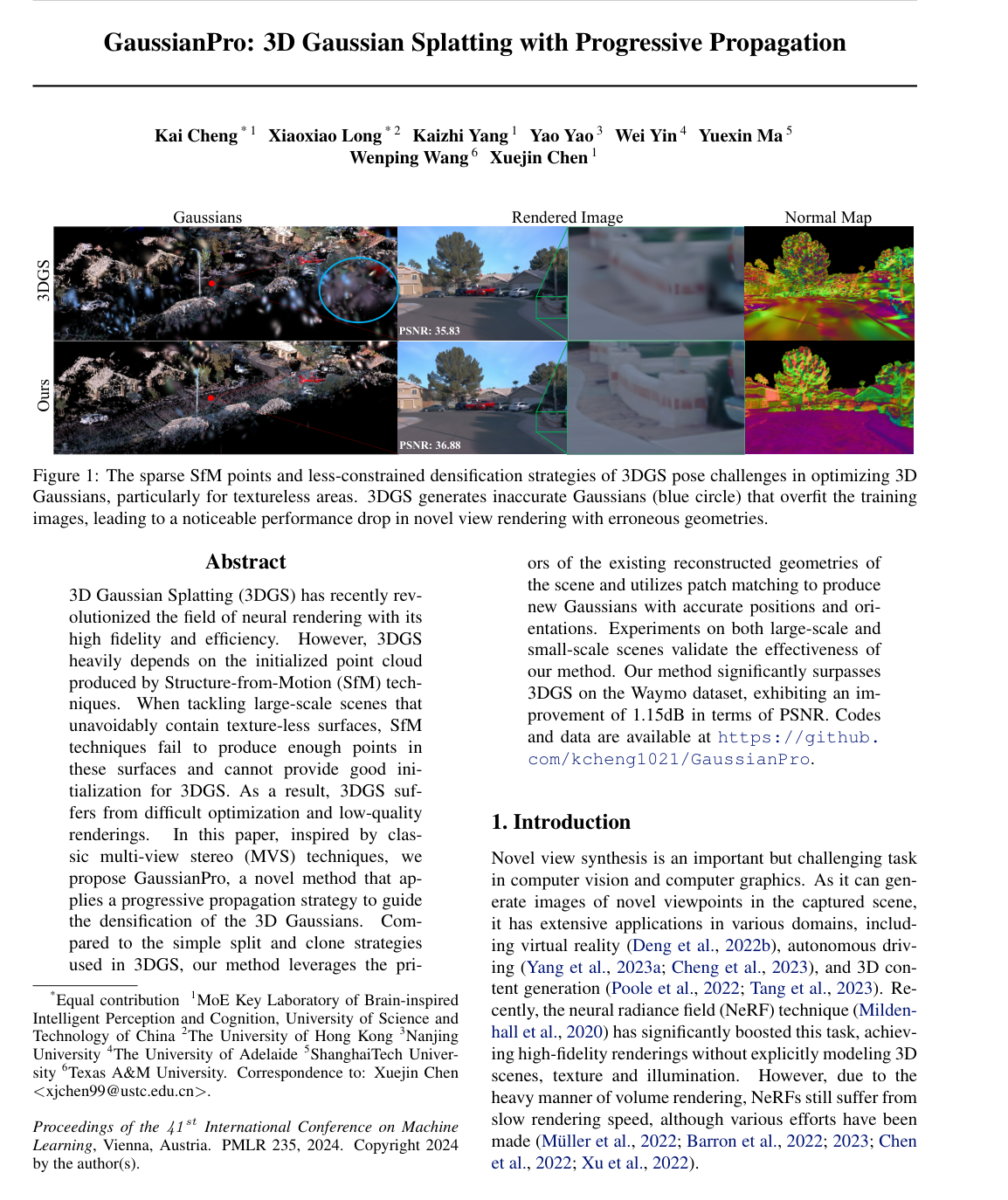
GaussianPro: 3D Gaussian Splatting with Progressive Propagation

Kai ChengXiaoxiao LongKaizhi YangYao YaoWei YinYuexin MaWenping WangXuejin Chen

article2024ICML305 citations

Proposes a multi-view stereo-inspired progressive propagation strategy that guides 3D Gaussian densification via patch matching, resolving initialization failures on texture-less surfaces and improving novel view rendering fidelity across challenging benchmarks.

Listen

Synthesizing novel camera viewpoints from existing imagery is a critical capability for applications in autonomous driving, virtual reality, and 3D digital content creation. The recent 3D Gaussian Splatting technique has significantly accelerated rendering speeds by using 3D Gaussians instead of computationally heavy neural networks. However, the standard method relies heavily on sparse point clouds from initial image matching to populate the scene. In large-scale or textureless environments—such as smooth road surfaces—this approach fails to generate sufficient points, resulting in noisy geometries, missing surfaces, and visual artifacts.

The article develops and evaluates GaussianPro, a new framework that guides the progressive densification and optimization of 3D Gaussians using geometric surface priors. The primary objective is to demonstrate that propagating depth and surface normal information from well-reconstructed areas into under-modeled, low-texture regions improves rendering quality while preserving real-time rendering speeds.

To achieve this, the authors implemented a hybrid approach that bridges 3D space and 2D image projections. The system renders view-dependent depth and normal maps, propagates neighboring geometric values across pixels using patch matching, filters out inconsistent estimates across multiple viewpoints, and back-projects confirmed points into 3D space as new Gaussians. An additional planar loss term is incorporated during training to align Gaussian orientations with local surface planes. The framework was evaluated on the large-scale Waymo autonomous driving dataset and the Mip-NeRF360 benchmark, comparing rendering accuracy, geometric precision, training time, and frame rates against existing methods.

The experimental findings show substantial improvements. First, on the large-scale Waymo dataset, the proposed method significantly outperforms standard 3D Gaussian Splatting, increasing the peak signal-to-noise ratio by 1.15 dB and reducing structural and perceptual image errors. Second, depth reconstruction accuracy improves markedly, reducing the absolute relative depth error from 0.349 to 0.081 and mean absolute error from 6.11 meters to 1.97 meters on Waymo. Third, the system maintains real-time performance, achieving 108 frames per second while adding only a modest increase in training time compared to standard splatting. Finally, the framework demonstrates stronger robustness when trained on reduced numbers of viewpoints and produces a more compact representation with fewer noisy Gaussians than simply lowering densification thresholds.

These results indicate that geometric propagation solves a key failure mode of splatting-based rendering without incurring the severe computational overhead of dense multi-view reconstruction pipelines. For applications requiring both high visual fidelity and real-time performance—such as sensor simulation for autonomous driving—the method provides a practical and scalable solution that avoids the slow rendering bottlenecks of traditional neural radiance fields.

Organizations developing real-time neural rendering or driving simulation pipelines should consider adopting progressive geometric propagation and planar loss constraints into their 3D Gaussian workflows. When dealing with static, structured outdoor and indoor environments, this approach offers a favorable balance of visual fidelity, geometric accuracy, and rendering speed without requiring heavy external reconstruction preprocessing.

The primary limitation identified in the article is that the framework is designed for static environments and does not explicitly model dynamic objects, which can cause artifacts in dynamic scenes. Additionally, rendering gains are modest in small-scale environments with rich textures or intricate high-frequency foliage where initial point coverage is already dense and planar assumptions do not apply. Overall, confidence in the reported improvements for structured and large-scale static scenes is high based on extensive benchmarking.

Cover for GaussianPro: 3D Gaussian Splatting with Progressive Propagation

Abstract

3D Gaussian Splatting (3DGS) has recently revolutionized the field of neural rendering with its high fidelity and efficiency. However, 3DGS heavily depends on the initialized point cloud produced by Structure-from-Motion (SfM) techniques. When tackling large-scale scenes that unavoidably contain texture-less surfaces, SfM techniques fail to produce enough points in these surfaces and cannot provide good initialization for 3DGS. As a result, 3DGS suffers from difficult optimization and low-quality renderings. In this paper, inspired by classic multi-view stereo (MVS) techniques, we propose GaussianPro, a novel method that applies a progressive propagation strategy to guide the densification of the 3D Gaussians. Compared to the simple split and clone strategies used in 3DGS, our method leverages the priors of the existing reconstructed geometries of the scene and utilizes patch matching to produce new Gaussians with accurate positions and orientations. Experiments on both large-scale and small-scale scenes validate the effectiveness of our method. Our method significantly surpasses 3DGS on the Waymo dataset, exhibiting an improvement of 1.15dB in terms of PSNR. Codes and data are available at https://github.com/kcheng1021/GaussianPro.

Table of Contents

  • 1. Introduction
  • 2. Related Work
  • 2.1. Multi-view Stereo
  • 2.2. Neural Radiance Field
  • 2.3. 3D Gaussian Splatting
  • 3. Preliminaries
  • 4. Method
  • 4.1. Hybrid Geometric Representation
  • 4.2. Progressive Gaussian Propagation
  • 4.3. Plane Constraint Optimization
  • 4.4. Training Strategy
  • 5. Experiment
  • 5.1. Datasets and Implementation Details
  • 5.2. Quantative and Qualitative Results
  • 5.3. Ablation Study
  • 6. Conclusion
  • Acknowledgements
  • Impact Statement
  • References
  • A. More Implementation Details of Gaussian Progressive Propagation
  • B. More Ablation Studies
  • C. More Rendering Results
  • D. Results of Each Scene in Waymo and MipNeRF360

Knowls

  1. Knowl 1 — Progressive Gaussian Propagation for 3D Gaussian Densification

    algorithm

    Progressive Gaussian Propagation is a densification mechanism for 3D Gaussian Splatting (3DGS) that transfers geometric information from well-modeled regions to under-modeled or textureless regions using multi-view stereo (MVS) patch matching.

    Input: Current 3D Gaussians {G_i}, training images and camera poses, propagation period m = 50, patch matching iterations u = 3, depth deviation threshold sigma = 0.8
    Output: Updated set of 3D Gaussians with newly densified points
    for each training iteration step = 1 to 30000 do
        Perform standard 3DGS forward rasterization and optimization
        if step mod m == 0 then
            for each active training view do
                Render depth map Z_hat and surface normal map N_hat via alpha-blending
                Convert pixel depths and normals to local 3D planes (d, n)
                for iteration = 1 to u do
                    Collect neighbor plane candidates using a checkerboard pattern
                    Compute homography warps H to neighboring viewpoints
                    Evaluate multi-view photometric consistency with NCC
                    Update pixel plane to the candidate yielding the highest NCC score
                end for
                Derive propagated depth map Z_bar and normal map N_bar
                Apply multi-view geometric consistency check to obtain filtered depth Z_filt and normal N_filt
                Identify pixel set P_new where |Z_filt(p) - Z_hat(p)| / Z_hat(p) > sigma
                Back-project pixels in P_new using Z_filt to generate new 3D points
                Initialize new 3D Gaussians at the generated 3D points and append them to {G_i}
            end for
        end if
    end for
    return {G_i}
  2. Knowl 2 — Hybrid Depth and Surface Normal Rendering for 3D Gaussians

    model/method

    To bridge discrete 3D Gaussians and 2D spatial structures for propagation, 3D Gaussians are projected onto 2D image coordinates to render depth and surface normal maps using differentiable alpha-blending splatting.

    For a viewpoint with camera extrinsic matrix [W,t]∈R3×4[W, t] \in \mathbb{R}^{3 \times 4}, the center μi∈R3×1\mu_i \in \mathbb{R}^{3 \times 1} of a 3D Gaussian GiG_i is transformed into the camera coordinate system: μi′=[xiyizi]=Wμi+t\mu'_i = \begin{bmatrix} x_i \\ y_i \\ z_i \end{bmatrix} = W\mu_i + t where ziz_i is the depth of GiG_i in the current camera frame.

    The covariance matrix Σi∈R3×3\Sigma_i \in \mathbb{R}^{3 \times 3} is decomposed into rotation Ri∈R3×3R_i \in \mathbb{R}^{3 \times 3} and diagonal scale Si=diag⁡(s1,s2,s3)∈R3×3S_i = \operatorname{diag}(s_1, s_2, s_3) \in \mathbb{R}^{3 \times 3} as Σi=RiSiSiTRiT\Sigma_i = R_i S_i S_i^T R_i^T. As Gaussians flatten during optimization, the direction of the shortest axis approximates the surface normal ni∈R3×1n_i \in \mathbb{R}^{3 \times 1}: ni=Ri[r,:],r=argmin⁡([s1,s2,s3])n_i = R_i[r, :], \quad r = \operatorname{argmin}([s_1, s_2, s_3])

    The 2D depth map Z^(p)\hat{Z}(p) and normal map N^(p)\hat{N}(p) at pixel pp are rendered by sorting overlapping Gaussians by ascending depth and computing alpha-blending: Z^(p)=∑i=1Nziαi∏j=1i−1(1−αj),N^(p)=∑i=1Nniαi∏j=1i−1(1−αj)\hat{Z}(p) = \sum_{i=1}^{N} z_i \alpha_i \prod_{j=1}^{i-1} (1 - \alpha_j), \qquad \hat{N}(p) = \sum_{i=1}^{N} n_i \alpha_i \prod_{j=1}^{i-1} (1 - \alpha_j) where αi\alpha_i is the opacity evaluated from the 2D projected Gaussian at pixel pp.

  3. Knowl 3 — Patch-Matching Local Plane Homography and Candidate Selection

    equation

    In progressive Gaussian propagation, each pixel p=(u,v)Tp = (u, v)^T with rendered depth zz and normal nn defines a local 3D tangent plane (d,n)(d, n) where dd is the distance from the camera origin to the plane: d=znTK−1p~d = z n^T K^{-1} \tilde{p} where p~=[u,v,1]T\tilde{p} = [u, v, 1]^T denotes the homogeneous coordinate of pp and K∈R3×3K \in \mathbb{R}^{3 \times 3} is the camera intrinsic matrix.

    Neighboring pixels (selected using a checkerboard pattern) share plane candidates (dkl,nkl)(d_{k_l}, n_{k_l}). A plane candidate induces a planar homography matrix H∈R3×3H \in \mathbb{R}^{3 \times 3} warping homogeneous pixel p~\tilde{p} in the reference view to p~′\tilde{p}' in a neighboring view: p~′≃Hp~\tilde{p}' \simeq H\tilde{p} H=K(Wrel−trelnklTdkl)K−1H = K \left( W_{\text{rel}} - \frac{t_{\text{rel}} n_{k_l}^T}{d_{k_l}} \right) K^{-1} where [Wrel,trel]∈R3×4[W_{\text{rel}}, t_{\text{rel}}] \in \mathbb{R}^{3 \times 4} is the relative rigid transformation between the reference view and the neighboring view.

    The optimal local plane candidate at each pixel is chosen by maximizing the Normalized Cross Correlation (NCC) of patch color consistency across views over u=3u = 3 iterations.

  4. Knowl 4 — Multi-View Geometric Consistency Filtering and Densification Selection

    model/method

    Propagated depth and normal values are filtered through a multi-view geometric consistency check before being used for densification.

    For a reference pixel pp with estimated depth zz, the corresponding depth zgz_g of the warped pixel pgp_g in a nearby target view g∈{1,2,3,4}g \in \{1, 2, 3, 4\} is obtained via: zgp~g=K(WrelK−1zp~+trel)z_g \tilde{p}_g = K (W_{\text{rel}} K^{-1} z \tilde{p} + t_{\text{rel}}) where p~\tilde{p} and p~g\tilde{p}_g are homogeneous coordinates, KK is the camera intrinsic matrix, and [Wrel,trel][W_{\text{rel}}, t_{\text{rel}}] is the relative transformation to target view gg.

    A pixel is retained as geometrically valid (M(p)=1M(p) = 1) if it satisfies depth consistency in at least τ\tau adjacent target views: M(p)={1,if ∑g=14β(∣zg−z∣z)≥τ0,otherwise,β(x)={1,if x<α0,otherwiseM(p) = \begin{cases} 1, & \text{if } \sum_{g=1}^{4} \beta\left( \frac{|z_g - z|}{z} \right) \ge \tau \\ 0, & \text{otherwise} \end{cases}, \quad \beta(x) = \begin{cases} 1, & \text{if } x < \alpha \\ 0, & \text{otherwise} \end{cases}

    From the filtered depth map ZfiltZ_{\text{filt}}, pixels pp exhibiting large discrepancies relative to the currently rendered depth Z^(p)\hat{Z}(p) are identified: ∣Zfilt(p)−Z^(p)∣Z^(p)>σ\frac{|Z_{\text{filt}}(p) - \hat{Z}(p)|}{\hat{Z}(p)} > \sigma where σ=0.8\sigma = 0.8. Such pixels indicate regions under-modeled by existing Gaussians. They are back-projected to 3D coordinates using Zfilt(p)Z_{\text{filt}}(p) and initialized as new 3D Gaussians for subsequent optimization.

  5. Knowl 5 — Planar Constraint Optimization Loss

    equation

    To prevent 3D Gaussians from deviating into noisy, non-physical geometry in low-texture planar areas, GaussianPro incorporates a planar constraint loss LplanarL_{\text{planar}} during optimization.

    The normal supervision loss LnormalL_{\text{normal}} minimizes the L1L_1 and angular deviation between the rendered normal map N^\hat{N} and the propagated, geometrically filtered normal map Nˉ\bar{N} over the valid pixel set QQ: Lnormal=∑p∈Q(∥N^(p)−Nˉ(p)∥1+∣1−N^(p)TNˉ(p)∣1)L_{\text{normal}} = \sum_{p \in Q} \left( \|\hat{N}(p) - \bar{N}(p)\|_1 + \left| 1 - \hat{N}(p)^T \bar{N}(p) \right|_1 \right)

    The total planar constraint combines normal supervision with Gaussian scale regularization LscaleL_{\text{scale}} (which forces the smallest Gaussian axis length towards zero to flatten Gaussians onto surfaces): Lplanar=βLnormal+γLscaleL_{\text{planar}} = \beta L_{\text{normal}} + \gamma L_{\text{scale}} where hyperparameters are set to β=0.001\beta = 0.001 and γ=100\gamma = 100.

    The overall optimization objective is: L=(1−λ)L1+λLD-SSIM+LplanarL = (1 - \lambda) L_1 + \lambda L_{\text{D-SSIM}} + L_{\text{planar}} where λ=0.2\lambda = 0.2, L1L_1 is the photometric absolute error, and LD-SSIML_{\text{D-SSIM}} is the structural dissimilarity loss.

  6. Knowl 6 — Quantitative Evaluation on Waymo and Mip-NeRF360 Benchmarks

    data/table

    GaussianPro was evaluated on the large-scale autonomous driving dataset Waymo (9 scenes, 1 out of every 8 images held out for testing) and the Mip-NeRF360 dataset. Comparison models include Instant-NGP, Mip-NeRF 360, Zip-NeRF, and baseline 3DGS.

    Waymo MipNeRF 360
    Method FPS ↑\uparrow PSNR ↑\uparrow SSIM ↑\uparrow LPIPS ↓\downarrow PSNR ↑\uparrow SSIM ↑\uparrow LPIPS ↓\downarrow
    Instant-NGP 3 30.98 0.886 0.281 25.59 0.699 0.331
    Mip-NeRF 360 0.02 30.09 0.909 0.262 27.69 0.792 0.237
    Zip-NeRF 0.09 34.22 0.939 0.205 28.54 0.828 0.189
    3DGS 103 33.53 0.938 0.226 27.21 0.815 0.214
    3DGS (Retrained) 102 - - - 27.88 0.824 0.209
    GaussianPro (Ours) 108 34.68 0.949 0.191 27.92 0.825 0.208

    On Waymo, GaussianPro achieves an improvement of 1.15 dB PSNR over baseline 3DGS while maintaining real-time rendering speeds (108 FPS), outperforming NeRF-based methods on all metrics. On Mip-NeRF360, GaussianPro outperforms 3DGS on weak-texture and indoor scenes while maintaining comparable performance on dense-texture outdoor scenes.

  7. Knowl 7 — Ablation Study on Progressive Propagation and Planar Constraints

    data/table

    An ablation study conducted on the Waymo dataset evaluates the individual and joint contributions of the progressive propagation densification strategy and the planar constraint loss.

    Propagation Planar PSNR ↑\uparrow SSIM ↑\uparrow LPIPS ↓\downarrow
    ×\times ×\times 33.53 0.938 0.226
    ×\times ✓ 34.02 0.942 0.218
    ✓ ×\times 34.48 0.946 0.203
    ✓ ✓ 34.68 0.949 0.191

    Adding progressive propagation yields a +0.95 dB PSNR gain over baseline 3DGS, and adding planar regularizations adds another +0.20 dB (for a total gain of +1.15 dB PSNR), showing that both accurate Gaussian geometric placement and surface normal alignment contribute to the rendering quality improvements.

  8. Knowl 8 — Reconstruction Quality versus Gaussian Count and Compactness

    empirical result

    In 3D Gaussian Splatting, increasing the number of Gaussians via densification can improve fitting capacity, but without geometric constraints it produces redundant or noisy Gaussians.

    On Waymo:

    • Baseline 3DGS generates 992k Gaussians and achieves 33.53 dB PSNR.
    • 3DGS with a lower gradient densification threshold (3DGS*) produces 1629k Gaussians and achieves 33.89 dB PSNR.
    • GaussianPro produces 1147k Gaussians and achieves 34.68 dB PSNR.

    On Mip-NeRF360:

    • Baseline 3DGS utilizes 3362k Gaussians (27.21 dB PSNR).
    • Retrained 3DGS with improved SfM points utilizes 3009k Gaussians (27.88 dB PSNR).
    • GaussianPro utilizes 2773k Gaussians (27.92 dB PSNR).

    GaussianPro outperforms 3DGS variants even when 3DGS uses substantially more Gaussians (e.g., 1629k vs 1147k), demonstrating that the performance gain is driven by accurate geometric placement and orientation rather than Gaussian quantity.

  9. Knowl 9 — Quantitative Evaluation of Rendered Geometry Accuracy

    data/table

    The geometric accuracy of scene reconstruction was evaluated on the Waymo dataset by comparing the depth maps rendered from the optimized 3D Gaussians against ground-truth depths using Absolute Relative error (Abs Rel), Mean Absolute Error (MAE in meters), and threshold accuracy δ1\delta_1 (fraction of pixels with max⁡(z/z∗,z∗/z)<1.25\max(z/z^*, z^*/z) < 1.25).

    Method Abs Rel ↓\downarrow MAE(m) ↓\downarrow δ1↑\delta_1 \uparrow
    3DGS 0.349 6.11 0.570
    GaussianPro 0.081 1.97 0.933

    GaussianPro decreases absolute relative depth error from 0.349 to 0.081 and mean absolute error from 6.11 m to 1.97 m, while improving δ1\delta_1 accuracy from 57.0% to 93.3%.

  10. Knowl 10 — Efficiency and Novel-View Robustness under Sparse Views

    empirical result

    GaussianPro exhibits stability under sparse view training and computational efficiency compared to dense MVS point initialization:

    1. Sparse View Robustness: When training on random view subsets (30%, 50%, 70%, 100%) of the Mip-NeRF360 room scene:

      • 30% views: 3DGS achieves 28.45 dB PSNR / 0.896 SSIM / 0.216 LPIPS; GaussianPro achieves 28.64 dB PSNR / 0.900 SSIM / 0.210 LPIPS.
      • 50% views: 3DGS achieves 29.97 dB / 0.912 / 0.203; GaussianPro achieves 30.27 dB / 0.914 / 0.199.
      • 70% views: 3DGS achieves 30.87 dB / 0.921 / 0.194; GaussianPro achieves 30.93 dB / 0.924 / 0.189.
      • 100% views: 3DGS achieves 31.71 dB / 0.919 / 0.192; GaussianPro achieves 31.98 dB / 0.927 / 0.192.
    2. Efficiency relative to MVS: Directly initializing 3DGS with dense MVS point clouds requires approximately 4×4\times total training time (250–270 minutes vs 56–70 minutes for GaussianPro) due to dense point initialization and slow MVS reconstruction, producing 1.7M–1.8M Gaussians and reduced rendering framerates (75–90 FPS vs 108–113 FPS for GaussianPro).

  11. Knowl 11 — Limitation: Modeling of Dynamic Moving Objects in Static Scenes

    limitation

    GaussianPro assumes static scene geometry and planar surface priors. In outdoor autonomous driving scenarios containing moving objects (e.g., dynamic vehicles or pedestrians), the static Gaussian representation cannot capture temporal motion, resulting in motion blur or geometric artifacts in dynamic regions unless combined with explicit dynamic or deformable Gaussian extensions.

Coverage note — None was omitted; all key contributions including progressive Gaussian propagation, normal derivation and hybrid rendering, homography plane formulation, geometric filtering, planar losses, ablation studies, and quantitative benchmarks are covered.

References

  1. 1.Barron, J. T., Mildenhall, B., Tancik, M., Hedman, P., Martin-Brualla, R., and Srinivasan, P. P. Mip-Nerf: A multiscale representation for anti-aliasing neural radiance fields. In Proceedings of the IEEE/CVF International Conference on Computer Vision, pp. 5855–5864, 2021.
  2. 2.Barron, J. T., Mildenhall, B., Verbin, D., Srinivasan, P. P., and Hedman, P. Mip-Nerf 360: Unbounded anti-aliased neural radiance fields. In Proceedings of the IEEE/CVF Conference on Computer Vision and Pattern Recognition, pp. 5470–5479, 2022.
  3. 3.Barron, J. T., Mildenhall, B., Verbin, D., Srinivasan, P. P., and Hedman, P. Zip-Nerf: Anti-aliased grid-based neural radiance fields. Proceedings of the IEEE International Conference on Computer Vision, 2023.
  4. 4.Bleyer, M., Rhemann, C., and Rother, C. Patchmatch stereo-stereo matching with slanted support windows. In BMVC, volume 11, pp. 1–11, 2011.
  5. 5.Caesar, H., Bankiti, V., Lang, A. H., Vora, S., Liong, V. E., Xu, Q., Krishnan, A., Pan, Y., Baldan, G., and Beijbom, O. NuScenes: A multimodal dataset for autonomous driving. In Proceedings of the IEEE/CVF conference on computer vision and pattern recognition, pp. 11621–11631, 2020.
  6. 6.Campbell, N. D., Vogiatzis, G., Hernández, C., and Cipolla, R. Using multiple hypotheses to improve depthmaps for multi-view stereo. In 10th European Conference on Computer Vision, Marseille, France, October 12-18, 2008, Proceedings, Part I 10, pp. 766–779. Springer, 2008.
  7. 7.Chen, A., Xu, Z., Geiger, A., Yu, J., and Su, H. Tensorf: Tensorial radiance fields. In European Conference on Computer Vision, pp. 333–350. Springer, 2022.
  8. 8.Chen, H., Li, C., and Lee, G. H. NeuSG: Neural implicit surface reconstruction with 3D gaussian splatting guidance. arXiv preprint arXiv:2312.00846, 2023.
  9. 9.Chen, R., Han, S., Xu, J., and Su, H. Point-based multiview stereo network. In Proceedings of the IEEE/CVF international conference on computer vision, pp. 1538–1547, 2019.
  10. 10.Cheng, K., Long, X., Yin, W., Wang, J., Wu, Z., Ma, Y., Wang, K., Chen, X., and Chen, X. UC-Nerf: Neural radiance field for under-calibrated multi-view cameras. In The Twelfth International Conference on Learning Representations, 2023.
  11. 11.Deng, K., Liu, A., Zhu, J.-Y., and Ramanan, D. Depthsupervised Nerf: Fewer views and faster training for free. In Proceedings of the IEEE/CVF Conference on Computer Vision and Pattern Recognition, pp. 12882–12891, 2022a.
  12. 12.Deng, N., He, Z., Ye, J., Duinkharjav, B., Chakravarthula, P., Yang, X., and Sun, Q. Fov-Nerf: Foveated neural radiance fields for virtual reality. IEEE Transactions on Visualization and Computer Graphics, 28(11):3854–3864, 2022b.
  13. 13.Fan, Z., Wang, K., Wen, K., Zhu, Z., Xu, D., and Wang, Z. LightGaussian: Unbounded 3D Gaussian compression with 15x reduction and 200+ fps. arXiv preprint arXiv:2311.17245, 2023.
  14. 14.Feng, Z., Yang, L., Guo, P., and Li, B. CVRecon: Rethinking 3D geometric feature learning for neural reconstruction. In Proceedings of the IEEE/CVF International Conference on Computer Vision, pp. 17750–17760, 2023.
  15. 15.Fridovich-Keil, S., Yu, A., Tancik, M., Chen, Q., Recht, B., and Kanazawa, A. Plenoxels: Radiance fields without neural networks. In Proceedings of the IEEE/CVF Conference on Computer Vision and Pattern Recognition, pp. 5501–5510, 2022.
  16. 16.Furukawa, Y. and Ponce, J. Accurate, dense, and robust multiview stereopsis. IEEE transactions on pattern analysis and machine intelligence, 32(8):1362–1376, 2009.
  17. 17.Furukawa, Y., Hernández, C., et al. Multi-view stereo: A tutorial. Foundations and Trends® in Computer Graphics and Vision, 9(1-2):1–148, 2015.
  18. 18.Jiang, Y., Tu, J., Liu, Y., Gao, X., Long, X., Wang, W., and Ma, Y. GaussianShader: 3D gaussian splatting with shading functions for reflective surfaces. arXiv preprint arXiv:2311.17977, 2023.
  19. 19.Kerbl, B., Kopanas, G., Leimkóhler, T., and Drettakis, G. 3D Gaussian splatting for real-time radiance field rendering. ACM Transactions on Graphics, 42(4), 2023.
  20. 20.Laina, I., Rupprecht, C., Belagiannis, V., Tombari, F., and Navab, N. Deeper depth prediction with fully convolutional residual networks. In 2016 Fourth international conference on 3D vision (3DV), pp. 239–248. IEEE, 2016.
  21. 21.Lee, J. C., Rho, D., Sun, X., Ko, J. H., and Park, E. Compact 3D Gaussian representation for radiance field. arXiv preprint arXiv:2311.13681, 2023.
  22. 22.Li, Z., Chen, Z., Li, Z., and Xu, Y. Spacetime gaussian feature splatting for real-time dynamic view synthesis. arXiv preprint arXiv:2312.16812, 2023.
  23. 23.Lin, Y., Dai, Z., Zhu, S., and Yao, Y. Gaussian-flow: 4D reconstruction with dynamic 3D gaussian particle. arXiv preprint arXiv:2312.03431, 2023.
  24. 24.Liu, L., Gu, J., Zaw Lin, K., Chua, T.-S., and Theobalt, C. Neural sparse voxel fields. Advances in Neural Information Processing Systems, 33:15651–15663, 2020.
  25. 25.Long, X., Liu, L., Theobalt, C., and Wang, W. Occlusion-aware depth estimation with adaptive normal constraints. In Computer Vision–ECCV 2020: 16th European Conference, Glasgow, UK, August 23–28, 2020, Proceedings, Part IX 16, pp. 640–657. Springer, 2020.
  26. 26.Long, X., Liu, L., Li, W., Theobalt, C., and Wang, W. Multi-view depth estimation using epipolar spatio-temporal networks. In Proceedings of the IEEE/CVF Conference on Computer Vision and Pattern Recognition, pp. 8258–8267, 2021.
  27. 27.Long, X., Lin, C., Wang, P., Komura, T., and Wang, W. SparseNeus: Fast generalizable neural surface reconstruction from sparse views. In European Conference on Computer Vision, pp. 210–227. Springer, 2022.
  28. 28.Lu, T., Yu, M., Xu, L., Xiangli, Y., Wang, L., Lin, D., and Dai, B. Scaffold-GS: Structured 3D Gaussians for view-adaptive rendering. arXiv preprint arXiv:2312.00109, 2023.
  29. 29.Ma, Z., Teed, Z., and Deng, J. Multiview stereo with cascaded epipolar RAFT. In European Conference on Computer Vision, pp. 734–750. Springer, 2022.
  30. 30.Mildenhall, B., Srinivasan, P., Tancik, M., Barron, J., Ramamoorthi, R., and Ng, R. Nerf: Representing scenes as neural radiance fields for view synthesis. In European conference on computer vision, 2020.
  31. 31.Morgenstern, W., Barthel, F., Hilsmann, A., and Eisert, P. Compact 3D scene representation via self-organizing gaussian grids. arXiv preprint arXiv:2312.13299, 2023.
  32. 32.Müller, T., Evans, A., Schied, C., and Keller, A. Instant neural graphics primitives with a multiresolution hash encoding. ACM Transactions on Graphics (ToG), 41(4): 1–15, 2022.
  33. 33.Murez, Z., Van As, T., Bartolozzi, J., Sinha, A., Badrinarayanan, V., and Rabinovich, A. Atlas: End-to-end 3d scene reconstruction from posed images. In Computer Vision–ECCV 2020: 16th European Conference, Glasgow, UK, August 23–28, 2020, Proceedings, Part VII 16, pp. 414–431. Springer, 2020.
  34. 34.Navaneet, K., Meibodi, K. P., Koohpayegani, S. A., and Pirsiavash, H. Compact3D: Compressing Gaussian splat radiance field models with vector quantization. arXiv preprint arXiv:2311.18159, 2023.
  35. 35.Poole, B., Jain, A., Barron, J. T., and Mildenhall, B. DreamFusion: Text-to-3D using 2D diffusion. In The Eleventh International Conference on Learning Representations, 2022.
  36. 36.Schönberger, J. L., Zheng, E., Frahm, J.-M., and Pollefeys, M. Pixelwise view selection for unstructured multi-view stereo. In Computer Vision–ECCV 2016: 14th European Conference, Amsterdam, The Netherlands, October 11-14, 2016, Proceedings, Part III 14, pp. 501–518. Springer, 2016.
  37. 37.Sun, P., Kretzschmar, H., Dotiwalla, X., Chouard, A., Patnaik, V., Tsui, P., Guo, J., Zhou, Y., Chai, Y., Caine, B., et al. Scalability in perception for autonomous driving: Waymo open dataset. In Proceedings of the IEEE/CVF conference on computer vision and pattern recognition, pp. 2446–2454, 2020.
  38. 38.Tang, J., Ren, J., Zhou, H., Liu, Z., and Zeng, G. Dreamgaussian: Generative gaussian splatting for efficient 3D content creation. arXiv preprint arXiv:2309.16653, 2023.
  39. 39.Wang, P., Liu, Y., Chen, Z., Liu, L., Liu, Z., Komura, T., Theobalt, C., and Wang, W. F2-Nerf: Fast neural radiance field training with free camera trajectories. In Proceedings of the IEEE/CVF Conference on Computer Vision and Pattern Recognition, pp. 4150–4159, 2023.
  40. 40.Xie, E., Wang, W., Yu, Z., Anandkumar, A., Alvarez, J. M., and Luo, P. SegFormer: Simple and efficient design for semantic segmentation with transformers. Advances in neural information processing systems, 34: 12077–12090, 2021.
  41. 41.Xu, Q. and Tao, W. Multi-scale geometric consistency guided multi-view stereo. In Proceedings of the IEEE/CVF Conference on Computer Vision and Pattern Recognition, pp. 5483–5492, 2019.
  42. 42.Xu, Q., Xu, Z., Philip, J., Bi, S., Shu, Z., Sunkavalli, K., and Neumann, U. Point-Nerf: Point-based neural radiance fields. In Proceedings of the IEEE/CVF Conference on Computer Vision and Pattern Recognition, pp. 5438–5448, 2022.
  43. 43.Yan, Y., Lin, H., Zhou, C., Wang, W., Sun, H., Zhan, K., Lang, X., Zhou, X., and Peng, S. Street gaussians for modeling dynamic urban scenes. arXiv preprint arXiv:2401.01339, 2024.
  44. 44.Yan, Z., Low, W. F., Chen, Y., and Lee, G. H. Multi-scale 3D Gaussian splatting for anti-aliased rendering. arXiv preprint arXiv:2311.17089, 2023.
  45. 45.Yang, Z., Chen, Y., Wang, J., Manivasagam, S., Ma, W.-C., Yang, A. J., and Urtasun, R. UniSim: A neural closed-loop sensor simulator. In Proceedings of the IEEE/CVF Conference on Computer Vision and Pattern Recognition, pp. 1389–1399, 2023a.
  46. 46.Yang, Z., Gao, X., Zhou, W., Jiao, S., Zhang, Y., and Jin, X. Deformable 3D Gaussians for high-fidelity monocular dynamic scene reconstruction. arXiv preprint arXiv:2309.13101, 2023b.
  47. 47.Yao, Y., Luo, Z., Li, S., Fang, T., and Quan, L. Mvsnet: Depth inference for unstructured multi-view stereo. In Proceedings of the European conference on computer vision (ECCV), pp. 767–783, 2018.
  48. 48.Yifan, W., Serena, F., Wu, S., Öztireli, C., and Sorkine-Hornung, O. Differentiable surface splatting for point-based geometry processing. ACM Transactions on Graphics (TOG), 38(6):1–14, 2019.
  49. 49.Yoo, J.-C. and Han, T. H. Fast normalized cross-correlation. Circuits, systems and signal processing, 28: 819–843, 2009.
  50. 50.Yu, Z., Peng, S., Niemeyer, M., Sattler, T., and Geiger, A. Monosdf: Exploring monocular geometric cues for neural implicit surface reconstruction. Advances in neural information processing systems, 35:25018–25032, 2022.
  51. 51.Yu, Z., Chen, A., Huang, B., Sattler, T., and Geiger, A. Mip-Splatting: Alias-free 3D gaussian splatting. arXiv preprint arXiv:2311.16493, 2023.
  52. 52.Zhang, R., Isola, P., Efros, A. A., Shechtman, E., and Wang, O. The unreasonable effectiveness of deep features as a perceptual metric. In Proceedings of the IEEE conference on computer vision and pattern recognition, pp. 586–595, 2018.
  53. 53.Zhou, X., Lin, Z., Shan, X., Wang, Y., Sun, D., and Yang, M.-H. DrivingGaussian: Composite gaussian splatting for surrounding dynamic autonomous driving scenes. arXiv preprint arXiv:2312.07920, 2023.
  54. 54.Zwicker, M., Pfister, H., Van Baar, J., and Gross, M. EWA splatting. IEEE Transactions on Visualization and Computer Graphics, 8(3):223–238, 2002.

Citation

MLA
Cheng, K., et al. “GaussianPro: 3D Gaussian Splatting with Progressive Propagation”. arXiv, 2024, http://arxiv.org/abs/2402.14650v1.
APA
Cheng, K., Long, X., Yang, K., Yao, Y., Yin, W., Ma, Y., Wang, W., & Chen, X. (2024). GaussianPro: 3D Gaussian Splatting with Progressive Propagation. arXiv. http://arxiv.org/abs/2402.14650v1
Chicago
Cheng, K., X. Long, K. Yang, et al. 2024. “GaussianPro: 3D Gaussian Splatting with Progressive Propagation”. arXiv. http://arxiv.org/abs/2402.14650v1.
Harvard
Cheng, K. et al. (2024) “GaussianPro: 3D Gaussian Splatting with Progressive Propagation”, arXiv [Preprint]. Available at: http://arxiv.org/abs/2402.14650v1.
Vancouver
1. Cheng K, Long X, Yang K, Yao Y, Yin W, Ma Y, Wang W, Chen X (2024) GaussianPro: 3D Gaussian Splatting with Progressive Propagation. arXiv

BibTeX

@article{cheng2024gaussianpro,
  title = {GaussianPro: 3D Gaussian Splatting with Progressive Propagation},
  author = {Cheng, Kai and Long, Xiaoxiao and Yang, Kaizhi and Yao, Yao and Yin, Wei and Ma, Yuexin and Wang, Wenping and Chen, Xuejin},
  year = {2024},
  journal = {arXiv},
  url = {http://arxiv.org/abs/2402.14650v1},
  eprint = {2402.14650}
}
Metadata:arXiv

Source Code

This paper has an official code repository available. Click below to access the source code.

View Repository

Access the Paper

This paper is available from its original source. Click below to access the PDF.

Open PDF
License: https://creativecommons.org/licenses/by/4.0/