Pixelwise View Selection for Unstructured Multi-View Stereo

Johannes L. SchönbergerEnliang ZhengJan-Michael FrahmM. Pollefeys

article2016ECCV2,922 citations

Presents the dense reconstruction pipeline behind COLMAP, which jointly estimates depth and surface normals using PatchMatch and selects optimal source views at the pixel level through photometric and geometric priors.

Listen

This paper introduces an improved multi-view stereo method that produces accurate, complete three-dimensional scene models from large, unstructured collections of photographs taken under uncontrolled conditions. The work addresses the persistent difficulty of recovering reliable dense geometry when input images vary widely in resolution, illumination, viewpoint, and registration quality, a setting common to crowd-sourced Internet photo collections that now underpin many mapping and visualization applications.

The authors set out to demonstrate that embedding per-pixel surface normals, geometric view-selection priors, bilateral photometric weighting, temporal smoothness on visibility, and a multi-view geometric consistency term inside an existing variational inference framework can simultaneously raise accuracy, completeness, and efficiency over prior art.

They evaluated the approach on standard benchmarks (Middlebury and Strecha) that supply ground-truth geometry and on a world-scale Internet photo collection of roughly 100 million images. Experiments compared full and ablated versions of the algorithm, measured runtime on GPU hardware, and assessed both raw depth maps and the final fused point clouds.

The method ranked first or tied for first on several Middlebury test cases and produced the highest accuracy and completeness scores on the Strecha Fountain and Herzjesu sequences. On the large Internet dataset it generated visually coherent reconstructions of major landmarks while running in roughly four days on a modest multi-GPU workstation. Each added component—normal estimation, geometric priors, temporal smoothness, bilateral weighting, and geometric consistency—measurably improved both completeness and outlier rejection, with the combined system yielding essentially outlier-free depth and normal maps that can be fused directly or meshed without further cleaning.

These gains matter because they remove the need for restrictive pre-selection of image clusters or heavy post-processing, thereby making high-quality dense modeling practical for the noisy, heterogeneous data that dominate real-world capture campaigns. The resulting point clouds support immediate meshing, texturing, and downstream tasks such as localization or rendering.

The authors have released the full implementation as part of the open-source COLMAP package, enabling immediate adoption and further experimentation. Additional gains are likely from tighter integration with semantic cues or dynamic scene handling, but the current evidence already shows that the proposed formulation is ready for production use on large unstructured collections. The principal remaining uncertainties concern performance on extremely low-texture or rapidly changing scenes, where the photometric and geometric assumptions may still break down.

ETH Zurich Microsoft University of North Carolina at Chapel Hill genetic selection multi-view stereo view selection Multi‑View Stereo Pixelwise View Selection Depth Normal Estimation

colmap/colmap Schönberger et al (2016).pdf

Paper: A Comparison and Evaluation of Multi-View Stereo Reconstruction Algorithms, S. Seitz et al. (2006). Reading this foundational multi-view stereo evaluation benchmark and taxonomy provides essential background on the performance metrics and algorithmic challenges that the source paper directly addresses.
Paper: A volumetric method for building complex models from range images, B. Curless et al. (1996). Understanding this volumetric range-image integration method is crucial, as the source paper builds upon its principles of signed distance fields and surface fusion for depth and normal refinement.

Paper: NeuS: Learning Neural Implicit Surfaces by Volume Rendering for Multi-view Reconstruction, Peng Wang et al. (2021). This work extends traditional multi-view stereo and reconstruction pipelines by demonstrating how neural implicit surfaces can be learned via volume rendering without requiring explicit depth maps.
Paper: 3D Gaussian Splatting for Real-Time Radiance Field Rendering, Bernhard Kerbl et al. (2023). This paper builds directly on multi-view stereo and radiance field concepts to introduce a real-time rendering approach using 3D Gaussian primitives instead of slow volumetric ray marching.

Cover for Pixelwise View Selection for Unstructured Multi-View Stereo

Abstract

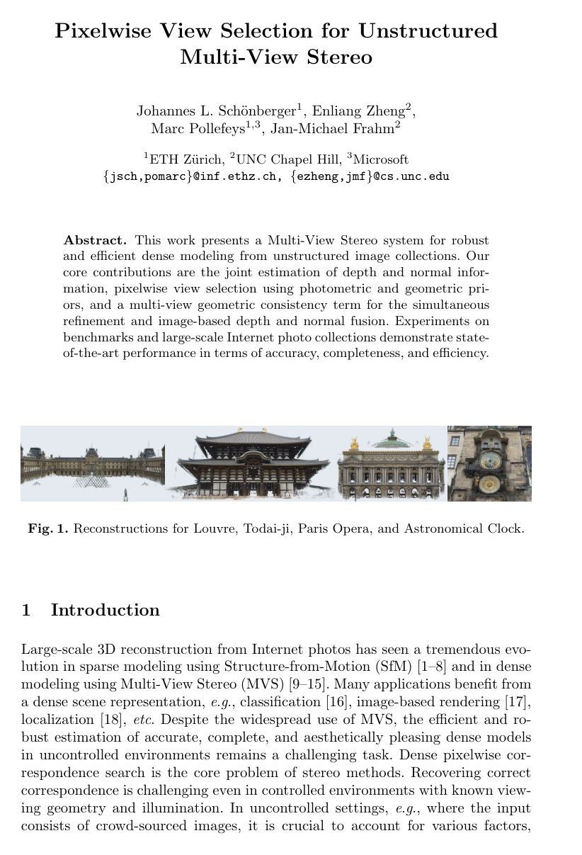
This work presents a Multi-View Stereo system for robust and efficient dense modeling from unstructured image collections. Our core contributions are the joint estimation of depth and normal information, pixelwise view selection using photometric and geometric priors, and a multi-view geometric consistency term for the simultaneous refinement and image-based depth and normal fusion. Experiments on benchmarks and large-scale Internet photo collections demonstrate state-of-the-art performance in terms of accuracy, completeness, and efficiency.

Topics

genetic selection multi-view stereo view selection viewpoint

Keywords

Multi‑View Stereo Pixelwise View Selection Depth Normal Estimation Geometric Prior Photometric Consistency Temporal Smoothness PatchMatch Sampling Sparse Reconstruction Large‑Scale Internet Photo Benchmark Result

1 Introduction
2 Related Work
3 Review of Joint View Selection and Depth Estimation
4 Algorithm
4.1 Normal Estimation
4.2 Geometric Priors for View Selection
4.3 View Selection Smoothness
4.4 Photometric Consistency
4.5 Geometric Consistency
4.6 Integration
4.7 Filtering and Fusion
5 Experiments
6 Conclusion
References

Knowls

Knowl 1 — Joint Depth and Normal Estimation using Slanted-Plane Homography Warping
model/method
In multi-view stereo, mapping image patches between a reference view and source views using slanted planes avoids matching distortions for oblique surface structures. Let $x_l \in \mathbb{P}^2$ be a homogeneous pixel coordinate in the reference image $X^{\text{ref}}$ , with camera calibration matrix $K$ . Let $\theta_l \in \mathbb{R}^+$ and $n_l \in \mathbb{R}^3$ ( $\|n_l\| = 1$ ) denote the estimated depth and surface normal at pixel $l$ , respectively. The 3D point corresponding to $x_l$ is $p_l = \theta_l K^{-1} x_l$ , and the orthogonal distance from the reference camera center to the local tangent plane is $d_l = n_l^T p_l$ .

For a source image $X^m$ with calibration matrix $K^m$ and relative rigid transformation $(R^m, t^m)$ from the reference frame (where $R^m \in \mathrm{SO}(3)$ and $t^m \in \mathbb{R}^3$ ), the homography $H_l$ induced by the local planar surface is:

$H_l = K^m \left( R^m - d_l^{-1} t^m n_l^T \right) K^{-1}$

The corresponding coordinate in source image $m$ is $x_l^m = H_l x_l$ .

Given a sampled subset of non-occluded source views $S \subset \{1, \dots, M\}$ , the optimal depth $\hat{\theta}_l^{\text{opt}}$ and normal $\hat{n}_l^{\text{opt}}$ maximize the multi-view photometric similarity $\rho_l^m(\theta_l^*, n_l^*)$ (computed via normalized cross-correlation over the warped patches):

$(\hat{\theta}_l^{\text{opt}}, \hat{n}_l^{\text{opt}}) = \operatorname{argmin}_{\theta_l^*, n_l^*} \frac{1}{|S|} \sum_{m \in S} \left(1 - \rho_l^m(\theta_l^*, n_l^*)\right)$
Knowl 2 — PatchMatch Hypothesis Sampling and Propagation for Joint Depth and Normal Search
algorithm
To optimize the 3-parameter space per pixel (1 depth parameter and 2 normal angles) while maintaining fast convergence, an augmented PatchMatch propagation and hypothesis sampling scheme is used.
Input: Current pixel $x_l$ , previous pixel estimate $(\theta_{l-1}, n_{l-1})$ , current estimate $(\theta_l, n_l)$ , camera calibration $K$ , perturbation depth scale $\epsilon$ , rotation perturbation matrix $R_\epsilon \in \mathrm{SO}(3)$
Output: Updated best depth and normal $(\theta_l, n_l)$
1. Compute first-order surface propagation depth $\theta_{l-1}^{\text{prp}}$ by finding the intersection of the ray through $x_l$ (direction $K^{-1} x_l$ ) with the 3D planar surface of the previous pixel $(\theta_{l-1}, n_{l-1})$ :
    $p_{l-1} = \theta_{l-1} K^{-1} x_{l-1}$
    $d_{l-1} = n_{l-1}^T p_{l-1}$
    $\theta_{l-1}^{\text{prp}} = \frac{d_{l-1}}{n_{l-1}^T K^{-1} x_l}$
2. Sample random depth $\theta_l^{\text{rnd}}$ uniformly from the depth range and random unit normal $n_l^{\text{rnd}}$ uniformly on the unit sphere
3. Generate perturbed hypotheses:
    $\theta_l^{\text{prt}} \in \{(1 + \epsilon)\theta_l, (1 - \epsilon)\theta_l\}$
    $n_l^{\text{prt}} = R_\epsilon n_l$ , subject to $p_l^T n_l^{\text{prt}} < 0$
4. Form candidate hypothesis set:
    $\mathcal{H} = \{ (\theta_l, n_l), (\theta_{l-1}^{\text{prp}}, n_{l-1}), (\theta_l^{\text{rnd}}, n_l), (\theta_l, n_l^{\text{rnd}}), (\theta_l^{\text{rnd}}, n_l^{\text{rnd}}), (\theta_l^{\text{prt}}, n_l), (\theta_l, n_l^{\text{prt}}) \}$
5. Evaluate the objective $\frac{1}{|S|} \sum_{m \in S} (1 - \rho_l^m(\theta^*, n^*))$ for all candidate pairs in $\mathcal{H}$
6. $(\theta_l, n_l) \leftarrow \operatorname{argmin}_{(\theta^*, n^*) \in \mathcal{H}} \frac{1}{|S|} \sum_{m \in S} (1 - \rho_l^m(\theta^*, n^*))$
Decoupling depth and normal perturbations and proposing cross-combinations avoids iterative bisection sweeps while accelerating propagation along smooth 3D surfaces.
Knowl 3 — Geometric Priors for Pixelwise Multi-View Selection
model/method
Purely photometric view selection tends to favor near-zero baseline image pairs where depth cannot be reliably triangulated, and neglects relative image resolution or surface viewing angles. Three geometric priors modulate the source view sampling distribution $P_l(m)$ for pixel $l$ on a per-pixel basis:
1. Triangulation Prior: Let $p_l = \theta_l K^{-1} x_l$ be the 3D point and $c^m = -(R^m)^T t^m$ the camera center of source view $m$ . The triangulation angle $\alpha_l^m \in [0, \pi)$ is:
$\alpha_l^m = \arccos\left( \frac{(p_l - c^m)^T p_l}{\|p_l - c^m\| \|p_l\|} \right)$

Given an a priori angle threshold $\bar{\alpha}$ (set to $\bar{\alpha} = 1^\circ$ ), the prior likelihood is:

$P(\alpha_l^m) = 1 - \frac{(\min(\bar{\alpha}, \alpha_l^m) - \bar{\alpha})^2}{\bar{\alpha}^2}$

This assigns low likelihood to source images with triangulation angle below $\bar{\alpha}$ and uniform likelihood for $\alpha_l^m \ge \bar{\alpha}$ .
1. Resolution Prior: Let $b_l$ and $b_l^m$ denote the footprint areas covered by the reference patch and warped source patch, respectively. The relative resolution is $\beta_l^m = \frac{b_l}{b_l^m} \in \mathbb{R}^+$ . The likelihood is:
$P(\beta_l^m) = \min\left(\beta_l^m, (\beta_l^m)^{-1}\right)$

which peaks at 1 when patches have identical scale and shape, penalizing over- and undersampling.
1. Incident Prior: To ensure the surface is oriented toward the camera, the incident angle $\kappa_l^m \in [0, \pi)$ between the viewing ray and the normal $n_l^m$ at $p_l$ is:
$\kappa_l^m = \arccos\left( \frac{(p_l - c^m)^T n_l^m}{\|p_l - c^m\| \|n_l^m\|} \right)$

The likelihood is modeled with Gaussian dispersion $\sigma_\kappa = 45^\circ$ :

$P(\kappa_l^m) = \exp\left( -\frac{(\kappa_l^m)^2}{2\sigma_\kappa^2} \right)$

Assuming statistical independence, these priors modulate the Monte-Carlo view sampling distribution $P_l(m)$ :

$P_l(m) = \frac{q(Z_l^m = 1) q(\alpha_l^m) q(\beta_l^m) q(\kappa_l^m)}{\sum_{k=1}^M q(Z_l^k = 1) q(\alpha_l^k) q(\beta_l^k) q(\kappa_l^k)}$

where $q(Z_l^m = 1)$ is the approximate posterior probability that source view $m$ observes pixel $l$ without occlusion.
Knowl 4 — Spatio-Temporal Smoothness for Occlusion Indicator State Transitions
model/method
In variational inference for multi-view stereo view selection, binary occlusion indicator variables $Z_{l,t}^m \in \{0, 1\}$ (indicating whether pixel $l$ in the reference image is visible in source image $m$ at optimization sweep iteration $t$ ) can oscillate between successive alternating 1D scan sweeps (left-to-right, top-to-bottom, etc.), creating striping artifacts.

To mitigate oscillation, a temporal transition factor between iteration $t-1$ and iteration $t$ is added to the spatial Markov chain:

$P(Z_{l,t}^m \mid Z_{l-1,t}^m, Z_{l,t-1}^m) = P(Z_{l,t}^m \mid Z_{l-1,t}^m) P(Z_{l,t}^m \mid Z_{l,t-1}^m)$

The spatial transition matrix is parameterized by constant $\gamma$ (set to $\gamma = 0.999$ , corresponding to an average of one occlusion state change per 1000 pixels):

$P(Z_{l,t}^m \mid Z_{l-1,t}^m) = \begin{pmatrix} \gamma & 1-\gamma \\ 1-\gamma & \gamma \end{pmatrix}$

The temporal transition matrix enforces increasing stability as optimization progresses from $t=1$ to $t=T$ :

$P(Z_{l,t}^m \mid Z_{l,t-1}^m) = \begin{pmatrix} \lambda_t & 1-\lambda_t \\ 1-\lambda_t & \lambda_t \end{pmatrix}, \quad \text{with } \lambda_t = \frac{t}{2T} + 0.5$

Here, $\lambda_t$ scales linearly from $0.5 + \frac{1}{2T}$ to $1.0$ , reducing oscillations and stabilizing the sampled source views.
Knowl 5 — Bilaterally Weighted Normalized Cross-Correlation for Stereo Matching
model/method
Standard Normalized Cross-Correlation (NCC) across square patches blurs depth discontinuities across object silhouettes. To preserve sharp boundaries while maintaining robustness to illumination changes, a bilaterally weighted NCC is computed over the reference patch $w_l$ centered at $x_l$ and the warped source patch $w_l^m$ centered at $x_l^m$ .

The bilaterally weighted NCC $\rho_l^m$ is defined as:

$\rho_l^m = \frac{\operatorname{cov}_w(w_l, w_l^m)}{\sqrt{\operatorname{cov}_w(w_l, w_l) \operatorname{cov}_w(w_l^m, w_l^m)}}$

where the weighted covariance between two patch vectors $x$ and $y$ is:

$\operatorname{cov}_w(x, y) = E_w\left( (x - E_w(x))(y - E_w(y)) \right)$

and the weighted expectation is $E_w(x) = \frac{\sum_i w_i x_i}{\sum_i w_i}$ .

Each pixel $i$ in the local patch has a bilateral weight $w_i$ based on grayscale intensity difference $\Delta g_i = |g_i - g_l|$ and spatial pixel distance $\Delta x_i = \|x_i - x_l\|$ :

$w_i = \exp\left( -\frac{\Delta g_i^2}{2\sigma_g^2} - \frac{\Delta x_i^2}{2\sigma_x^2} \right)$

where $\sigma_g$ and $\sigma_x$ are Gaussian dispersion parameters controlling color and spatial distance scaling.
Knowl 6 — Multi-View Geometric Consistency Cost via Forward-Backward Reprojection
model/method
To resolve photometric matching ambiguities in repetitive or low-texture regions during dense reconstruction, a multi-view geometric consistency term is incorporated directly into the energy minimization.

Let $x_l$ be a pixel in reference image $X^{\text{ref}}$ with depth $\theta_l$ and normal $n_l$ , inducing a forward homography $H_l$ to source image $X^m$ : $x_l^m = H_l x_l$ . Let $(\theta_l^m, n_l^m)$ be the depth and normal in source image $X^m$ interpolated at $x_l^m$ , which induces a backward homography $H_l^m$ mapping from source view $m$ back to the reference image.

The forward-backward reprojection error is:

$\psi_l^m = \|x_l - H_l^m H_l x_l\|$

To handle potential occlusions in the source image during backward mapping, a robustified geometric cost $\xi_l^m$ combines the photometric correlation $\rho_l^m$ with a truncated reprojection penalty:

$\xi_l^m(\theta_l^*, n_l^*) = 1 - \rho_l^m(\theta_l^*, n_l^*) + \eta \min\left( \psi_l^m, \psi_{\max} \right)$

where $\eta = 0.5$ is a regularizer weight and $\psi_{\max} = 3\text{ px}$ is the maximum truncation threshold.

The optimal depth and normal minimizing this cost over the sampled source view subset $S$ are:

$(\hat{\theta}_l^{\text{opt}}, \hat{n}_l^{\text{opt}}) = \operatorname{argmin}_{\theta_l^*, n_l^*} \frac{1}{|S|} \sum_{m \in S} \xi_l^m(\theta_l^*, n_l^*)$
Knowl 7 — Two-Stage Coordinate Descent Optimization for Joint Multi-View Stereo
algorithm
Simultaneous multi-view stereo optimization over all images with geometric consistency is decomposed into two Generalized Expectation-Maximization (GEM) stages to manage memory and computational complexity.
Input: Set of images $X = \{X_1, \dots, X_M\}$ with camera calibrations $\{K_m\}$ and poses $\{(R_m, t_m)\}$
Output: Estimated depth maps $\{\theta_m\}$ and normal maps $\{N_m\}$ for all images
Stage 1: Independent Initial Depth and Normal Estimation
1. for each reference image $X_m \in X$ do
2. Initialize depth $\theta_m$ and normals $N_m$ randomly
3. for sweep = 1 to $I_1 = 3$ (interleaving left, right, up, down 1D directions) do
4. E-step: Infer occlusion posteriors $q(Z_{l,t}^k)$ for source views $k \neq m$ via forward-backward message passing with spatio-temporal smoothness
5. Compute sampling distribution $P_l(k) \propto q(Z_{l,t}^k = 1) q(\alpha_l^k) q(\beta_l^k) q(\kappa_l^k)$
6. M-step: Update $(\theta_l, n_l)$ via PatchMatch sampling optimizing the photometric cost:
          $(\hat{\theta}_l, \hat{n}_l) = \operatorname{argmin}_{\theta^*, n^*} \frac{1}{|S|} \sum_{k \in S} (1 - \rho_l^k(\theta^*, n^*))$
7. end for
8. end for
Stage 2: Multi-View Geometrically Consistent Refinement
9. for sweep = 1 to $I_2 = 2$ do
10. for each reference image $X_m \in X$ (coordinate descent step) do
11. E-step: Update occlusion posteriors $q(Z_{l,t}^k)$ via forward-backward algorithm
12. Compute view sampling distribution $P_l(k)$ using geometric priors and updated posteriors
13. M-step: Update $(\theta_l, n_l)$ using PatchMatch sampling minimizing the joint robust cost:
          $(\hat{\theta}_l, \hat{n}_l) = \operatorname{argmin}_{\theta^*, n^*} \frac{1}{|S|} \sum_{k \in S} \xi_l^k(\theta^*, n^*)$
         where $\xi_l^k = 1 - \rho_l^k + \eta \min(\psi_l^k, \psi_{\max})$
14. end for
15. end for
A full sweep consists of four sequential 1D passes (left-to-right, right-to-left, top-to-bottom, bottom-to-top).
Knowl 8 — Graph-Based Depth and Normal Support Filtering and Point Cloud Fusion
algorithm
To prune outliers in untextured areas (e.g., sky) and merge multi-view depth and normal maps into a consistent 3D point cloud, observations are filtered by photometric and geometric support and clustered in a directed graph.
Input: Depth maps $\{\theta_m\}$ and normal maps $\{N_m\}$ , min support threshold $s = 3$ , reprojection threshold $\bar{\psi}$ , relative depth tolerance $\epsilon_\theta$ , normal angle tolerance $\epsilon_n$
Output: Fused 3D point cloud with surface normals
1. For each pixel $x_l$ in each image, compute photometric support $S_l^{\text{pho}}$ and geometric support $S_l^{\text{geo}}$ :
    $S_l^{\text{pho}} = \{ x_l^m \mid q(Z_l^m) > \bar{q}_Z \}$ with $\bar{q}_Z = 0.5$
    $S_l^{\text{geo}} = \{ x_l^m \mid q(\alpha_l^m) \ge \bar{q}_\alpha, q(\beta_l^m) \ge \bar{q}_\beta, q(\kappa_l^m) > \bar{q}_\kappa, \psi_l^m < \psi_{\max} \}$
   with $\bar{q}_\alpha = 1, \bar{q}_\beta = 0.5, \bar{q}_\kappa = P(\kappa = 90^\circ), \psi_{\max} = 3\text{ px}$
2. Compute effective support $S_l = S_l^{\text{pho}} \cap S_l^{\text{geo}}$
3. Filter out all pixels where $|S_l| < s$ ( $s = 3$ )
4. Build directed graph $G = (V, E)$ where nodes $V$ are unfiltered pixels and directed edges $E$ point from reference pixels to supported source pixels
5. while $G$ is not empty do
6. Find unclustered node $v_0 \in V$ with maximum support $|S_{v_0}|$
7. Initialize cluster $C = \{v_0\}$
8. Project $v_0$ into 3D to get point $p_0$ and normal $n_0$
9. Recursively find connected nodes $v_i \in V$ satisfying:
      a. Depth consistency: $\frac{|\tilde{\theta}_0 - \theta_i|}{\tilde{\theta}_0} < \epsilon_\theta$ , where $\tilde{\theta}_0$ is the projected depth of $p_0$ into camera $i$
      b. Normal consistency: $1 - n_0^T n_i < \epsilon_n$
      c. Reprojection consistency: reprojection error $\psi_i$ of $p_0$ in camera $i$ satisfies $\psi_i < \bar{\psi}$
      Add matching nodes $v_i$ to $C$ (each node collected at most once)
10. if $|C| \ge 3$ then
11. Fused position $\hat{p} = \operatorname{median}(\{p_i \mid v_i \in C\})$
12. Fused normal $\hat{n} = \frac{\sum_{v_i \in C} n_i}{\|\sum_{v_i \in C} n_i\|}$
13. Add $(\hat{p}, \hat{n})$ to output point cloud
14. end if
15. Remove all nodes in $C$ from $G$
16. end while
Using the median 3D position prevents averaging artifacts across geometric depth discontinuities.

Knowl 9 — Strecha Benchmark Reconstruction Accuracy and Component Ablation

data/table

The multi-view stereo system with pixelwise view selection was evaluated on the high-resolution Strecha benchmark datasets (Fountain and Herzjesu). Performance is measured as the fraction of reconstructed depth map pixels with absolute error below 2 cm and below 10 cm against laser-scanned ground truth.

An ablation study isolates the contribution of each component by omitting surface normal estimation ( $\backslash\text{N}$ ), geometric view selection priors ( $\backslash\text{P}$ ), temporal view selection smoothness ( $\backslash\text{S}$ ), bilateral NCC ( $\backslash\text{B}$ ), simultaneous geometric priors, temporal smoothness, and bilateral NCC ( $\backslash\text{PSB}$ ), and multi-view geometric consistency ( $\backslash\text{G}$ ), alongside published state-of-the-art baselines.

Dataset	Error	Zheng [14]	Hu [60]	Furukawa [9]	Zaharescu [62]	Tylecek [61]	Jancosek [28]	Galliani [15]	$\backslash$ N	$\backslash$ P	$\backslash$ S	$\backslash$ B	$\backslash$ PSB	$\backslash$ G	Ours
Fountain	$<2\text{cm}$	0.769	0.754	0.731	0.712	0.732	0.824	0.693	0.799	0.824	0.825	0.826	0.817	0.804	0.827
	$<10\text{cm}$	0.929	0.930	0.838	0.832	0.822	0.973	0.838	0.937	0.972	0.973	0.973	0.965	0.949	0.975
Herzjesu	$<2\text{cm}$	0.650	0.649	0.646	0.220	0.658	0.739	0.283	0.673	0.686	0.688	0.690	0.688	0.679	0.691
	$<10\text{cm}$	0.844	0.848	0.836	0.501	0.852	0.923	0.455	0.901	0.928	0.927	0.929	0.921	0.907	0.931

The data demonstrate that:

Removing normal estimation ( $\backslash\text{N}$ ) or geometric consistency ( $\backslash\text{G}$ ) causes the largest drops in accuracy ( $<2\text{cm}$ ) and completeness ( $<10\text{cm}$ ).
The full pipeline achieves top accuracy and completeness on Fountain ( $82.7\%$ at $<2\text{cm}$ , $97.5\%$ at $<10\text{cm}$ ) and highest completeness on Herzjesu ( $93.1\%$ at $<10\text{cm}$ ) directly on raw depth maps.

Coverage note — High-level benchmark ranking summaries on the Middlebury dataset and macroscopic runtime figures for large-scale Internet photo collections were omitted as they represent high-level evaluations rather than self-contained algorithmic or theoretical mechanisms.

References

1.Schaffalitzky, F., Zisserman, A.: Multi-view matching for unordered image sets, or How do I organize my holiday snaps? In: ECCV. (2002)
2.Snavely, N., Seitz, S., Szeliski, R.: Photo tourism: exploring photo collections in 3d. ACM Trans. Graphics (2006)
3.Agarwal, S., Furukawa, Y., Snavely, N., Simon, I., Curless, B., Seitz, S., Szeliski, R.: Building rome in a day. In: ICCV. (2009)
4.Frahm, J.M., Fite-Georgel, P., Gallup, D., Johnson, T., Raguram, R., Wu, C., Jen, Y.H., Dunn, E., Clipp, B., Lazebnik, S., Pollefeys, M.: Building Rome on a Cloudless Day. In: ECCV. (2010)
5.Heinly, J., Sch¨onberger, J.L., Dunn, E., Frahm, J.M.: Reconstructing the World* in Six Days *(As Captured by the Yahoo 100 Million Image Dataset). In: CVPR. (2015)
6.Zheng, E., Wu, C.: Structure from motion using structure-less resection. In: ICCV. (2015)
7.Sch¨onberger, J.L., Radenovi´c, F., Chum, O., Frahm, J.M.: From single image query to detailed 3d reconstruction. In: CVPR. (2015)
8.Sch¨onberger, J.L., Frahm, J.M.: Structure-from-motion revisited. In: CVPR. (2016)
9.Furukawa, Y., Ponce, J.: Accurate, dense, and robust multiview stereopsis. In: CVPR. (2007)
10.Furukawa, Y., Curless, B., Seitz, S.M., Szeliski, R.: Towards internet-scale multi-view stereo. In: CVPR. (2010)
11.Bailer, C., Finckh, M., Lensch, H.P.: Scale robust multi view stereo. In: ECCV. (2012)
12.Shan, Q., Adams, R., Curless, B., Furukawa, Y., Seitz, S.M.: The visual turing test for scene reconstruction. In: 3DV. (2013)
13.Shan, Q., Curless, B., Furukawa, Y., Hernandez, C., Seitz, S.M.: Occluding contours for multi-view stereo. In: CVPR. (2014)
14.Zheng, E., Dunn, E., Jojic, V., Frahm, J.M.: Patchmatch based joint view selection and depthmap estimation. In: CVPR. (2014)
15.Galliani, S., Lasinger, K., Schindler, K.: Massively parallel multiview stereopsis by surface normal diffusion. In: ICCV. (2015)
16.Shotton, J., Sharp, T., Kipman, A., Fitzgibbon, A., Finocchio, M., Blake, A., Cook, M., Moore, R.: Real-time human pose recognition in parts from single depth images. In: Comm. ACM. (2013)
17.Chen, S.E., Williams, L.: View interpolation for image synthesis. In: Conference on Computer graphics and interactive techniques. (1993)
18.Forster, C., Pizzoli, M., Scaramuzza, D.: Air-ground localization and map augmentation using monocular dense reconstruction. In: IROS. (2013)
19.Seitz, S.M., Curless, B., Diebel, J., Scharstein, D., Szeliski, R.: A comparison and evaluation of multi-view stereo reconstruction algorithms. In: CVPR. (2006)
20.Strecha, C., von Hansen, W., Gool, L.V., Fua, P., Thoennessen, U.: On benchmarking camera calibration and multi-view stereo for high resolution imagery. In: CVPR. (2008)
21.Intille, S.S., Bobick, A.F.: Disparity-space images and large occlusion stereo. (1994)
22.Kanade, T., Okutomi, M.: A stereo matching algorithm with an adaptive window: Theory and experiment. PAMI (1994)
23.Scharstein, D., Szeliski, R.: A taxonomy and evaluation of dense two-frame stereo correspondence algorithms. In: IJCV. (2002)
24.Rhemann, C., Hosni, A., Bleyer, M., Rother, C., Gelautz, M.: Fast cost-volume filtering for visual correspondence and beyond. In: CVPR. (2011)
25.Campbell, N., Vogiatzis, G., Hern´andez, C., Cipolla, R.: Using multiple hypotheses to improve depth-maps for multi-view stereo. In: ECCV. (2008)
26.Furukawa, Y., Curless, B., Seitz, S.M., Szeliski, R.: Manhattan-world stereo. In: CVPR. (2009)
27.Furukawa, Y., Curless, B., Seitz, S.M., Szeliski, R.: Reconstructing building interiors from images. In: CVPR. (2009)
28.Jancosek, M., Pajdla, T.: Multi-view reconstruction preserving weakly-supported surfaces. In: CVPR. (2011)
29.Hane, C., Zach, C., Cohen, A., Angst, R., Pollefeys, M.: Joint 3d scene reconstruction and class segmentation. In: CVPR. (2013)
30.Tung, T., Nobuhara, S., Matsuyama, T.: Complete multi-view reconstruction of dynamic scenes from probabilistic fusion of narrow and wide baseline stereo. In: ICCV. (2009)
31.Ji, D., Dunn, E., Frahm, J.M.: 3d reconstruction of dynamic textures in crowd sourced data. In: ECCV. (2014)
32.Oswald, M., Cremers, D.: A convex relaxation approach to space time multi-view 3d reconstruction. In: ICCV Workshops. (2013)
33.Martin-Brualla, R., Gallup, D., Seitz, S.M.: 3d time-lapse reconstruction from internet photos. In: ICCV. (2015)
34.Radenovi´c, F., Sch¨onberger, J.L., Ji, D., Frahm, J.M., Chum, O., Matas, J.: From dusk till dawn: Modeling in the dark. In: CVPR. (2016)
35.Yang, Q., Wang, L., Yang, R., Stew´enius, H., Nist´er, D.: Stereo matching with color-weighted correlation, hierarchical belief propagation, and occlusion handling. PAMI (2009)
36.Sun, J., Li, Y., Kang, S.B., Shum, H.Y.: Symmetric stereo matching for occlusion handling. In: CVPR. (2005)
37.Zitnick, C.L., Kanade, T.: A cooperative algorithm for stereo matching and occlusion detection. PAMI (2000)
38.Kang, S.B., Szeliski, R., Chai, J.: Handling occlusions in dense multi-view stereo. In: CVPR. (2001)
39.Strecha, C., Fransens, R., Van Gool, L.: Wide-baseline stereo from multiple views: a probabilistic account. In: CVPR. (2004)
40.Strecha, C., Fransens, R., Van Gool, L.: Combined depth and outlier estimation in multi-view stereo. In: CVPR. (2006)
41.Gallup, D., Frahm, J.M., Mordohai, P., Pollefeys, M.: Variable baseline/resolution stereo. In: CVPR. (2008)
42.Gallup, D., Frahm, J.M., Mordohai, P., Yang, Q., Pollefeys, M.: Real-time plane-sweeping stereo with multiple sweeping directions. In: CVPR. (2007)
43.Burt, P., Wixson, L., Salgian, G.: Electronically directed focal stereo. In: ICCV. (1995)
44.Birchfield, S., Tomasi, C.: Multiway cut for stereo and motion with slanted surfaces. In: ICCV. (1999)
45.Zabulis, X., Daniilidis, K.: Multi-camera reconstruction based on surface normal estimation and best viewpoint selection. In: 3DPVT. (2004)
46.Bleyer, M., Rhemann, C., Rother, C.: Patchmatch stereo-stereo matching with slanted support windows. In: BMVC. (2011)
47.Goesele, M., Snavely, N., Curless, B., Hoppe, H., Seitz, S.M.: Multi-view stereo for community photo collections. In: CVPR. (2007)
48.Zach, C.: Fast and high quality fusion of depth maps. In: 3DPVT. (2008)
49.Gallup, D., Pollefeys, M., Frahm, J.M.: 3d reconstruction using an n-layer heightmap. In: Pattern Recognition. (2010)
50.Zheng, E., Dunn, E., Raguram, R., Frahm, J.M.: Efficient and scalable depthmap fusion. In: BMVC. (2012)
51.Neal, R.M., Hinton, G.E.: A view of the em algorithm that justifies incremental, sparse, and other variants. In: Learning in graphical models. (1998)
52.Heise, P., Jensen, B., Klose, S., Knoll, A.: Variational patchmatch multiview reconstruction and refinement. In: CVPR. (2015)
53.Bishop, C.M.: Pattern Recognition and Machine Learning. Springer Verlag (2006)
54.Hirschm¨uller, H., Scharstein, D.: Evaluation of stereo matching costs on images with radiometric differences. PAMI (2009)
55.Yoon, K.J., Kweon, I.S.: Locally adaptive support-weight approach for visual correspondence search. In: CVPR. (2005)
56.Zhang, G., Jia, J., Wong, T.T., Bao, H.: Recovering consistent video depth maps via bundle optimization. In: CVPR. (2008)
57.Merrell, P., Akbarzadeh, A., Wang, L., Mordohai, P., Frahm, J.M., Yang, R., Nist´er, D., Pollefeys, M.: Real-time visibility-based fusion of depth maps. In: CVPR. (2007)
58.Waechter, M., Moehrle, N., Goesele, M.: Let there be color! large-scale texturing of 3d reconstructions. In: ECCV. (2014)
59.Kazhdan, M., Hoppe, H.: Screened poisson surface reconstruction. ACM Trans. Graphics (2013)
60.Hu, X., Mordohai, P.: Least commitment, viewpoint-based, multi-view stereo. In: 3DIMPVT. (2012)
61.Tylecek, R., Sara, R.: Refinement of surface mesh for accurate multi-view reconstruction. IJVR (2010)
62.Zaharescu, A., Boyer, E., Horaud, R.: Topology-adaptive mesh deformation for surface evolution, morphing, and multiview reconstruction. PAMI (2011)

Citation

MLA

Schönberger, J. L., et al. “Pixelwise View Selection for Unstructured Multi-View Stereo”. Lecture Notes in Computer Science, Springer International Publishing, 2016, pp. 501–18, https://doi.org/10.1007/978-3-319-46487-9_31.

APA

Schönberger, J. L., Zheng, E., Frahm, J.-M., & Pollefeys, M. (2016). Pixelwise View Selection for Unstructured Multi-View Stereo. In Lecture Notes in Computer Science (pp. 501–518). Springer International Publishing. https://doi.org/10.1007/978-3-319-46487-9_31

Chicago

Schönberger, J. L., E. Zheng, J.-M. Frahm, and M. Pollefeys. 2016. “Pixelwise View Selection for Unstructured Multi-View Stereo”. In Lecture Notes in Computer Science. Springer International Publishing. https://doi.org/10.1007/978-3-319-46487-9_31.

Harvard

Schönberger, J.L. et al. (2016) “Pixelwise View Selection for Unstructured Multi-View Stereo”, Lecture Notes in Computer Science. Springer International Publishing, pp. 501–518. Available at: https://doi.org/10.1007/978-3-319-46487-9_31.

Vancouver

1. Schönberger JL, Zheng E, Frahm J-M, Pollefeys M (2016) Pixelwise View Selection for Unstructured Multi-View Stereo. In: Lecture Notes in Computer Science. Springer International Publishing, pp 501–518

BibTeX

@inbook{Sch_nberger_2016, title={Pixelwise View Selection for Unstructured Multi-View Stereo}, ISBN={9783319464879}, ISSN={1611-3349}, url={http://dx.doi.org/10.1007/978-3-319-46487-9_31}, DOI={10.1007/978-3-319-46487-9_31}, booktitle={Computer Vision – ECCV 2016}, publisher={Springer International Publishing}, author={Schönberger, Johannes L. and Zheng, Enliang and Frahm, Jan-Michael and Pollefeys, Marc}, year={2016}, pages={501–518} }

Metadata:Crossref

Source Code

This paper has an official code repository available. Click below to access the source code.

View Repository

Access the Paper

This paper is available from its original source. Click below to access the PDF.

Open PDF

Pixelwise View Selection for Unstructured Multi-View Stereo

Abstract

Topics

Keywords

Table of Contents

Knowls

Knowl 1 — Joint Depth and Normal Estimation using Slanted-Plane Homography Warping

Knowl 2 — PatchMatch Hypothesis Sampling and Propagation for Joint Depth and Normal Search

Knowl 3 — Geometric Priors for Pixelwise Multi-View Selection

Knowl 4 — Spatio-Temporal Smoothness for Occlusion Indicator State Transitions

Knowl 5 — Bilaterally Weighted Normalized Cross-Correlation for Stereo Matching

Knowl 6 — Multi-View Geometric Consistency Cost via Forward-Backward Reprojection