DrivingGaussian: Composite Gaussian Splatting for Surrounding Dynamic Autonomous Driving Scenes

Xiaoyu ZhouZhiwei LinXiaojun ShanYongtao WangDeqing SunMing-Hsuan Yang

article2024CVPR509 citations

Proposes a composite 3D Gaussian splatting framework that couples incremental background modeling with dynamic object graphs and LiDAR priors to achieve high-fidelity surround-view rendering for complex autonomous driving scenarios.

Listen

High-fidelity three-dimensional reconstruction and simulation of dynamic driving environments are vital for developing and testing autonomous vehicles, especially for generating safety-critical edge cases. However, existing methods struggle to model large-scale, 360-degree surrounding scenes when vehicles and surrounding objects move at high speeds. Previous neural reconstruction techniques are computationally demanding, suffer from visual blurring, and fail to maintain multi-camera consistency across outward-facing views with minimal overlap.

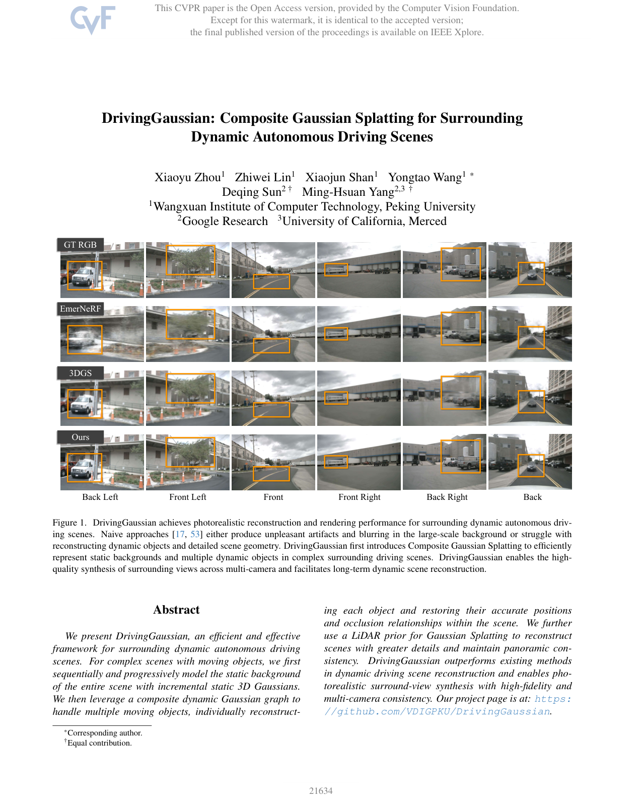
The article demonstrates and evaluates DrivingGaussian, a novel framework designed to reconstruct complex, large-scale dynamic driving scenes and synthesize photorealistic surrounding views. The framework decomposes scenes into static backgrounds and moving objects using sequential multi-sensor data, such as camera images and laser-based depth sensors (LiDAR).

The approach introduces two core components: an incremental model that builds the expansive static background sequentially across time, and a dynamic graph model that tracks, reconstructs, and positions moving objects individually. These representations are combined into a global model that correctly captures real-world occlusions. Furthermore, the method integrates LiDAR data to initialize geometric priors and improve spatial consistency across multi-camera setups. The authors evaluated this approach against leading neural radiance and Gaussian-based methods on established autonomous driving benchmarks, specifically nuScenes (multi-camera) and KITTI-360 (monocular).

The results show that the proposed method outperforms all existing state-of-the-art baselines. On the nuScenes benchmark, DrivingGaussian achieved superior image quality metrics, recording a peak signal-to-noise ratio (PSNR) of 28.74 dB—outperforming the leading competitor EmerNeRF (26.75 dB) and baseline 3D Gaussian Splatting (26.08 dB)—while reducing perceptual error (LPIPS) to 0.237 compared to over 0.298–0.311 for competing models. The method also proved effective in monocular settings on KITTI-360, leading the field with a PSNR of 25.62 dB. Ablation studies revealed that dynamic object modeling and static background decomposition are critical to performance, while LiDAR priors notably improve fine structural detail without requiring overly dense point clouds.

These findings mean that autonomous vehicle programs can generate realistic, multi-view dynamic simulations and test safety-critical edge cases—such as sudden pedestrian hazards—without high physical testing costs. By eliminating the need to estimate complex motion flows and addressing previous rendering artifacts, the framework improves simulation fidelity and developer safety validation pipelines.

Organizations developing autonomous systems should consider integrating composite Gaussian modeling pipelines into their simulation workflows for sensor validation and corner-case testing. However, the evaluation assumes the availability of bounding box detections (or tracking models) and calibrated sensor arrays. While the system demonstrates high resilience and functions well even with traditional point initialization instead of LiDAR, users should test performance in extreme optical conditions or unannotated environments before deploying it as a core component of production validation pipelines.

Cover for DrivingGaussian: Composite Gaussian Splatting for Surrounding Dynamic Autonomous Driving Scenes

Abstract

We present DrivingGaussian, an efficient and effective framework for surrounding dynamic autonomous driving scenes. For complex scenes with moving objects, we first sequentially and progressively model the static background of the entire scene with incremental static 3D Gaussians. We then leverage a composite dynamic Gaussian graph to handle multiple moving objects, individually reconstruct-ing each object and restoring their accurate positions and occlusion relationships within the scene. We further use a LiDAR prior for Gaussian Splatting to reconstruct scenes with greater details and maintain panoramic consistency. DrivingGaussian outperforms existing methods in dynamic driving scene reconstruction and enables photorealistic surround-view synthesis with high-fidelity and multi-camera consistency. Our project page is at: https://github.com/VDIGPKU/DrivingGaussian.

Table of Contents

  • 1. Introduction
  • 2. Related Work
  • 3. Method
  • 3.1. Composite Gaussian Splatting
  • 3.2. LiDAR Prior with surrounding views
  • 3.3. Global Rendering via Gaussian Splatting
  • 4. Experiments
  • 4.1. Datasets
  • 4.2. Implementation Details
  • 4.3. Results and Comparisons
  • 4.4. Ablation Study
  • 4.5. Corner Case Simulation
  • 5. Conclusion
  • 6. Acknowledgment
  • References

Knowls

  1. Knowl 1 — Composite Gaussian Splatting Framework

    model/method

    DrivingGaussian models complex, large-scale, surrounding dynamic autonomous driving scenes by decomposing the environment hierarchically into a static background and multiple dynamic foreground objects using sequential multi-sensor data (surrounding camera images and LiDAR).

    The complete scene representation, denoted as GcompG_{comp}, is formed by combining the incremental static 3D Gaussian field GsG_s with the dynamic instances structured in a dynamic Gaussian graph HH:

    Gcomp=∑H⟨O,Gd,M,P,A,T⟩+GsG_{comp} = \sum H\langle O, G_d, M, P, A, T \rangle + G_s

    where OO is the set of dynamic object instances, GdG_d represents the dynamic 3D Gaussians associated with each instance, MM contains the instance-to-world transformation matrices, PP denotes bounding box center positions, AA denotes bounding box orientations, and TT corresponds to timestamps.

    Global rendering uses differentiable splat-based rasterization where the 3D covariance matrix Σ\Sigma of each Gaussian is projected to 2D image coordinates as:

    Σ~=JEΣE⊤J⊤\widetilde{\Sigma} = J E \Sigma E^\top J^\top

    where JJ is the Jacobian matrix of the perspective projection and EE is the world-to-camera transformation matrix. Gaussians from future timestamps are initially invisible and incrementally incorporated into the scene under multi-view image supervision.

  2. Knowl 2 — Incremental Static 3D Gaussians

    model/method

    To prevent scale confusion and perspective artifacts caused by distant background elements moving relative to the ego vehicle over time, the static scene is partitioned chronologically into NN depth bins denoted as {bi}i=1N\{b_i\}_{i=1}^N, where each bin contains multi-camera images from one or more timestamps.

    The first bin b0b_0 initializes 3D Gaussians via LiDAR geometric priors (or Structure-from-Motion points) using an anisotropic Gaussian distribution:

    pb0(l∣μ,Σ)=exp⁡(−12(l−μ)⊤Σ−1(l−μ))p_{b_0}(l | \mu, \Sigma) = \exp\left(-\frac{1}{2}(l-\mu)^\top \Sigma^{-1}(l-\mu)\right)

    where l∈R3l \in \mathbb{R}^3 is a LiDAR point position, μ\mu is the mean of the points, and Σ∈R3×3\Sigma \in \mathbb{R}^{3 \times 3} is the anisotropic covariance matrix. Each Gaussian maintains a 3D position P(x,y,z)P(x, y, z), covariance Σ\Sigma, spherical harmonic color coefficients C(r,g,b)C(r, g, b), and opacity α\alpha.

    For subsequent bins b+1b+1, the 3D Gaussian centers P^b+1(Gs)\hat{P}_{b+1}(G_s) are updated by concatenating new local visible regions to the prior bin:

    P^b+1(Gs)=Pb(Gs)⋃(xb+1,yb+1,zb+1)\hat{P}_{b+1}(G_s) = P_b(G_s) \bigcup (x_{b+1}, y_{b+1}, z_{b+1})

    The accumulated color C^(Gs)\hat{C}(G_s) across all NN bins is rendered as:

    C^(Gs)=∑b=1NΓbαbCb,Γb=∏i=1b−1(1−αb)\hat{C}(G_s) = \sum_{b=1}^{N} \Gamma_b \alpha_b C_b, \quad \Gamma_b = \prod_{i=1}^{b-1} (1 - \alpha_b)

    where αb\alpha_b and CbC_b are the opacity and color of Gaussians at bin bb, and Γb\Gamma_b is the accumulated transmittance.

    To reconcile multi-camera sampling discrepancies between front and rear cameras, optimized pixel color C~\tilde{C} is produced via learnable weighted averaging during differential splatting ς\varsigma:

    C~=ς(Gs)∑ω(C^(Gs)∣R,T)\tilde{C} = \varsigma(G_s) \sum \omega(\hat{C}(G_s) | R, T)

    where ω\omega is a learnable weighting coefficient and [R,T][R, T] is the camera view-matrix.

  3. Knowl 3 — Composite Dynamic Gaussian Graph

    model/method

    Dynamic foreground objects in driving environments are modeled separately as nodes within a dynamic Gaussian graph H=⟨O,Gd,M,P,A,T⟩H = \langle O, G_d, M, P, A, T \rangle. Dynamic objects are extracted from 2D and 3D bounding boxes using Segment Anything Model (SAM) segmentation and tracking IDs.

    For each dynamic instance o∈Oo \in O, a dedicated set of dynamic Gaussians gi∈Gdg_i \in G_d is initialized and optimized in object-centric canonical coordinates. Transformation from the object canonical coordinate frame to the static background world coordinate frame is defined by:

    mo−1=Ro−1So−1m_o^{-1} = R_o^{-1} S_o^{-1}

    where Ro−1R_o^{-1} and So−1S_o^{-1} are the object's rotation and translation inverse matrices at time step t∈Tt \in T.

    To handle occlusions among multiple moving dynamic objects and maintain correct physical depth ordering relative to the camera, the opacity αo,t\alpha_{o, t} of dynamic Gaussians for object oo at time tt is dynamically modulated according to camera distance:

    αo,t=∑(pt−bo)2⋅cot⁡ao∥(bo∣Ro,So)−ρ∥2αp0\alpha_{o, t} = \sum \frac{(p_t - b_o)^2 \cdot \cot a_o}{\|(b_o | R_o, S_o) - \rho\|^2} \alpha_{p_0}

    where pt=(xt,yt,zt)p_t = (x_t, y_t, z_t) is the 3D center of the object's Gaussians, bob_o and ao=(θt,ϕt)a_o = (\theta_t, \phi_t) are the bounding box center and orientation, [Ro,So][R_o, S_o] is the object-to-world transformation matrix, ρ\rho denotes the optical center of the camera view, and αp0\alpha_{p_0} is the base Gaussian opacity.

  4. Knowl 4 — LiDAR Prior Projection and Multi-Camera Initialization

    model/method

    To provide accurate geometric initialization in sparse multi-camera setups, multi-frame LiDAR point sweeps LtL_t are merged into an aggregated scene point cloud LL. LiDAR points ls∈Ll_s \in L are projected onto image planes across surrounding cameras via known camera intrinsics K∈R3×3K \in \mathbb{R}^{3 \times 3} and extrinsics [Rti,Tti][R_t^i, T_t^i]:

    xpq=K[Rti⋅ls+Tti]x_p^q = K [R_t^i \cdot l_s + T_t^i]

    where xpqx_p^q is the 2D pixel coordinate in camera image ItiI_t^i. When a LiDAR point projects to multiple overlapping camera views, the correspondence with the shortest Euclidean distance to the image plane is retained, and color values are assigned.

    Dense bundle adjustment (DBA) is extended across multi-camera setups to refine the 3D positions of the LiDAR points before using them to initialize the positions and covariances of the 3D Gaussian Splatting models.

  5. Knowl 5 — Optimization Losses for Composite Gaussian Splatting

    equation

    DrivingGaussian optimizes the parameters δ\delta of the static and dynamic Gaussians using a joint objective composed of Tile Structural Similarity loss (LTSSIML_{TSSIM}), Robust photometric loss (LRobustL_{Robust}), and LiDAR geometric prior loss (LLiDARL_{LiDAR}):

    Ltotal(δ)=LTSSIM(δ)+LRobust(δ)+LLiDAR(δ)L_{total}(\delta) = L_{TSSIM}(\delta) + L_{Robust}(\delta) + L_{LiDAR}(\delta)

    The individual loss components are defined as:

    1. Tile Structural Similarity Loss over ZZ image tiles: LTSSIM(δ)=1−1Z∑z=1ZSSIM(Ψ(C^),Ψ(C))L_{TSSIM}(\delta) = 1 - \frac{1}{Z} \sum_{z=1}^{Z} \text{SSIM}(\Psi(\hat{C}), \Psi(C)) where Ψ(C^)\Psi(\hat{C}) is the rendered image tile and Ψ(C)\Psi(C) is the ground-truth image tile.

    2. Robust Photometric Loss for reducing outliers: LRobust(δ)=κ(∥I^−I∥2)L_{Robust}(\delta) = \kappa(\|\hat{I} - I\|_2) where I^\hat{I} is the synthesized image, II is the ground-truth image, and κ∈(0,1]\kappa \in (0, 1] is a parameter controlling error sensitivity.

    3. LiDAR Geometric Supervision Loss: LLiDAR(δ)=1s∑∥P(Gcomp)−Ls∥2L_{LiDAR}(\delta) = \frac{1}{s} \sum \|P(G_{comp}) - L_s\|^2 where P(Gcomp)P(G_{comp}) denotes the positions of the 3D Gaussians, LsL_s represents the corresponding target positions from the LiDAR prior point cloud, and ss is the number of supervised points.

  6. Knowl 6 — Reconstruction Performance on the nuScenes Dataset

    data/table

    DrivingGaussian evaluated novel view synthesis and dynamic reconstruction on the multi-camera nuScenes benchmark (6 cameras per frame) against state-of-the-art NeRF-based and 3DGS-based methods. Evaluated variants include Ours-S (initialized with Structure-from-Motion points) and Ours-L (initialized with LiDAR geometric priors).

    Methods Input PSNR ↑\uparrow SSIM ↑\uparrow LPIPS ↓\downarrow
    Instant-NGP Images 16.78 0.519 0.570
    NeRF+Time Images 17.54 0.565 0.532
    NSG Images 21.67 0.671 0.424
    Mip-NeRF Images 18.08 0.572 0.551
    Mip-NeRF360 Images 22.61 0.688 0.395
    Urban-NeRF Images + LiDAR 20.75 0.627 0.480
    S-NeRF Images + LiDAR 25.43 0.730 0.302
    SUDS Images + LiDAR 21.26 0.603 0.466
    EmerNeRF Images + LiDAR 26.75 0.760 0.311
    3DGS Images + SfM Points 26.08 0.717 0.298
    4DGS Images + SfM Points 19.79 0.622 0.473
    Ours-S Images + SfM Points 28.36 0.851 0.256
    Ours-L Images + LiDAR 28.74 0.865 0.237

    DrivingGaussian (Ours-L) outperforms all previous methods across all metrics, exceeding EmerNeRF by +1.99 dB PSNR and +0.105 SSIM. Even without LiDAR (Ours-S), it surpasses all existing methods, demonstrating the efficacy of composite Gaussian decomposition.

  7. Knowl 7 — Monocular Driving Scene Reconstruction on KITTI-360

    data/table

    Performance of DrivingGaussian on single-camera monocular view synthesis using the KITTI-360 benchmark compared to existing SOTA NeRF, mesh, graph, and Gaussian methods.

    Methods PSNR ↑\uparrow SSIM ↑\uparrow
    NeRF 21.94 0.781
    NSG 22.89 0.836
    Point-NeRF 21.54 0.793
    Mip-NeRF360 23.27 0.836
    SUDS 23.30 0.844
    DNMP 23.41 0.846
    3DGS 22.93 0.847
    Ours-S 25.18 0.862
    Ours-L 25.62 0.868

    Both Ours-S and Ours-L achieve state-of-the-art results on monocular input, demonstrating that DrivingGaussian generalizes effectively to single-camera driving setups.

  8. Knowl 8 — Ablation of Gaussian Initialization Priors and Point Density

    data/table

    Comparison of different 3D Gaussian initialization strategies and point counts on reconstruction quality on the nuScenes dataset. Initializations include random point distributions, COLMAP SfM points, pre-trained NeRF point clouds, and LiDAR point clouds at varying densities (LiDAR-600K downsampled, LiDAR-1M filtered/denoised, and LiDAR-2M raw points).

    Methods PSNR ↑\uparrow SSIM ↑\uparrow LPIPS ↓\downarrow
    Random-600K 22.18 0.653 0.424
    Random-1M 22.23 0.653 0.421
    SfM-600K 28.36 0.851 0.256
    NeRF-1M 28.51 0.858 0.251
    LiDAR-600K 28.49 0.854 0.245
    LiDAR-1M 28.74 0.865 0.237
    LiDAR-2M 28.78 0.867 0.237

    Random initialization performs poorly due to the lack of spatial geometry priors. LiDAR-1M (denoised and filtered) yields near-identical performance to the full LiDAR-2M while eliminating redundant points that hinder optimization.

  9. Knowl 9 — Ablation of Core Modules and Loss Functions in DrivingGaussian

    data/table

    Ablation study assessing the contribution of individual components of DrivingGaussian on the nuScenes dataset, including the Incremental Static 3D Gaussians (IS3G), Composite Dynamic Gaussian Graph (CDGG), and the loss terms LTSSIML_{TSSIM}, LRobustL_{Robust}, and LLiDARL_{LiDAR}.

    Model PSNR ↑\uparrow SSIM ↑\uparrow LPIPS ↓\downarrow
    w/o IS3G 27.72 0.771 0.295
    w/o CDGG 26.97 0.752 0.306
    w/o LTSSIML_{TSSIM} 27.88 0.783 0.280
    w/o LRobustL_{Robust} 28.05 0.814 0.271
    w/o LLiDARL_{LiDAR} 28.45 0.854 0.248
    Ours-S 28.36 0.851 0.256
    Ours-L 28.74 0.865 0.237

    Removing the Composite Dynamic Gaussian Graph (CDGG) results in the largest drop in PSNR (-1.77 dB) and SSIM (-0.113), indicating its essential role in reconstructing dynamic elements. Removing Incremental Static 3D Gaussians (IS3G) causes a -1.02 dB drop in PSNR and significant SSIM degradation (-0.094) due to background blur and multi-view artifacts.

Coverage note — None was omitted; all contributed models, methodologies, mathematical formulations, loss functions, benchmark evaluations on nuScenes and KITTI-360, and ablation experiments are included.

References

  1. 1.Chunge Bai, Ruijie Fu, and Xiang Gao. Colmap-pcd: An open-source tool for fine image-to-point cloud registration. arXiv preprint arXiv:2310.05504, 2023.
  2. 2.Jonathan T Barron, Ben Mildenhall, Matthew Tancik, Peter Hedman, Ricardo Martin-Brualla, and Pratul P Srinivasan. Mip-nerf: A multiscale representation for anti-aliasing neural radiance fields. In ICCV, pages 5855–5864, 2021.
  3. 3.Jonathan T Barron, Ben Mildenhall, Dor Verbin, Pratul P Srinivasan, and Peter Hedman. Mip-nerf 360: Unbounded anti-aliased neural radiance fields. In CVPR, pages 5470–5479, 2022.
  4. 4.Wenjing Bian, Zirui Wang, Kejie Li, Jia-Wang Bian, and Victor Adrian Prisacariu. Nope-nerf: Optimising neural radiance field with no pose prior. In CVPR, pages 4160–4169, 2023.
  5. 5.Holger Caesar, Varun Bankiti, Alex H Lang, Sourabh Vora, Venice Erin Liong, Qiang Xu, Anush Krishnan, Yu Pan, Giancarlo Baldan, and Oscar Beijbom. nuscenes: A multimodal dataset for autonomous driving. In CVPR, pages 11621–11631, 2020.
  6. 6.Holger Caesar, Juraj Kabzan, Kok Seang Tan, Whye Kit Fong, Eric Wolff, Alex Lang, Luke Fletcher, Oscar Beijbom, and Sammy Omari. nuplan: A closed-loop ml-based planning benchmark for autonomous vehicles. arXiv preprint arXiv:2106.11810, 2021.
  7. 7.Qi Cai, Yingwei Pan, Ting Yao, Chong-Wah Ngo, and Tao Mei. Objectfusion: Multi-modal 3d object detection with object-centric fusion. In ICCV, pages 18067–18076, 2023.
  8. 8.Ang Cao and Justin Johnson. Hexplane: A fast representation for dynamic scenes. In CVPR, pages 130–141, 2023.
  9. 9.Xuanyao Chen, Tianyuan Zhang, Yue Wang, Yilun Wang, and Hang Zhao. Futr3d: A unified sensor fusion framework for 3d detection. In CVPR, pages 172–181, 2023.
  10. 10.Sara Fridovich-Keil, Alex Yu, Matthew Tancik, Qinhong Chen, Benjamin Recht, and Angjoo Kanazawa. Plenoxels: Radiance fields without neural networks. In CVPR, pages 5501–5510, 2022.
  11. 11.Chen Gao, Ayush Saraf, Johannes Kopf, and Jia-Bin Huang. Dynamic view synthesis from dynamic monocular video. In ICCV, pages 5712–5721, 2021.
  12. 12.Stephan J Garbin, Marek Kowalski, Matthew Johnson, Jamie Shotton, and Julien Valentin. Fastnerf: High-fidelity neural rendering at 200fps. In ICCV, pages 14346–14355, 2021.
  13. 13.Vitor Guizilini, Igor Vasiljevic, Rares Ambrus, Greg Shakhnarovich, and Adrien Gaidon. Full surround monodepth from multiple cameras. RAL, pages 5397–5404, 2022.
  14. 14.Jianfei Guo, Nianchen Deng, Xinyang Li, Yeqi Bai, Botian Shi, Chiyu Wang, Chenjing Ding, Dongliang Wang, and Yikang Li. Streetsurf: Extending multi-view implicit surface reconstruction to street views. arXiv preprint arXiv:2306.04988, 2023.
  15. 15.Quentin Herau, Nathan Piasco, Moussab Bennehar, Luis Roldao, Dzmitry Tsishkou, Cyrille Migniot, Pascal Vasseur, ˜ and Cedric Demonceaux. Moisst: Multi-modal optimiza- ´ tion of implicit scene for spatiotemporal calibration. arXiv preprint arXiv:2303.03056, 2023.
  16. 16.Xin Huang, Qi Zhang, Ying Feng, Hongdong Li, Xuan Wang, and Qing Wang. Hdr-nerf: High dynamic range neural radiance fields. In CVPR, pages 18398–18408, 2022.
  17. 17.Bernhard Kerbl, Georgios Kopanas, Thomas Leimkuhler, ¨ and George Drettakis. 3D Gaussian splatting for real-time radiance field rendering. TOG, 42(4):1–14, 2023.
  18. 18.Alexander Kirillov, Eric Mintun, Nikhila Ravi, Hanzi Mao, Chloe Rolland, Laura Gustafson, Tete Xiao, Spencer Whitehead, Alexander C Berg, Wan-Yen Lo, et al. Segment anything. arXiv preprint arXiv:2304.02643, 2023.
  19. 19.Yuan Li, Zhi-Hao Lin, David Forsyth, Jia-Bin Huang, and Shenlong Wang. Climatenerf: Extreme weather synthesis in neural radiance field. In ICCV, pages 3227–3238, 2023.
  20. 20.Zhiqi Li, Wenhai Wang, Hongyang Li, Enze Xie, Chonghao Sima, Tong Lu, Yu Qiao, and Jifeng Dai. Bevformer: Learning bird’s-eye-view representation from multi-camera images via spatiotemporal transformers. In ECCV, pages 1– 18. Springer, 2022.
  21. 21.Tingting Liang, Hongwei Xie, Kaicheng Yu, Zhongyu Xia, Zhiwei Lin, Yongtao Wang, Tao Tang, Bing Wang, and Zhi Tang. Bevfusion: A simple and robust lidar-camera fusion framework. Advances in Neural Information Processing Systems, 35:10421–10434, 2022.
  22. 22.Yiyi Liao, Jun Xie, and Andreas Geiger. Kitti-360: A novel dataset and benchmarks for urban scene understanding in 2d and 3d. IEEE Transactions on Pattern Analysis and Machine Intelligence, 45(3):3292–3310, 2022.
  23. 23.Chen-Hsuan Lin, Wei-Chiu Ma, Antonio Torralba, and Simon Lucey. Barf: Bundle-adjusting neural radiance fields. In ICCV, pages 5741–5751, 2021.
  24. 24.Yu-Lun Liu, Chen Gao, Andreas Meuleman, Hung-Yu Tseng, Ayush Saraf, Changil Kim, Yung-Yu Chuang, Johannes Kopf, and Jia-Bin Huang. Robust dynamic radiance fields. In CVPR, pages 13–23, 2023.
  25. 25.Zhijian Liu, Haotian Tang, Alexander Amini, Xinyu Yang, Huizi Mao, Daniela L Rus, and Song Han. Bevfusion: Multi-task multi-sensor fusion with unified bird’s-eye view representation. In ICRA, pages 2774–2781. IEEE, 2023.
  26. 26.Fan Lu, Yan Xu, Guang Chen, Hongsheng Li, Kwan-Yee Lin, and Changjun Jiang. Urban radiance field representation with deformable neural mesh primitives. In ICCV, pages 465–476, 2023.
  27. 27.Jonathon Luiten, Georgios Kopanas, Bastian Leibe, and Deva Ramanan. Dynamic 3d gaussians: Tracking by persistent dynamic view synthesis. arXiv preprint arXiv:2308.09713, 2023.
  28. 28.Ricardo Martin-Brualla, Noha Radwan, Mehdi SM Sajjadi, Jonathan T Barron, Alexey Dosovitskiy, and Daniel Duckworth. Nerf in the wild: Neural radiance fields for unconstrained photo collections. In CVPR, pages 7210–7219, 2021.
  29. 29.Andreas Meuleman, Yu-Lun Liu, Chen Gao, Jia-Bin Huang, Changil Kim, Min H Kim, and Johannes Kopf. Progressively optimized local radiance fields for robust view synthesis. In CVPR, pages 16539–16548, 2023.
  30. 30.Ben Mildenhall, Pratul P Srinivasan, Matthew Tancik, Jonathan T Barron, Ravi Ramamoorthi, and Ren Ng. Nerf: Representing scenes as neural radiance fields for view synthesis. Communications of the ACM, pages 99–106, 2021.
  31. 31.Thomas Muller, Alex Evans, Christoph Schied, and Alexan- ¨ der Keller. Instant neural graphics primitives with a multiresolution hash encoding. TOG, 41(4):1–15, 2022.
  32. 32.Julian Ost, Fahim Mannan, Nils Thuerey, Julian Knodt, and Felix Heide. Neural scene graphs for dynamic scenes. In CVPR, pages 2856–2865, 2021.
  33. 33.Albert Pumarola, Enric Corona, Gerard Pons-Moll, and Francesc Moreno-Noguer. D-nerf: Neural radiance fields for dynamic scenes. In CVPR, pages 10318–10327, 2021.
  34. 34.Konstantinos Rematas, Andrew Liu, Pratul P Srinivasan, Jonathan T Barron, Andrea Tagliasacchi, Thomas Funkhouser, and Vittorio Ferrari. Urban radiance fields. In CVPR, pages 12932–12942, 2022.
  35. 35.Tianhe Ren, Shilong Liu, Ailing Zeng, Jing Lin, Kunchang Li, He Cao, Jiayu Chen, Xinyu Huang, Yukang Chen, Feng Yan, Zhaoyang Zeng, Hao Zhang, Feng Li, Jie Yang, Hongyang Li, Qing Jiang, and Lei Zhang. Grounded sam: Assembling open-world models for diverse visual tasks. arXiv preprint arXiv:2401.14159, 2024.
  36. 36.Viktor Rudnev, Mohamed Elgharib, William Smith, Lingjie Liu, Vladislav Golyanik, and Christian Theobalt. Nerf for outdoor scene relighting. In ECCV, pages 615–631. Springer, 2022.
  37. 37.Sara Sabour, Suhani Vora, Daniel Duckworth, Ivan Krasin, David J Fleet, and Andrea Tagliasacchi. Robustnerf: Ignoring distractors with robust losses. In CVPR, pages 20626– 20636, 2023.
  38. 38.Aron Schmied, Tobias Fischer, Martin Danelljan, Marc Pollefeys, and Fisher Yu. R3d3: Dense 3d reconstruction of dynamic scenes from multiple cameras. In ICCV, pages 3216–3226, 2023.
  39. 39.Johannes L Schonberger and Jan-Michael Frahm. Structure-from-motion revisited. In CVPR, pages 4104–4113, 2016.
  40. 40.Yeji Song, Chaerin Kong, Seoyoung Lee, Nojun Kwak, and Joonseok Lee. Towards efficient neural scene graphs by learning consistency fields. arXiv preprint arXiv:2210.04127, 2022.
  41. 41.Matthew Tancik, Vincent Casser, Xinchen Yan, Sabeek Pradhan, Ben Mildenhall, Pratul P Srinivasan, Jonathan T Barron, and Henrik Kretzschmar. Block-nerf: Scalable large scene neural view synthesis. In CVPR, pages 8248–8258, 2022.
  42. 42.Siyu Teng, Xuemin Hu, Peng Deng, Bai Li, Yuchen Li, Yunfeng Ai, Dongsheng Yang, Lingxi Li, Zhe Xuanyuan, Fenghua Zhu, et al. Motion planning for autonomous driving: The state of the art and future perspectives. IEEE Transactions on Intelligent Vehicles, 2023.
  43. 43.Haithem Turki, Deva Ramanan, and Mahadev Satyanarayanan. Mega-nerf: Scalable construction of large-scale nerfs for virtual fly-throughs. In CVPR, pages 12922–12931, 2022.
  44. 44.Haithem Turki, Jason Y Zhang, Francesco Ferroni, and Deva Ramanan. Suds: Scalable urban dynamic scenes. In CVPR, pages 12375–12385, 2023.
  45. 45.Zirui Wang, Shangzhe Wu, Weidi Xie, Min Chen, and Victor Adrian Prisacariu. Nerf–: Neural radiance fields without known camera parameters. arXiv preprint arXiv:2102.07064, 2021.
  46. 46.Zian Wang, Tianchang Shen, Jun Gao, Shengyu Huang, Jacob Munkberg, Jon Hasselgren, Zan Gojcic, Wenzheng Chen, and Sanja Fidler. Neural fields meet explicit geometric representations for inverse rendering of urban scenes. In CVPR, pages 8370–8380, 2023.
  47. 47.Guanjun Wu, Taoran Yi, Jiemin Fang, Lingxi Xie, Xiaopeng Zhang, Wei Wei, Wenyu Liu, Qi Tian, and Xinggang Wang. 4d gaussian splatting for real-time dynamic scene rendering. arXiv preprint arXiv:2310.08528, 2023.
  48. 48.Zirui Wu, Tianyu Liu, Liyi Luo, Zhide Zhong, Jianteng Chen, Hongmin Xiao, Chao Hou, Haozhe Lou, Yuantao Chen, Runyi Yang, et al. Mars: An instance-aware, modular and realistic simulator for autonomous driving. arXiv preprint arXiv:2307.15058, 2023.
  49. 49.Zeke Xie, Xindi Yang, Yujie Yang, Qi Sun, Yixiang Jiang, Haoran Wang, Yunfeng Cai, and Mingming Sun. S3im: Stochastic structural similarity and its unreasonable effectiveness for neural fields. In ICCV, pages 18024–18034, 2023.
  50. 50.Ziyang Xie, Junge Zhang, Wenye Li, Feihu Zhang, and Li Zhang. S-nerf: Neural radiance fields for street views. arXiv preprint arXiv:2303.00749, 2023.
  51. 51.Linning Xu, Yuanbo Xiangli, Sida Peng, Xingang Pan, Nanxuan Zhao, Christian Theobalt, Bo Dai, and Dahua Lin. Grid-guided neural radiance fields for large urban scenes. In CVPR, pages 8296–8306, 2023.
  52. 52.Qiangeng Xu, Zexiang Xu, Julien Philip, Sai Bi, Zhixin Shu, Kalyan Sunkavalli, and Ulrich Neumann. Point-nerf: Point-based neural radiance fields. In CVPR, pages 5438–5448, 2022.
  53. 53.Jiawei Yang, Boris Ivanovic, Or Litany, Xinshuo Weng, Seung Wook Kim, Boyi Li, Tong Che, Danfei Xu, Sanja Fidler, Marco Pavone, et al. Emernerf: Emergent spatial-temporal scene decomposition via self-supervision. arXiv preprint arXiv:2311.02077, 2023.
  54. 54.Ze Yang, Yun Chen, Jingkang Wang, Sivabalan Manivasagam, Wei-Chiu Ma, Anqi Joyce Yang, and Raquel Urtasun. Unisim: A neural closed-loop sensor simulator. In CVPR, pages 1389–1399, 2023.
  55. 55.Ziyi Yang, Xinyu Gao, Wen Zhou, Shaohui Jiao, Yuqing Zhang, and Xiaogang Jin. Deformable 3d gaussians for high-fidelity monocular dynamic scene reconstruction. arXiv preprint arXiv:2309.13101, 2023.
  56. 56.MI Zhenxing and Dan Xu. Switch-nerf: Learning scene decomposition with mixture of experts for large-scale neural radiance fields. In The Eleventh International Conference on Learning Representations, 2022.

Citation

MLA
Zhou, X., et al. “DrivingGaussian: Composite Gaussian Splatting for Surrounding Dynamic Autonomous Driving Scenes”. arXiv, 2023, http://arxiv.org/abs/2312.07920v3.
APA
Zhou, X., Lin, Z., Shan, X., Wang, Y., Sun, D., & Yang, M.-H. (2023). DrivingGaussian: Composite Gaussian Splatting for Surrounding Dynamic Autonomous Driving Scenes. arXiv. http://arxiv.org/abs/2312.07920v3
Chicago
Zhou, X., Z. Lin, X. Shan, Y. Wang, D. Sun, and M.-H. Yang. 2023. “DrivingGaussian: Composite Gaussian Splatting for Surrounding Dynamic Autonomous Driving Scenes”. arXiv. http://arxiv.org/abs/2312.07920v3.
Harvard
Zhou, X. et al. (2023) “DrivingGaussian: Composite Gaussian Splatting for Surrounding Dynamic Autonomous Driving Scenes”, arXiv [Preprint]. Available at: http://arxiv.org/abs/2312.07920v3.
Vancouver
1. Zhou X, Lin Z, Shan X, Wang Y, Sun D, Yang M-H (2023) DrivingGaussian: Composite Gaussian Splatting for Surrounding Dynamic Autonomous Driving Scenes. arXiv

BibTeX

@article{zhou2023drivinggaussian,
  title = {DrivingGaussian: Composite Gaussian Splatting for Surrounding Dynamic Autonomous Driving Scenes},
  author = {Zhou, Xiaoyu and Lin, Zhiwei and Shan, Xiaojun and Wang, Yongtao and Sun, Deqing and Yang, Ming-Hsuan},
  year = {2023},
  journal = {arXiv},
  url = {http://arxiv.org/abs/2312.07920v3},
  eprint = {2312.07920}
}
Metadata:arXiv

Source Code

This paper has an official code repository available. Click below to access the source code.

View Repository

Access the Paper

This paper is available from its original source. Click below to access the PDF.

Open PDF
License: IEEE