How Does Batch Normalization Help Optimization?

Shibani SanturkarDimitris TsiprasAndrew IlyasAleksander Madry

article2018NeurIPS1,769 citations

Demonstrates that Batch Normalization accelerates deep network training not by reducing internal covariate shift, but by smoothing the loss surface to induce more predictable and stable gradients.

Listen

Deep neural networks are central to modern artificial intelligence applications, yet the fundamental mechanisms behind standard training techniques remain poorly understood. A prominent example is Batch Normalization, a ubiquitous technique introduced to speed up and stabilize model training. For years, the prevailing consensus held that Batch Normalization succeeds because it reduces internal covariate shift—the continuous, destabilizing change in the distribution of layer inputs during training. Understanding whether this assumption is true is critical for designing more efficient architectures and optimization methods.

The main objective of the article is to rigorously evaluate whether the reduction of internal covariate shift truly explains the effectiveness of Batch Normalization, and to identify the actual underlying mathematical and empirical reasons for its success.

To investigate this, the authors conducted empirical experiments using standard convolutional and deep linear networks on image classification tasks, alongside rigorous mathematical analysis. They evaluated training behavior when deliberately injecting time-varying, non-zero noise after normalization layers to forcefully induce input distributional instability. They also formulated a direct, gradient-based metric to quantify cross-layer dependency shifts, and derived theoretical bounds regarding the smoothness and stability of the network's optimization landscape with and without normalization.

The article establishes several key findings that overturn conventional assumptions. First, stabilizing layer input distributions has little to no connection with training performance; models with injected distribution instability trained just as quickly and accurately as standard Batch Normalization models, while unnormalized models with identical noise failed completely. Second, Batch Normalization does not necessarily reduce internal covariate shift from an optimization perspective, often showing similar or higher shift compared to standard networks. Third, the true mechanism driving success is landscape smoothing: Batch Normalization reparametrizes the optimization problem to make both the loss function and its gradients significantly smoother, improving gradient predictability by up to nearly two orders of magnitude in early training. Finally, this smoothing effect is not unique to Batch Normalization; alternative norm-based scaling strategies achieved comparable or superior optimization gains despite inducing severe distributional shifts.

These findings imply that engineering efforts previously aimed at controlling activation distributions may be misdirected. The practical value of normalization lies in enabling larger, more stable learning steps without encountering sudden gradient explosions or vanishing gradients. This significantly lowers hyperparameter tuning costs, shortens development timelines, and ensures robust training convergence across broader operational settings.

Moving forward, machine learning teams and researchers should shift focus from preserving distributional stability toward designing normalization schemes that prioritize landscape smoothness and computational efficiency. Organizations should explore alternative normalization designs across various model architectures to identify lighter or faster alternatives. Further empirical work is warranted to examine how these smoothing mechanisms influence final generalization performance and convergence toward flatter optima across broader model classes.

arXiv: 1805.11604
  • Paper: Group Normalization, Yuxin Wu et al. (2018). Introduces Group Normalization to overcome mini-batch dependency limitations while maintaining the optimization stabilization benefits highlighted by the source.
  • Paper: Root Mean Square Layer Normalization, Biao Zhang et al. (2019). Simplifies layer normalization by relying only on root mean square scaling, building on insights that mean-centering and covariate shift reduction are secondary to scaling-induced optimization benefits.
  • Paper: On Layer Normalization in the Transformer Architecture, Ruibin Xiong et al. (2020). Investigates the placement of normalization layers in Transformers and analyzes gradient variance and optimization stability at initialization.
  • Paper: Averaging Weights Leads to Wider Optima and Better Generalization, Pavel Izmailov et al. (2018). Explores how trajectory averaging helps navigate smoother, wider loss basins for better generalization in deep neural networks.
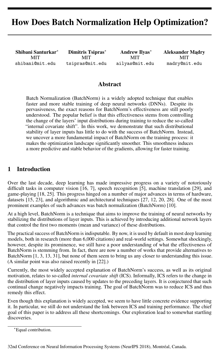
Cover for How Does Batch Normalization Help Optimization?

Abstract

Batch Normalization (BatchNorm) is a widely adopted technique that enables faster and more stable training of deep neural networks (DNNs). Despite its pervasiveness, the exact reasons for BatchNorm's effectiveness are still poorly understood. The popular belief is that this effectiveness stems from controlling the change of the layers' input distributions during training to reduce the so-called "internal covariate shift". In this work, we demonstrate that such distributional stability of layer inputs has little to do with the success of BatchNorm. Instead, we uncover a more fundamental impact of BatchNorm on the training process: it makes the optimization landscape significantly smoother. This smoothness induces a more predictive and stable behavior of the gradients, allowing for faster training.

Table of Contents

  • 1 Introduction
  • 2 Batch normalization and internal covariate shift
  • 2.1 Does BatchNorm’s performance stem from controlling internal covariate shift?
  • 2.2 Is BatchNorm reducing internal covariate shift?
  • 3 Why does BatchNorm work?
  • 3.1 The smoothing effect of BatchNorm
  • 3.2 Exploration of the optimization landscape
  • 3.3 Is BatchNorm the best (only?) way to smoothen the landscape?
  • 4 Theoretical Analysis
  • 4.1 Setup
  • 4.2 Theoretical Results
  • 5 Related work
  • 6 Conclusions
  • References
  • A Experimental Setup
  • A.1 Models
  • A.2 Details
  • A.2.1 “Noisy” BatchNorm Layers
  • A.2.2 Loss Landscape
  • B Omitted Figures
  • C Proofs
  • C.1 Useful facts and setup
  • C.2 Lipschitzness proofs

Knowls

  1. Knowl 1 — Loss Lipschitzness Bound for Batch Normalization

    theoretical result

    Let WW be a fully connected layer with weights WijW_{ij}, receiving input batch X=(x1,…,xm)X = (x_1, \dots, x_m) of size mm, and producing activations yj=WjX∈Rmy_j = W_j X \in \mathbb{R}^m for output unit jj. Let L\mathcal{L} be an arbitrary differentiable loss function of the unnormalized network, and let L^\widehat{\mathcal{L}} be the loss of the network when a Batch Normalization (BN) layer is inserted after WW, computing standardized activations y^j=(yj−μj)/σj\hat{y}_j = (y_j - \mu_j)/\sigma_j (where μj\mu_j is the batch mean and σj\sigma_j is the batch standard deviation) followed by linear scaling zj=γy^j+βz_j = \gamma \hat{y}_j + \beta with constant parameters γ,β\gamma, \beta.

    The gradient norm of the loss with respect to the pre-activation outputs yjy_j in the batch-normalized network is upper-bounded by:

    ∥∇yjL^∥2≤γ2σj2(∥∇yjL∥2−1m⟨1,∇yjL⟩2−1m⟨∇yjL,y^j⟩2)\|\nabla_{y_j} \widehat{\mathcal{L}}\|^2 \le \frac{\gamma^2}{\sigma_j^2} \left( \|\nabla_{y_j} \mathcal{L}\|^2 - \frac{1}{m} \langle \mathbf{1}, \nabla_{y_j} \mathcal{L} \rangle^2 - \frac{1}{m} \langle \nabla_{y_j} \mathcal{L}, \hat{y}_j \rangle^2 \right)

    where 1∈Rm\mathbf{1} \in \mathbb{R}^m is the all-ones vector. This bound demonstrates an additive reduction in the gradient norm whenever the mean of the unnormalized gradient deviates from zero (⟨1,∇yjL⟩≠0\langle \mathbf{1}, \nabla_{y_j} \mathcal{L} \rangle \ne 0) or whenever the unnormalized gradient correlates with normalized activations y^j\hat{y}_j (⟨∇yjL,y^j⟩≠0\langle \nabla_{y_j} \mathcal{L}, \hat{y}_j \rangle \ne 0). In addition, large batch variance σj\sigma_j provides multiplicative reduction via γ2/σj2\gamma^2 / \sigma_j^2, improving the Lipschitz constant of the loss landscape.

  2. Knowl 2 — Hessian Smoothness and Gradient Predictability Bound for Batch Normalization

    theoretical result

    Let g^j=∇yjL\hat{g}_j = \nabla_{y_j} \mathcal{L} and Hjj=∂2L∂yj∂yjH_{jj} = \frac{\partial^2 \mathcal{L}}{\partial y_j \partial y_j} be the gradient and Hessian of the unnormalized network loss L\mathcal{L} with respect to layer outputs yj∈Rmy_j \in \mathbb{R}^m over a mini-batch of size mm. For the batch-normalized network with loss L^\widehat{\mathcal{L}}, normalized activations y^j=(yj−μj)/σj\hat{y}_j = (y_j - \mu_j)/\sigma_j, batch standard deviation σj\sigma_j, and scaling parameter γ\gamma, the second-order directional derivative along the normalized gradient direction satisfies:

    (∇yjL^)⊤∂2L^∂yj∂yj(∇yjL^)≤γ2σj2(∂L^∂yj)⊤Hjj(∂L^∂yj)−γmσj2⟨g^j,y^j⟩∥∂L^∂yj∥2(\nabla_{y_j} \widehat{\mathcal{L}})^\top \frac{\partial^2 \widehat{\mathcal{L}}}{\partial y_j \partial y_j} (\nabla_{y_j} \widehat{\mathcal{L}}) \le \frac{\gamma^2}{\sigma_j^2} \left( \frac{\partial \widehat{\mathcal{L}}}{\partial y_j} \right)^\top H_{jj} \left( \frac{\partial \widehat{\mathcal{L}}}{\partial y_j} \right) - \frac{\gamma}{m \sigma_j^2} \langle \hat{g}_j, \hat{y}_j \rangle \left\| \frac{\partial \widehat{\mathcal{L}}}{\partial y_j} \right\|^2

    Furthermore, if HjjH_{jj} preserves the relative norms of g^j\hat{g}_j and ∇yjL^\nabla_{y_j} \widehat{\mathcal{L}}, this yields:

    (∇yjL^)⊤∂2L^∂yj∂yj(∇yjL^)≤γ2σj2(g^j⊤Hjjg^j−1mγ⟨g^j,y^j⟩∥∂L^∂yj∥2)(\nabla_{y_j} \widehat{\mathcal{L}})^\top \frac{\partial^2 \widehat{\mathcal{L}}}{\partial y_j \partial y_j} (\nabla_{y_j} \widehat{\mathcal{L}}) \le \frac{\gamma^2}{\sigma_j^2} \left( \hat{g}_j^\top H_{jj} \hat{g}_j - \frac{1}{m \gamma} \langle \hat{g}_j, \hat{y}_j \rangle \left\| \frac{\partial \widehat{\mathcal{L}}}{\partial y_j} \right\|^2 \right)

    When the unnormalized loss is locally convex (Hjj⪰0H_{jj} \succeq 0) and the negative gradient points towards the minimum (⟨g^j,y^j⟩>0\langle \hat{g}_j, \hat{y}_j \rangle > 0), the quadratic variation in the gradient direction is strictly suppressed, resulting in higher gradient predictiveness (better effective β\beta-smoothness).

  3. Knowl 3 — Minimax Bound on Weight-Space Loss Lipschitzness

    theoretical result

    Let WW denote the weights of a fully connected layer in a neural network, and consider mini-batch inputs XX bounded such that ∥X∥≤λ\|X\| \le \lambda. Let L\mathcal{L} be the unnormalized network loss and L^\widehat{\mathcal{L}} be the batch-normalized network loss with activation standard deviation σj\sigma_j, affine scale parameter γ\gamma, and batch size mm. Define the worst-case squared Frobenius gradient norms with respect to layer weights as:

    gj=max⁡∥X∥≤λ∥∇WL∥2,g^j=max⁡∥X∥≤λ∥∇WL^∥2g_j = \max_{\|X\| \le \lambda} \|\nabla_W \mathcal{L}\|^2, \quad \hat{g}_j = \max_{\|X\| \le \lambda} \|\nabla_W \widehat{\mathcal{L}}\|^2

    Then the worst-case weight-space Lipschitz constant for the batch-normalized network is bounded by:

    g^j≤γ2σj2(gj2−mμgj2−λ2⟨∇yjL,y^j⟩2)\hat{g}_j \le \frac{\gamma^2}{\sigma_j^2} \left( g_j^2 - m \mu_{g_j}^2 - \lambda^2 \langle \nabla_{y_j} \mathcal{L}, \hat{y}_j \rangle^2 \right)

    where μgj\mu_{g_j} is the mean of ∇yjL\nabla_{y_j} \mathcal{L} over the batch. This establishes that the Lipschitz smoothness benefits derived in activation space translate directly to worst-case upper bounds on the gradient norms with respect to layer weights WW.

  4. Knowl 4 — Optimization-Based Definition of Internal Covariate Shift

    definition

    Let L\mathcal{L} denote the loss function of a kk-layer neural network, let W1(t),…,Wk(t)W_1^{(t)}, \dots, W_k^{(t)} denote the weight parameters of each layer at training step tt, and let (x(t),y(t))(x^{(t)}, y^{(t)}) denote the training mini-batch used at time tt.

    The internal covariate shift (ICS) experienced by layer ii at time tt is defined as the ℓ2\ell_2 difference between its parameter gradient before and after the parameters of preceding layers are updated:

    ICSt,i=∥Gt,i−Gt,i′∥2\text{ICS}_{t,i} = \|G_{t,i} - G'_{t,i}\|_2

    where

    ight)$$ is the standard simultaneous gradient update, and $$G'_{t,i} = \nabla_{W_i^{(t)}} \mathcal{L}\left(W_1^{(t+1)}, \dots, W_{i-1}^{(t+1)}, W_i^{(t)}, W_{i+1}^{(t)}, \dots, W_k^{(t)}; x^{(t)}, y^{(t)} ight)$$ is the gradient for layer $i$ re-evaluated after updating all preceding layers $1, \dots, i-1$ to their new values $W_1^{(t+1)}, \dots, W_{i-1}^{(t+1)}$. The difference $\|G_{t,i} - G'_{t,i}\|_2$ and the cosine angle between $G_{t,i}$ and $G'_{t,i}$ quantify the change in the optimization landscape for layer $i$ caused specifically by cross-layer parameter updates.
  5. Knowl 5 — BatchNorm Training Resilience Under Explicit Activation Noise Injection

    empirical result

    To test whether the performance benefits of BatchNorm arise from stabilizing the mean and variance of layer inputs, independent time-varying noise sampled from distributions with non-zero mean and non-unit variance was added to each normalized activation directly after every BatchNorm layer in a VGG network on CIFAR-10.

    Key observations include:

    1. The noise injection causes severe, continual distributional instability at every training step across units and layers, yielding qualitatively higher variance in layer input distributions than even standard, unnormalized networks.
    2. Despite this deliberate covariate shift, the 'noisy' BatchNorm network matches the training speed and accuracy of standard BatchNorm networks almost identically.
    3. Adding identical noise to standard networks without BatchNorm causes training to fail entirely.

    These results show that distributional stability of layer inputs is not the cause of the training performance gains enabled by BatchNorm.

  6. Knowl 6 — Empirical Measurement of Gradient ICS in Standard and BatchNorm Networks

    empirical result

    Measuring optimization-based internal covariate shift (ICS)—evaluated via the ℓ2\ell_2 gradient difference ∥Gt,i−Gt,i′∥2\|G_{t,i} - G'_{t,i}\|_2 and the cosine angle between Gt,iG_{t,i} and Gt,i′G'_{t,i} before and after updating preceding layers—demonstrates that BatchNorm does not reduce ICS:

    1. In Deep Linear Networks (DLN, 25 layers) trained with full-batch gradient descent, standard unnormalized networks maintain near-zero ℓ2\ell_2 gradient differences and a gradient cosine angle close to 11 (minimal ICS) throughout training, whereas BatchNorm networks exhibit substantially higher ℓ2\ell_2 gradient differences and cosine angles near 00 (high ICS).
    2. In VGG networks on CIFAR-10, BatchNorm models exhibit comparable or larger gradient discrepancies across intermediate layers than standard networks.
    3. In both architectures, BatchNorm networks converge significantly faster and attain lower training loss despite experiencing equal or greater optimization ICS than vanilla networks.
  7. Knowl 7 — Optimization Landscape Smoothening by Batch Normalization

    empirical result

    Empirical evaluation of loss landscapes along the gradient direction across VGG and deep linear networks demonstrates that BatchNorm fundamentally smooths optimization via three specific mechanisms:

    1. Loss Variation (Lipschitzness): Vanilla deep networks exhibit drastic, erratic swings in loss value when moving in the gradient direction, whereas BatchNorm networks restrict loss changes to a narrow, well-behaved band.
    2. Gradient Predictiveness: The ℓ2\ell_2 distance between the loss gradient at the current weights ∇L(W)\nabla \mathcal{L}(W) and gradients at steps along that direction ∇L(W−η∇L(W))\nabla \mathcal{L}(W - \eta \nabla \mathcal{L}(W)) is up to two orders of magnitude smaller in BatchNorm networks, confirming that gradient directions remain stable and predictive over large steps.
    3. Effective β\beta-Smoothness: The maximum normalized gradient change along the gradient path (max⁡η∥∇L(W)−∇L(W−η∇L)∥2/∥η∇L∥2\max_{\eta} \|\nabla \mathcal{L}(W) - \nabla \mathcal{L}(W - \eta \nabla \mathcal{L})\|_2 / \|\eta \nabla \mathcal{L}\|_2) is substantially smaller and more uniform across training steps for BatchNorm.

    This landscape smoothening enables the use of significantly higher learning rates without encountering vanishing or exploding gradients.

  8. Knowl 8 — Preservation of Optimization Minima Under BatchNorm Reparametrization

    theoretical result

    For any input data matrix XX and standard fully connected network parameter configuration WW, there exists an equivalent Batch Normalization layer configuration (W,γ,β)(W, \gamma, \beta) that yields identical layer outputs zj=yj=WjXz_j = y_j = W_j X for all units jj by setting the affine scaling parameters to γ=σj\gamma = \sigma_j (the mini-batch standard deviation of yjy_j) and shift parameters to β=μj\beta = \mu_j (the mini-batch mean of yjy_j).

    Consequently, the addition of BatchNorm is a reparametrization of the optimization problem rather than a restriction of model capacity, and every local and global minimum present in the vanilla loss landscape is preserved within the batch-normalized loss landscape.

  9. Knowl 9 — Optimization Landscape Smoothing Across Alternative Lp-Norm Normalizations

    empirical result

    Evaluating alternative normalization schemes that center activation means to zero and normalize by the average ℓp\ell_p-norm (for p∈{1,2,∞}p \in \{1, 2, \infty\}) instead of mini-batch standard deviation demonstrates that landscape smoothing is not unique to standard ℓ2\ell_2 BatchNorm:

    1. On VGG and deep linear networks trained on CIFAR-10, ℓ1\ell_1, ℓ2\ell_2, and ℓ∞\ell_\infty normalization schemes all match or exceed the training acceleration and final accuracy of standard BatchNorm (with ℓ1\ell_1-normalization outperforming BatchNorm on deep linear networks).
    2. Normalization with p=1p = 1 and p=∞p = \infty produces non-Gaussian, skewed activation distributions that fail to stabilize distribution moments or control covariate shift, yet still achieve the same landscape smoothening (improved gradient predictiveness and lower effective β\beta-smoothness).

    This indicates that training acceleration across normalization methods is driven by optimization landscape smoothing rather than Gaussian moment control.

  10. Knowl 10 — Proximity of Parameter Initialization to Local Optima Under Batch Normalization

    theoretical result

    Let W∗W^* and W^∗\widehat{W}^* denote the sets of local optima for layer weights in an unnormalized network and a batch-normalized network, respectively. For any initial weight configuration W0W_0, let W∗W^* and W^∗\widehat{W}^* be the closest local optima in the respective parameter spaces. If ⟨W0,W∗⟩>0\langle W_0, W^* \rangle > 0, then:

    ∥W0−W^∗∥2≤∥W0−W∗∥2−1∥W∗∥2(∥W∗∥2−⟨W∗,W0⟩)2\|W_0 - \widehat{W}^*\|^2 \le \|W_0 - W^*\|^2 - \frac{1}{\|W^*\|^2} \left( \|W^*\|^2 - \langle W^*, W_0 \rangle \right)^2

    Because the BatchNorm reparametrization is scale-invariant with respect to layer weights, each unnormalized optimum corresponds to a continuous ray of optima in the batch-normalized weight space, ensuring that the Euclidean distance from an initialization W0W_0 to the nearest optimum is strictly smaller than or equal to that of the vanilla network.

Coverage note — No substantial contributed material was omitted; minor appendix-only technical lemmas (such as minimax gradient predictiveness bound Theorem C.1) and hyperparameter sensitivity figures from the supplementary materials were subsumed into the main landscape smoothness and theoretical bound knowls.

References

  1. 1.Jimmy Lei Ba, Jamie Ryan Kiros, and Geoffrey E Hinton. Layer normalization. arXiv preprint arXiv:1607.06450, 2016.
  2. 2.David Balduzzi, Marcus Frean, Lennox Leary, JP Lewis, Kurt Wan-Duo Ma, and Brian McWilliams. The shattered gradients problem: If resnets are the answer, then what is the question? arXiv preprint arXiv:1702.08591, 2017.
  3. 3.Djork-Arné Clevert, Thomas Unterthiner, and Sepp Hochreiter. Fast and accurate deep network learning by exponential linear units (elus). arXiv preprint arXiv:1511.07289, 2015.
  4. 4.Xavier Glorot and Yoshua Bengio. Understanding the difficulty of training deep feedforward neural networks. In Proceedings of the thirteenth international conference on artificial intelligence and statistics, pages 249–256, 2010.
  5. 5.Alex Graves, Abdel-rahman Mohamed, and Geoffrey Hinton. Speech recognition with deep recurrent neural networks. In Acoustics, speech and signal processing (icassp), 2013 ieee international conference on, pages 6645–6649. IEEE, 2013.
  6. 6.Moritz Hardt and Tengyu Ma. Identity matters in deep learning. arXiv preprint arXiv:1611.04231, 2016.
  7. 7.Kaiming He, Xiangyu Zhang, Shaoqing Ren, and Jian Sun. Deep residual learning for image recognition. In Proceedings of the IEEE Conference on Computer Vision and Pattern Recognition, 2016.
  8. 8.Sepp Hochreiter and Jürgen Schmidhuber. Flat minima. Neural Computation, 9(1):1–42, 1997.
  9. 9.Daniel Jiwoong Im, Michael Tao, and Kristin Branson. An empirical analysis of deep network loss surfaces. arXiv preprint arXiv:1612.04010, 2016.
  10. 10.Sergey Ioffe and Christian Szegedy. Batch normalization: Accelerating deep network training by reducing internal covariate shift. arXiv preprint arXiv:1502.03167, 2015.
  11. 11.Nitish Shirish Keskar, Dheevatsa Mudigere, Jorge Nocedal, Mikhail Smelyanskiy, and Ping Tak Peter Tang. On large-batch training for deep learning: Generalization gap and sharp minima. arXiv preprint arXiv:1609.04836, 2016.
  12. 12.Diederik P Kingma and Jimmy Ba. Adam: A method for stochastic optimization. arXiv preprint arXiv:1412.6980, 2014.
  13. 13.Günter Klambauer, Thomas Unterthiner, Andreas Mayr, and Sepp Hochreiter. Self-normalizing neural networks. In Advances in Neural Information Processing Systems, pages 972–981, 2017.
  14. 14.Jonas Kohler, Hadi Daneshmand, Aurelien Lucchi, Ming Zhou, Klaus Neymeyr, and Thomas Hofmann. Towards a theoretical understanding of batch normalization. arXiv preprint arXiv:1805.10694, 2018.
  15. 15.Alex Krizhevsky and Geoffrey Hinton. Learning multiple layers of features from tiny images. 2009.
  16. 16.Alex Krizhevsky, Ilya Sutskever, and Geoffrey E Hinton. Imagenet classification with deep convolutional neural networks. In Advances in neural information processing systems, pages 1097–1105, 2012.
  17. 17.Hao Li, Zheng Xu, Gavin Taylor, and Tom Goldstein. Visualizing the loss landscape of neural nets. arXiv preprint arXiv:1712.09913, 2017.
  18. 18.Volodymyr Mnih, Koray Kavukcuoglu, David Silver, Andrei A Rusu, Joel Veness, Marc G Bellemare, Alex Graves, Martin Riedmiller, Andreas K Fidjeland, Georg Ostrovski, et al. Human-level control through deep reinforcement learning. Nature, 518(7540):529, 2015.
  19. 19.Ari S Morcos, David GT Barrett, Neil C Rabinowitz, and Matthew Botvinick. On the importance of single directions for generalization. arXiv preprint arXiv:1803.06959, 2018.
  20. 20.Vinod Nair and Geoffrey E Hinton. Rectified linear units improve restricted boltzmann machines. In Proceedings of the 27th international conference on machine learning (ICML-10), 2010.
  21. 21.Yurii Nesterov. Introductory lectures on convex optimization: A basic course, volume 87. Springer Science & Business Media, 2013.
  22. 22.Ali Rahimi and Ben Recht. Back when we were kids. In NIPS Test-of-Time Award Talk, 2017.
  23. 23.Olga Russakovsky, Jia Deng, Hao Su, Jonathan Krause, Sanjeev Satheesh, Sean Ma, Zhiheng Huang, Andrej Karpathy, Aditya Khosla, Michael Bernstein, Alexander C. Berg, and Li Fei-Fei. ImageNet Large Scale Visual Recognition Challenge. International Journal of Computer Vision (IJCV), 115(3), 2015.
  24. 24.Tim Salimans and Diederik P Kingma. Weight normalization: A simple reparameterization to accelerate training of deep neural networks. In Advances in Neural Information Processing Systems, 2016.
  25. 25.David Silver, Aja Huang, Chris J Maddison, Arthur Guez, Laurent Sifre, George Van Den Driessche, Julian Schrittwieser, Ioannis Antonoglou, Veda Panneershelvam, Marc Lanctot, et al. Mastering the game of go with deep neural networks and tree search. nature, 529(7587):484–489, 2016.
  26. 26.Karen Simonyan and Andrew Zisserman. Very deep convolutional networks for large-scale image recognition. arXiv preprint arXiv:1409.1556, 2014.
  27. 27.Nitish Srivastava, Geoffrey Hinton, Alex Krizhevsky, Ilya Sutskever, and Ruslan Salakhutdinov. Dropout: A simple way to prevent neural networks from overfitting. The Journal of Machine Learning Research, 15(1), 2014.
  28. 28.Ilya Sutskever, James Martens, George Dahl, and Geoffrey Hinton. On the importance of initialization and momentum in deep learning. In International conference on machine learning, 2013.
  29. 29.Ilya Sutskever, Oriol Vinyals, and Quoc V Le. Sequence to sequence learning with neural networks. In Advances in neural information processing systems, pages 3104–3112, 2014.
  30. 30.Dmitry Ulyanov, Andrea Vedaldi, and Victor Lempitsky. Instance normalization: The missing ingredient for fast stylization. arXiv preprint arXiv:1607.08022, 2016.
  31. 31.Yuxin Wu and Kaiming He. Group normalization. arXiv preprint arXiv:1803.08494, 2018.

Citation

MLA
Santurkar, S., et al. “How Does Batch Normalization Help Optimization?”. arXiv, 2018, http://arxiv.org/abs/1805.11604v5.
APA
Santurkar, S., Tsipras, D., Ilyas, A., & Madry, A. (2018). How Does Batch Normalization Help Optimization?. arXiv. http://arxiv.org/abs/1805.11604v5
Chicago
Santurkar, S., D. Tsipras, A. Ilyas, and A. Madry. 2018. “How Does Batch Normalization Help Optimization?”. arXiv. http://arxiv.org/abs/1805.11604v5.
Harvard
Santurkar, S. et al. (2018) “How Does Batch Normalization Help Optimization?”, arXiv [Preprint]. Available at: http://arxiv.org/abs/1805.11604v5.
Vancouver
1. Santurkar S, Tsipras D, Ilyas A, Madry A (2018) How Does Batch Normalization Help Optimization?. arXiv

BibTeX

@article{santurkar2018how,
  title = {How Does Batch Normalization Help Optimization?},
  author = {Santurkar, Shibani and Tsipras, Dimitris and Ilyas, Andrew and Madry, Aleksander},
  year = {2018},
  journal = {arXiv},
  url = {http://arxiv.org/abs/1805.11604v5},
  eprint = {1805.11604}
}
Metadata:arXiv

Access the Paper

This paper is available from its original source. Click below to access the PDF.

Open PDF
License: Authors