Visualizing the Loss Landscape of Neural Nets

Hao LiZheng XuGavin TaylorT. Goldstein

article2017NeurIPS2,425 citations

Introduces a filter-normalized visualization technique that reveals how network architectures like skip connections smooth high-dimensional loss surfaces to improve training stability and generalization.

Listen

Deep neural networks are central to modern artificial intelligence applications, yet understanding why certain model architectures train reliably and generalize well to new data remains a critical challenge. Historically, evaluating high-dimensional neural loss functions has relied largely on theoretical approximations or flawed visualization techniques that produce misleading results due to network scale invariance.

The article sets out to establish an accurate method for visualizing neural network loss landscapes and to systematically evaluate how architectural choices and training hyperparameters impact loss surface geometry, trainability, and predictive performance.

The authors developed a filter-wise normalization technique that removes artificial scaling distortions, enabling meaningful side-by-side comparisons of different network designs and optimization states. Using this technique alongside high-resolution two-dimensional contour plotting, principal curvature analysis via Hessian eigenvalues, and trajectory visualization through Principal Component Analysis, they evaluated various architectures—including standard ResNets, networks lacking shortcut connections, and Wide-ResNets—trained on benchmark image datasets.

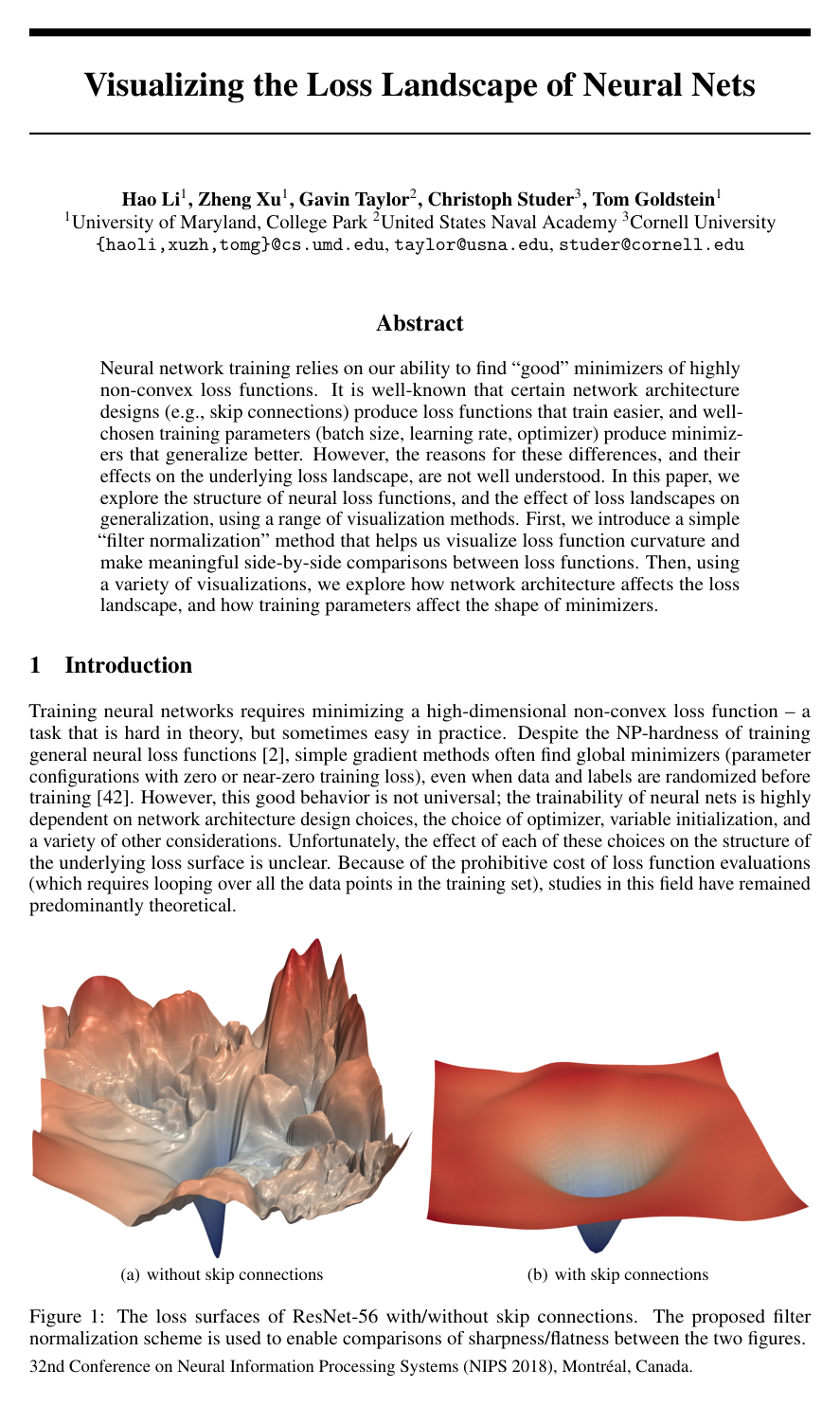
The analysis produced four primary findings. First, as network depth increases in architectures without shortcut connections, the loss surface undergoes an abrupt transition from benign, nearly convex geometry to extreme chaos; for example, removing skip connections caused the test error of a 110-layer network to degrade from 5.79% to 16.44%. Second, skip connections directly prevent this chaotic transition, preserving wide, well-behaved loss basins across deep models. Third, increasing layer width similarly flattens the landscape and eliminates chaotic behavior, with wider models achieving superior generalization. Fourth, true loss landscape flatness consistently correlates with superior generalization performance, and optimization paths are highly structured, with between 40% and 90% of training trajectory variation captured in just two dimensions.

These findings have direct operational and strategic implications for machine learning deployment. Designing deep models without architectural stabilizers like skip connections introduces severe risks of training failure, volatile gradient behavior, and poor accuracy, driving up computational costs. Conversely, incorporating skip connections and adequate layer width ensures reliable training, reduces sensitivity to initial parameter choices, and delivers more robust predictive models for high-stakes business environments.

Organizations developing deep learning systems should mandate architectural features such as residual shortcut connections or wider layer designs for deep networks. When diagnosing model performance or evaluating training dynamics, engineering teams should adopt filter-normalized loss visualization rather than unnormalized or layer-normalized alternatives. Future work should extend these visualization protocols to larger-scale datasets and emerging non-convolutional architectures to validate broader applicability.

Confidence in these conclusions is high, backed by repeated empirical trials, mathematical curvature validations, and open-source verification. A known limitation is that two-dimensional projections inherently compress high-dimensional spaces; however, explicit eigenvalue calculations confirm that the visual convexity accurately reflects genuine high-dimensional stability rather than projection artifacts.

Cornell University United States Naval Academy University of Maryland architecture designs network architecture neural networks Loss Neural Figure

arXiv: 1712.09913 tomgoldstein/loss-landscape

Paper: Understanding deep learning requires rethinking generalization, Chiyuan Zhang et al. (2017). This foundational paper reveals the puzzling generalization properties of overparameterized networks that the source paper investigates through loss landscape visualization.
Paper: On Large-Batch Training for Deep Learning: Generalization Gap and Sharp Minima, Nitish Shirish Keskar et al. (2016). This work directly connects large-batch training deficiencies to sharp minimizers, providing crucial context for the source paper's study of training parameter effects on landscape geometry.
Paper: Identity Mappings in Deep Residual Networks, Kaiming He et al. (2016). This study demonstrates how skip connections ease optimization and alter network depth, serving as a direct prerequisite for the source paper's architectural loss landscape comparisons.

Paper: Neural Tangent Kernel: Convergence and Generalization in Neural Networks, Arthur Jacot et al. (2018). Building upon the source paper's empirical interest in loss landscapes, this work provides a rigorous theoretical characterization of gradient descent dynamics and convergence in the infinite-width limit.
Paper: On the Spectral Bias of Neural Networks, Nasim Rahaman et al. (2019). Extending the source's exploration of non-convex loss functions, this paper investigates the implicit spectral biases that govern how neural networks navigate their loss landscapes during training.

Cover for Visualizing the Loss Landscape of Neural Nets

Abstract

Neural network training relies on our ability to find "good" minimizers of highly non-convex loss functions. It is well-known that certain network architecture designs (e.g., skip connections) produce loss functions that train easier, and well-chosen training parameters (batch size, learning rate, optimizer) produce minimizers that generalize better. However, the reasons for these differences, and their effects on the underlying loss landscape, are not well understood. In this paper, we explore the structure of neural loss functions, and the effect of loss landscapes on generalization, using a range of visualization methods. First, we introduce a simple "filter normalization" method that helps us visualize loss function curvature and make meaningful side-by-side comparisons between loss functions. Then, using a variety of visualizations, we explore how network architecture affects the loss landscape, and how training parameters affect the shape of minimizers.

Topics

architecture designs network architecture neural networks visualization tools

Keywords

Loss Neural Figure Training Accuracy Plots Networks SGD Normalization Network

1 Introduction
1.1 Contributions
2 Theoretical Background
3 The Basics of Loss Function Visualization
4 Proposed Visualization: Filter-Wise Normalization
5 The Sharp vs Flat Dilemma
6 What Makes Neural Networks Trainable? Insights on the (Non)Convexity Structure of Loss Surfaces
7 Visualizing Optimization Paths
7.1 Why Random Directions Fail: Low-Dimensional Optimization Trajectories
7.2 Effective Trajectory Plotting using PCA Directions
8 Conclusion
References
A Comparison of Loss Surfaces
A.1 The Change of Weights Norm during Training
A.2 Comparision of Normalization Methods
A.3 Small-Batch vs Large-Batch for ResNet-56
A.4 Repeatability of the Loss Surface Visualization
A.5 Implementation Details
A.6 Training Curves for VGG-9 and ResNets

Knowls

Knowl 1 — Filter-Wise Direction Normalization for Loss Surface Visualization
model/method
Neural networks with rectified linear unit (ReLU) activations and Batch Normalization exhibit scale invariance: multiplying the weights of one layer by a scalar $c > 0$ and dividing the subsequent layer by $c$ leaves the network's predictive function unchanged, while altering the parameter norms. Under unnormalized perturbations, a model with large parameter norms appears artificially flat and insensitive to weight changes, whereas an equivalent model with small parameter norms appears artificially sharp.

To remove scaling artifacts and enable meaningful side-by-side comparisons of loss surface geometry across different architectures, optimizers, and regularization settings, filter-wise normalization rescales each filter of a random direction vector $d \in \mathbb{R}^D$ to match the Frobenius norm of the corresponding parameter filter in the weight vector $\theta \in \mathbb{R}^D$ : $d_{i,j} \leftarrow \frac{d_{i,j}}{\|d_{i,j}\|_F} \|\theta_{i,j}\|_F$ where $\theta_{i,j}$ is the weight tensor representing the $j$ -th filter in the $i$ -th layer of $\theta$ , $d_{i,j}$ is the corresponding slice of $d$ , and $\|\cdot\|_F$ denotes the Frobenius norm. For fully connected layers, each neuron's incoming weight vector is treated as a filter (equivalent to a $1 \times 1$ convolutional filter). Batch normalization parameters (e.g., running mean and variance) are kept unperturbed and held constant during evaluation.
Knowl 2 — Two-Dimensional Loss Surface Profiling via Filter-Normalized Random Coordinates
model/method
Let $\theta^* \in \mathbb{R}^D$ denote a neural network parameter configuration (such as a local minimizer obtained at the end of training), and let $L(\theta)$ denote the empirical loss function over a dataset of $m$ input-label pairs $\{(x_i, y_i)\}_{i=1}^m$ : $L(\theta) = \frac{1}{m} \sum_{i=1}^m \ell(x_i, y_i; \theta)$ To visualize the two-dimensional loss landscape slice centered at $\theta^*$ , the loss is evaluated across a two-dimensional grid of coordinate offsets $(\alpha, \beta) \in \mathbb{R}^2$ : $f(\alpha, \beta) = L(\theta^* + \alpha \delta + \beta \eta)$ where $\delta, \eta \in \mathbb{R}^D$ are direction vectors independently sampled from a standard Gaussian distribution $\mathcal{N}(0, I_D)$ and normalized filter-by-filter with respect to $\theta^*$ : $\delta_{i,j} \leftarrow \frac{\delta_{i,j}}{\|\delta_{i,j}\|_F} \|\theta^*_{i,j}\|_F, \quad \eta_{i,j} \leftarrow \frac{\eta_{i,j}}{\|\eta_{i,j}\|_F} \|\theta^*_{i,j}\|_F$ for every filter $j$ in layer $i$ . Evaluating $f(\alpha, \beta)$ over a dense grid produces contour and surface plots that reflect the scale-invariant curvature and non-convexity surrounding $\theta^*$ .
Knowl 3 — Resolution of the Sharpness-Generalization Contradiction under Weight Decay
empirical result
Evaluating 1D linear interpolations $f(\alpha) = L((1-\alpha)\theta_s + \alpha \theta_l)$ between small-batch (batch size 128, denoted $\theta_s$ ) and large-batch (batch size 8192, denoted $\theta_l$ ) minimizers produces contradictory sharpness assessments depending on weight decay:
1. Without weight decay ( $WD = 0$ ), the small-batch minimizer $\theta_s$ has larger parameter norms than $\theta_l$ , causing $\theta_s$ to appear flatter and $\theta_l$ to appear sharper.
2. With weight decay ( $WD = 5 \times 10^{-4}$ ), small-batch training performs more parameter updates per epoch, causing weight decay penalties to shrink the norm of $\theta_s$ significantly below that of $\theta_l$ . Consequently, unnormalized linear interpolation makes $\theta_l$ appear flatter than $\theta_s$ , despite $\theta_s$ achieving better test performance (6.00% vs. 10.19% test error on CIFAR-10 for VGG-9).
When filter-wise normalization is applied independently around each minimizer, the parameter scaling artifact is eliminated: small-batch minimizers consistently display wider, flatter contours than large-batch minimizers across both SGD and Adam optimizers, establishing a consistent correlation between visual flatness and lower generalization error.
Knowl 4 — Depth-Induced Transition from Convexity to Chaotic Loss Surfaces in Plain Networks
empirical result
In feedforward convolutional neural networks lacking shortcut/skip connections (plain networks constructed by removing residual connections from ResNet architectures), increasing network depth causes the loss landscape to transition from a benign, nearly convex surface to a highly chaotic, rugged surface:
- At 20 layers (ResNet-20-noshort), the loss landscape is dominated by a large, nearly convex central basin with smooth, well-conditioned contours around the minimizer.
- At 56 layers (ResNet-56-noshort), the loss landscape exhibits dramatic non-convexities, ill-conditioned eccentric contours, and wide plateau regions where gradient vectors point away from the central minimum.
- At 110 layers (ResNet-110-noshort), the loss surface becomes extremely steep and chaotic in all directions, causing CIFAR-10 test error to deteriorate to 16.44% (compared to 5.79% for ResNet-110 with skip connections).
- At 156 layers without skip connections, SGD fails to train entirely due to gradient shattering, as random initialization strategies place initial weights on chaotic plateaus with uninformative gradients.
Knowl 5 — Prevention of Loss Surface Chaos by Shortcut Connections
empirical result
Incorporating identity shortcut connections (as in ResNets and DenseNets) prevents the explosion of non-convexity that occurs as depth increases in plain feedforward networks:
- In ResNet architectures (ResNet-20, ResNet-56, ResNet-110), the loss landscape retains a smooth, wide, nearly convex basin around the minimizer regardless of network depth.
- The width and shape of the 0.1-level loss contour are virtually identical across 20-layer and 110-layer ResNet models.
- In DenseNet-121, the loss surface is completely dominated by a smooth, nearly convex basin with no observable non-convexity.
Residual connections preserve deep and wide basins of attraction, allowing standard random initializations (such as Glorot/Xavier initialization) to land within the convex basin where gradient directions consistently lead toward the global minimizer.
Knowl 6 — Loss Landscape Smoothing and Widening through Increased Network Width
empirical result
Increasing the number of convolutional filters per layer (network width) significantly widens minimizers and smooths the loss landscape in both residual and non-residual networks:
- In Wide-ResNet-56 architectures where the number of filters per layer is scaled by a width factor $k \in \{1, 2, 4, 8\}$ , higher values of $k$ systematically broaden the central minimizer and eliminate chaotic landscape features.
- For residual networks on CIFAR-10, increasing width yields monotonic improvements in test error: $k=1$ achieves 5.89%, $k=2$ achieves 5.07%, $k=4$ achieves 4.34%, and $k=8$ achieves 3.93%.
- For non-residual networks (ResNet-56-noshort), increasing width from $k=1$ to $k=8$ suppresses chaotic non-convexities and reduces test error from 13.31% to 8.70%.
Knowl 7 — Hessian Spectrum and Principle Curvature Validity in 2D Projections
theoretical result
For a loss function $L: \mathbb{R}^D \to \mathbb{R}$ , the principle curvatures computed on a 2D slice spanned by random Gaussian directions are weighted averages of the true eigenvalues of the high-dimensional Hessian $\nabla^2 L(\theta)$ , where the weights are independent Chi-square distributed random variables.

This relationship implies:
1. If negative curvature (non-convexity) is present in the 2D projected plot, the high-dimensional Hessian must possess negative eigenvalues.
2. Apparent convexity in a 2D slice indicates that positive curvatures dominate in expectation (i.e., the mean curvature is positive).
Computing the extreme Hessian eigenvalues $\lambda_{\min}$ and $\lambda_{\max}$ via an implicitly restarted Lanczos method reveals that visually convex regions (such as in ResNet-56 and DenseNet-121) have $|\lambda_{\min} / \lambda_{\max}| < 0.01$ over large areas (negative eigenvalues are less than 1% of the magnitude of positive eigenvalues), whereas chaotic loss surfaces (such as ResNet-56-noshort) contain large negative eigenvalues with $|\lambda_{\min} / \lambda_{\max}| > 0.4$ .
Knowl 8 — PCA-Based Optimization Trajectory Projection Algorithm
algorithm
Random direction vectors in high dimension $D$ are nearly orthogonal with high probability (the expected cosine similarity between two random Gaussian vectors in $\mathbb{R}^D$ is approximately $\sqrt{2 / (\pi D)}$ ), causing projections of optimization paths onto random directions to fail to capture trajectory variance. Applying Principal Component Analysis (PCA) to the sequence of parameter checkpoints extracts the low-dimensional subspace capturing the descent path.
Input: Model parameter iterates across $n$ epochs $\theta_0, \theta_1, \dots, \theta_n \in \mathbb{R}^D$ , dataset loss function $L(\theta)$
Output: 2D trajectory coordinates $(x_i, y_i)_{i=0}^n$ and 2D loss surface function $f(\alpha, \beta)$
Construct the parameter displacement matrix $M \in \mathbb{R}^{n \times D}$ relative to the final solution $\theta_n$ :
     $M = [(\theta_0 - \theta_n)^T; (\theta_1 - \theta_n)^T; \dots; (\theta_{n-1} - \theta_n)^T]$
Compute the top two principal component directions $v_1, v_2 \in \mathbb{R}^D$ of $M$ via Singular Value Decomposition
Apply filter-wise normalization to direction vectors $v_1$ and $v_2$ relative to $\theta_n$ :
     $e_{1, (j,k)} \leftarrow \frac{v_{1, (j,k)}}{\|v_{1, (j,k)}\|_F} \|\theta_{n, (j,k)}\|_F$
     $e_{2, (j,k)} \leftarrow \frac{v_{2, (j,k)}}{\|v_{2, (j,k)}\|_F} \|\theta_{n, (j,k)}\|_F$
    for each filter $k$ in layer $j$
Project each parameter iterate $\theta_i$ for $i \in \{0, \dots, n\}$ onto the principal directions:
     $x_i \leftarrow \langle \theta_i - \theta_n, v_1 \rangle$
     $y_i \leftarrow \langle \theta_i - \theta_n, v_2 \rangle$
Define the 2D loss evaluation function over coordinate grid $(\alpha, \beta)$ :
     $f(\alpha, \beta) = L(\theta_n + \alpha e_1 + \beta e_2)$
return $(x_i, y_i)_{i=0}^n$ , $f(\alpha, \beta)$
Knowl 9 — Low-Dimensional Concentration of SGD and Adam Optimization Trajectories
empirical result
When PCA is applied to the trajectory of parameter iterates $\theta_0, \dots, \theta_n$ during training on CIFAR-10 with SGD (with momentum) or Adam across small (128) and large (8192) batch sizes:
- The top 2 principal component directions account for $40\%$ to $90\%$ of the total variance in the optimization path.
- In early training epochs, optimization trajectories move perpendicular to the loss contours along deterministic gradient directions.
- In later training epochs (particularly under small batch sizes and non-zero weight decay), the trajectory exhibits stochastic orbiting around the minimizer until the learning rate is decreased, at which point the effective noise drops and the trajectory falls into the nearest local minimizer.

Knowl 10 — CIFAR-10 Benchmark Comparison for Plain versus Residual Networks

data/table

The table below lists the training loss, training error (%), and test error (%) for CIFAR-10 classification across ResNet models (with skip connections) and ResNet-noshort models (without skip connections) at depths 20, 56, and 110. Models are trained with SGD with Nesterov momentum, batch size 128, and weight decay $5 \times 10^{-4}$ for 300 epochs, with learning rate decayed by a factor of 10 at epochs 150, 225, and 275.

Model	Initial LR	Training Loss	Training Error (%)	Test Error (%)
ResNet-20	0.1	0.017	0.286	7.37
ResNet-20-noshort	0.1	0.025	0.560	8.18
ResNet-56	0.1	0.004	0.052	5.89
ResNet-56-noshort	0.1	0.192	6.494	13.31
ResNet-56-noshort	0.01	0.024	0.704	10.83
ResNet-110	0.1	0.002	0.042	5.79
ResNet-110-noshort	0.01	0.258	8.732	16.44

These results show that at 20 layers, removing shortcut connections causes only a minor test error increase (from 7.37% to 8.18%). At 56 and 110 layers, plain networks without skip connections fail to converge at the default learning rate of 0.1 and suffer substantial test error degradation even when the initial learning rate is tuned to 0.01 (10.83% vs. 5.89% for 56 layers, and 16.44% vs. 5.79% for 110 layers).

Coverage note — None was omitted; all main contributions, including the filter normalization method, architectural effects (depth, width, skip connections), sharp vs. flat dilemma resolution, Hessian spectrum analysis, trajectory visualization, and benchmark data tables, are covered.

References

1.David Balduzzi, Marcus Frean, Lennox Leary, JP Lewis, Kurt Wan-Duo Ma, and Brian McWilliams. The shattered gradients problem: If resnets are the answer, then what is the question? In ICML, 2017.
2.Avrim Blum and Ronald L Rivest. Training a 3-node neural network is np-complete. In NIPS, 1989.
3.Pratik Chaudhari, Anna Choromanska, Stefano Soatto, and Yann LeCun. Entropy-sgd: Biasing gradient descent into wide valleys. In ICLR, 2017.
4.Anna Choromanska, Mikael Henaff, Michael Mathieu, Gérard Ben Arous, and Yann LeCun. The loss surfaces of multilayer networks. In AISTATS, 2015.
5.Yann N Dauphin, Razvan Pascanu, Caglar Gulcehre, Kyunghyun Cho, Surya Ganguli, and Yoshua Bengio. Identifying and attacking the saddle point problem in high-dimensional non-convex optimization. In NIPS, 2014.
6.Soham De, Abhay Yadav, David Jacobs, and Tom Goldstein. Automated inference with adaptive batches. In AISTATS, 2017.
7.Laurent Dinh, Razvan Pascanu, Samy Bengio, and Yoshua Bengio. Sharp minima can generalize for deep nets. In ICML, 2017.
8.Gintare Karolina Dziugaite and Daniel M Roy. Computing nonvacuous generalization bounds for deep (stochastic) neural networks with many more parameters than training data. In UAI, 2017.
9.C Daniel Freeman and Joan Bruna. Topology and geometry of half-rectified network optimization. In ICLR, 2017.
10.Marcus Gallagher and Tom Downs. Visualization of learning in multilayer perceptron networks using principal component analysis. IEEE Transactions on Systems, Man, and Cybernetics, Part B (Cybernetics), 33(1):28–34, 2003.
11.Xavier Glorot and Yoshua Bengio. Understanding the difficulty of training deep feedforward neural networks. In AISTATS, 2010.
12.Tom Goldstein and Christoph Studer. Phasemax: Convex phase retrieval via basis pursuit. arXiv preprint arXiv:1610.07531, 2016.
13.Ian J Goodfellow, Oriol Vinyals, and Andrew M Saxe. Qualitatively characterizing neural network optimization problems. In ICLR, 2015.
14.Priya Goyal, Piotr Dollár, Ross Girshick, Pieter Noordhuis, Lukasz Wesolowski, Aapo Kyrola, Andrew Tulloch, Yangqing Jia, and Kaiming He. Accurate, large minibatch sgd: Training imagenet in 1 hour. arXiv preprint arXiv:1706.02677, 2017.
15.Benjamin D Haeffele and René Vidal. Global optimality in neural network training. In CVPR, 2017.
16.Moritz Hardt and Tengyu Ma. Identity matters in deep learning. In ICLR, 2017.
17.Kaiming He, Xiangyu Zhang, Shaoqing Ren, and Jian Sun. Deep Residual Learning for Image Recognition. In CVPR, 2016.
18.Sepp Hochreiter and Jürgen Schmidhuber. Flat minima. Neural Computation, 9(1):1–42, 1997.
19.Elad Hoffer, Itay Hubara, and Daniel Soudry. Train longer, generalize better: closing the generalization gap in large batch training of neural networks. NIPS, 2017.
20.Gao Huang, Zhuang Liu, Kilian Q Weinberger, and Laurens van der Maaten. Densely connected convolutional networks. In CVPR, 2017.
21.Daniel Jiwoong Im, Michael Tao, and Kristin Branson. An empirical analysis of deep network loss surfaces. arXiv preprint arXiv:1612.04010, 2016.
22.Sergey Ioffe and Christian Szegedy. Batch Normalization: Accelerating Deep Network Training by Reducing Internal Covariate Shift. In ICML, 2015.
23.Kenji Kawaguchi, Leslie Pack Kaelbling, and Yoshua Bengio. Generalization in deep learning. arXiv preprint arXiv:1710.05468, 2017.
24.Nitish Shirish Keskar, Dheevatsa Mudigere, Jorge Nocedal, Mikhail Smelyanskiy, and Ping Tak Peter Tang. On large-batch training for deep learning: Generalization gap and sharp minima. In ICLR, 2017.
25.Anders Krogh and John A Hertz. A simple weight decay can improve generalization. In NIPS, 1992.
26.Yuanzhi Li and Yang Yuan. Convergence analysis of two-layer neural networks with relu activation. arXiv preprint arXiv:1705.09886, 2017.
27.Qianli Liao and Tomaso Poggio. Theory of deep learning ii: Landscape of the empirical risk in deep learning. arXiv preprint arXiv:1703.09833, 2017.
28.Zachary C Lipton. Stuck in a what? adventures in weight space. In ICLR Workshop, 2016.
29.Eliana Lorch. Visualizing deep network training trajectories with pca. In ICML Workshop on Visualization for Deep Learning, 2016.
30.Behnam Neyshabur, Srinadh Bhojanapalli, David McAllester, and Nati Srebro. Exploring generalization in deep learning. In NIPS, 2017.
31.Quynh Nguyen and Matthias Hein. The loss surface of deep and wide neural networks. In ICML, 2017.
32.Itay Safran and Ohad Shamir. On the quality of the initial basin in overspecified neural networks. In ICML, 2016.
33.Karen Simonyan and Andrew Zisserman. Very Deep Convolutional Networks for Large-Scale Image Recognition. In ICLR, 2015.
34.Leslie N Smith and Nicholay Topin. Exploring loss function topology with cyclical learning rates. arXiv preprint arXiv:1702.04283, 2017.
35.Mahdi Soltanolkotabi, Adel Javanmard, and Jason D Lee. Theoretical insights into the optimization landscape of over-parameterized shallow neural networks. arXiv preprint arXiv:1707.04926, 2017.
36.Daniel Soudry and Elad Hoffer. Exponentially vanishing sub-optimal local minima in multilayer neural networks. arXiv preprint arXiv:1702.05777, 2017.
37.Grzegorz Swirszcz, Wojciech Marian Czarnecki, and Razvan Pascanu. Local minima in training of deep networks. arXiv preprint arXiv:1611.06310, 2016.
38.Yuandong Tian. An analytical formula of population gradient for two-layered relu network and its applications in convergence and critical point analysis. In ICML, 2017.
39.Bo Xie, Yingyu Liang, and Le Song. Diverse neural network learns true target functions. In AISTATS, 2017.
40.Chulhee Yun, Suvrit Sra, and Ali Jadbabaie. Global optimality conditions for deep neural networks. In ICLR, 2017.
41.Sergey Zagoruyko and Nikos Komodakis. Wide residual networks. In BMVC, 2016.
42.Chiyuan Zhang, Samy Bengio, Moritz Hardt, Benjamin Recht, and Oriol Vinyals. Understanding deep learning requires rethinking generalization. In ICLR, 2017.

Citation

MLA

Li, H., et al. “Visualizing the Loss Landscape of Neural Nets”. arXiv, 2017, https://doi.org/10.48550/arxiv.1712.09913.

APA

Li, H., Xu, Z., Taylor, G., Studer, C., & Goldstein, T. (2017). Visualizing the Loss Landscape of Neural Nets. arXiv. https://doi.org/10.48550/arxiv.1712.09913

Chicago

Li, H., Z. Xu, G. Taylor, C. Studer, and T. Goldstein. 2017. “Visualizing the Loss Landscape of Neural Nets”. Preprint, ArXiv. https://doi.org/10.48550/arxiv.1712.09913.

Harvard

Li, H. et al. (2017) “Visualizing the Loss Landscape of Neural Nets”. arXiv. Available at: https://doi.org/10.48550/arxiv.1712.09913.

Vancouver

1. Li H, Xu Z, Taylor G, Studer C, Goldstein T (2017) Visualizing the Loss Landscape of Neural Nets. https://doi.org/10.48550/arxiv.1712.09913

BibTeX

@misc{https://doi.org/10.48550/arxiv.1712.09913,
  doi = {10.48550/ARXIV.1712.09913},
  url = {https://arxiv.org/abs/1712.09913},
  author = {Li, Hao and Xu, Zheng and Taylor, Gavin and Studer, Christoph and Goldstein, Tom},
  keywords = {Machine Learning (cs.LG), Computer Vision and Pattern Recognition (cs.CV), Machine Learning (stat.ML), FOS: Computer and information sciences, FOS: Computer and information sciences},
  title = {Visualizing the Loss Landscape of Neural Nets},
  publisher = {arXiv},
  year = {2017},
  copyright = {arXiv.org perpetual, non-exclusive license}
}

Metadata:DOI registry

Source Code

This paper has an official code repository available. Click below to access the source code.

View Repository

Access the Paper

This paper is available from its original source. Click below to access the PDF.

Open PDF

License: Authors

Visualizing the Loss Landscape of Neural Nets

Abstract

Topics

Keywords

Table of Contents

Knowls

Knowl 1 — Filter-Wise Direction Normalization for Loss Surface Visualization

Knowl 2 — Two-Dimensional Loss Surface Profiling via Filter-Normalized Random Coordinates

Knowl 3 — Resolution of the Sharpness-Generalization Contradiction under Weight Decay

Knowl 4 — Depth-Induced Transition from Convexity to Chaotic Loss Surfaces in Plain Networks

Knowl 5 — Prevention of Loss Surface Chaos by Shortcut Connections

Knowl 6 — Loss Landscape Smoothing and Widening through Increased Network Width

Knowl 7 — Hessian Spectrum and Principle Curvature Validity in 2D Projections