On Large-Batch Training for Deep Learning: Generalization Gap and Sharp Minima

Nitish Shirish KeskarDheevatsa MudigereJorge NocedalMikhail SmelyanskiyPing Tak Peter Tang

article2016ICLR3,587 citations

Demonstrates that the generalization drop in large-batch deep learning training stems from convergence to sharp minimizers, contrasting this with small-batch methods that inherently reach flat minima through gradient noise.

Listen

Large-batch training of deep neural networks produces models that generalize noticeably worse than those trained with conventional small batches, even when both reach comparable training accuracy. This gap limits the use of large batches to accelerate parallel training on many processors, an increasingly attractive option as data sets and models grow. The work set out to identify the underlying cause through controlled numerical experiments rather than theory alone.

Researchers trained six representative networkstwo fully connected and four convolutionalon MNIST, TIMIT, CIFAR-10, and CIFAR-100. They compared the ADAM optimizer run with a fixed small batch of 256 examples against a large batch equal to 10 percent of the training set. Solutions were characterized with one-dimensional parametric slices between small-batch and large-batch minima and with a computationally feasible sensitivity metric that quantifies how rapidly the loss rises in a small neighborhood of each solution.

The experiments show that large-batch runs consistently converge to sharp minimizers whose loss surfaces rise steeply along a modest number of directions, whereas small-batch runs reach flat minimizers. The sharpness metric differs by one to two orders of magnitude between the two regimes, and the testing-accuracy gap reaches several percentage points. The difference is not explained by overfitting; early-stopping does not close it. Noise inherent in small-batch gradient estimates appears to eject iterates from basins of sharp minima, an effect that disappears once the batch exceeds a network-specific threshold.

These results imply that any attempt to scale deep-learning training by simply enlarging the batch will encounter a generalization penalty unless the optimizer is modified to avoid sharp regions. Because training time can drop dramatically with larger batches when parallelism is high, closing the gap would materially shorten development cycles for large models.

Simple remedies such as data augmentation, conservative (proximal) updates, and adversarial training narrow the accuracy difference modestly but still produce relatively sharp solutions. Dynamic batch-size schedules that begin small and grow, or warm-starting a large-batch run from a short small-batch phase, appear more promising and warrant further study. The main limitations are that the sharpness measure is a practical proxy rather than an exact eigenvalue computation and that the networks and data sets, while representative, do not exhaust modern architectures.

  • Paper: Optimization Methods for Large-Scale Machine Learning, Léon Bottou et al. (2016). Reading this foundational survey on stochastic gradient methods and large-scale optimization clarifies the computational and theoretical trade-offs that motivate the generalization gap in large-batch training.
  • Paper: An overview of gradient descent optimization algorithms, Sebastian Ruder (2016). Understanding the mechanics and mini-batch dynamics of gradient descent optimization algorithms provides necessary context for analyzing how batch size influences convergence behavior.
  • Paper: Accurate, Large Minibatch SGD: Training ImageNet in 1 Hour, Priya Goyal et al. (2017). This follow-up work extends the source study by demonstrating that large-minibatch SGD can successfully scale to massive batch sizes of 8,192 images without a generalization drop when paired with learning rate warmups and linear scaling.
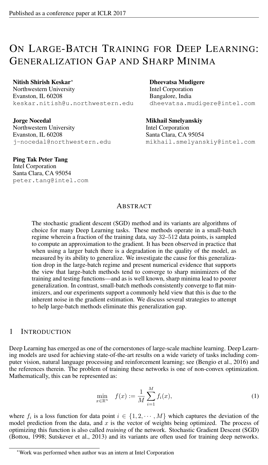
Cover for On Large-Batch Training for Deep Learning: Generalization Gap and Sharp Minima

Abstract

The stochastic gradient descent (SGD) method and its variants are algorithms of choice for many Deep Learning tasks. These methods operate in a small-batch regime wherein a fraction of the training data, say 3232-512512 data points, is sampled to compute an approximation to the gradient. It has been observed in practice that when using a larger batch there is a degradation in the quality of the model, as measured by its ability to generalize. We investigate the cause for this generalization drop in the large-batch regime and present numerical evidence that supports the view that large-batch methods tend to converge to sharp minimizers of the training and testing functions - and as is well known, sharp minima lead to poorer generalization. In contrast, small-batch methods consistently converge to flat minimizers, and our experiments support a commonly held view that this is due to the inherent noise in the gradient estimation. We discuss several strategies to attempt to help large-batch methods eliminate this generalization gap.

Table of Contents

  • 1 INTRODUCTION
  • 1.1 NOTATION
  • 2 DRAWBACKS OF LARGE-BATCH METHODS
  • 2.1 OUR MAIN OBSERVATION
  • 2.2 NUMERICAL EXPERIMENTS
  • 2.2.1 PARAMETRIC PLOTS
  • 2.2.2 SHARPNESS OF MINIMA
  • 3 SUCCESS OF SMALL-BATCH METHODS
  • 4 DISCUSSION AND CONCLUSION
  • A DETAILS ABOUT DATA SETS
  • B ARCHITECTURE OF NETWORKS
  • B.1 NETWORK F1F_1
  • B.2 NETWORK F2F_2
  • B.3 NETWORKS C1C_1 AND C3C_3
  • B.4 NETWORKS C2C_2 AND C4C_4
  • C PERFORMANCE MODEL
  • D CURVILINEAR PARAMETRIC PLOTS
  • E ATTEMPTS TO IMPROVE LB METHODS
  • E.1 DATA AUGMENTATION
  • E.2 CONSERVATIVE TRAINING
  • E.3 ROBUST TRAINING

Knowls

  1. Knowl 1 — Generalization Gap in Large-Batch Deep Learning

    empirical result

    When training deep neural networks, using large mini-batches (e.g., 10%10\% of the training set size) leads to a noticeable decline in generalization performance (testing accuracy) compared to small mini-batches (e.g., batch size 256), even though both regimes achieve near-identical training loss and accuracy.

    The table below presents the training and testing accuracies obtained using the ADAM optimizer with small batches (SB\text{SB}, batch size 256) and large batches (LB\text{LB}, batch size equal to 10%10\% of the training set) across six multi-class classification networks: fully connected architectures on MNIST (F1F_1) and TIMIT (F2F_2), shallow convolutional architectures on CIFAR-10 (C1C_1) and CIFAR-100 (C3C_3), and deep convolutional architectures on CIFAR-10 (C2C_2) and CIFAR-100 (C4C_4). Results report the mean and standard deviation over 5 independent runs from random initializations, trained until the training loss ceased to improve:

    Network SB Training Acc. LB Training Acc. SB Testing Acc. LB Testing Acc.
    F1F_1 (MNIST FC) 99.66%±0.05%99.66\% \pm 0.05\% 99.92%±0.01%99.92\% \pm 0.01\% 98.03%±0.07%98.03\% \pm 0.07\% 97.81%±0.07%97.81\% \pm 0.07\%
    F2F_2 (TIMIT FC) 99.99%±0.03%99.99\% \pm 0.03\% 98.35%±2.08%98.35\% \pm 2.08\% 64.02%±0.20%64.02\% \pm 0.20\% 59.45%±1.05%59.45\% \pm 1.05\%
    C1C_1 (CIFAR-10 Shallow CNN) 99.89%±0.02%99.89\% \pm 0.02\% 99.66%±0.20%99.66\% \pm 0.20\% 80.04%±0.12%80.04\% \pm 0.12\% 77.26%±0.42%77.26\% \pm 0.42\%
    C2C_2 (CIFAR-10 Deep CNN) 99.99%±0.04%99.99\% \pm 0.04\% 99.99%±0.01%99.99\% \pm 0.01\% 89.24%±0.12%89.24\% \pm 0.12\% 87.26%±0.07%87.26\% \pm 0.07\%
    C3C_3 (CIFAR-100 Shallow CNN) 99.56%±0.44%99.56\% \pm 0.44\% 99.88%±0.30%99.88\% \pm 0.30\% 49.58%±0.39%49.58\% \pm 0.39\% 46.45%±0.43%46.45\% \pm 0.43\%
    C4C_4 (CIFAR-100 Deep CNN) 99.10%±1.23%99.10\% \pm 1.23\% 99.57%±1.84%99.57\% \pm 1.84\% 63.08%±0.50%63.08\% \pm 0.50\% 57.81%±0.17%57.81\% \pm 0.17\%

    The generalization gap (difference between SB\text{SB} and LB\text{LB} testing accuracy) ranges from 0.2%\approx 0.2\% up to over 5%5\%. This degradation is not caused by conventional statistical overfitting or over-training, as the testing accuracy for LB\text{LB} does not peak and decay over epochs, but rather plateaus at an inferior value.

  2. Knowl 2 — $(C_\epsilon, A)$-Sharpness Metric for Neural Network Minima

    definition

    To quantify the sensitivity and flatness of a loss function f:RnRf: \mathbb{R}^n \to \mathbb{R} at a local minimizer xRnx \in \mathbb{R}^n, the (Cϵ,A)(C_\epsilon, A)-sharpness metric measures the maximum relative increase of ff in a constrained box defined over the full parameter space or projected onto a lower-dimensional subspace.

    Given xRnx \in \mathbb{R}^n, a box size parameter ϵ>0\epsilon > 0, and a projection matrix ARn×pA \in \mathbb{R}^{n \times p} (where pnp \le n defines the subspace dimension, and A=InA = I_n for full-space evaluation), the constraint set CϵRpC_\epsilon \subset \mathbb{R}^p is defined to ensure invariance to problem dimension and parameter scale: Cϵ={zRp:ϵ((A+x)i+1)ziϵ((A+x)i+1),  i{1,2,,p}},C_\epsilon = \left\{ z \in \mathbb{R}^p : -\epsilon \left(|(A^+ x)_i| + 1\right) \le z_i \le \epsilon \left(|(A^+ x)_i| + 1\right), \; \forall i \in \{1, 2, \dots, p\} \right\}, where A+A^+ denotes the Moore-Penrose pseudo-inverse of AA.

    The (Cϵ,A)(C_\epsilon, A)-sharpness of ff at xx is defined as: ϕx,f(ϵ,A)=(maxyCϵf(x+Ay))f(x)1+f(x)×100.\phi_{x,f}(\epsilon, A) = \frac{\left(\max_{y \in C_\epsilon} f(x + A y)\right) - f(x)}{1 + f(x)} \times 100.

    When ϵ\epsilon is sufficiently small and A=InA = I_n, ϕx,f(ϵ,In)\phi_{x,f}(\epsilon, I_n) relates to the largest eigenvalue of the Hessian 2f(x)\nabla^2 f(x). When ARn×pA \in \mathbb{R}^{n \times p} is a randomly sampled matrix, it approximates the largest Ritz value of 2f(x)\nabla^2 f(x) projected onto the column space of AA. In practice, the inner maximization over CϵC_\epsilon is solved inexactly using 10 iterations of L-BFGS-B.

  3. Knowl 3 — Sharpness Disparity Between Small-Batch and Large-Batch Minima

    empirical result

    Minimizers located by large-batch (LB\text{LB}) methods exhibit (Cϵ,A)(C_\epsilon, A)-sharpness values that are 1 to 2 orders of magnitude higher than those found by small-batch (SB\text{SB}) methods, both across the full parameter space (A=InA = I_n) and across random 100-dimensional subspaces (ARn×100A \in \mathbb{R}^{n \times 100}).

    The tables below report the mean and standard deviation of (Cϵ,A)(C_\epsilon, A)-sharpness across 5 runs for small batches (SB\text{SB}, batch size 256) and large batches (LB\text{LB}, batch size 10%10\% of training data) at perturbation scales ϵ=103\epsilon = 10^{-3} and ϵ=5104\epsilon = 5 \cdot 10^{-4}:

    Full space (A=InA = I_n):

    ϵ=103\epsilon = 10^{-3} ϵ=5104\epsilon = 5 \cdot 10^{-4}
    Network SB LB SB LB
    F1F_1 (MNIST FC) 1.23±0.831.23 \pm 0.83 205.14±69.52205.14 \pm 69.52 0.61±0.270.61 \pm 0.27 42.90±17.1442.90 \pm 17.14
    F2F_2 (TIMIT FC) 1.39±0.021.39 \pm 0.02 310.64±38.46310.64 \pm 38.46 0.90±0.050.90 \pm 0.05 93.15±6.8193.15 \pm 6.81
    C1C_1 (CIFAR-10 Shallow CNN) 28.58±3.1328.58 \pm 3.13 707.23±43.04707.23 \pm 43.04 7.08±0.887.08 \pm 0.88 227.31±23.23227.31 \pm 23.23
    C2C_2 (CIFAR-10 Deep CNN) 8.68±1.328.68 \pm 1.32 925.32±38.29925.32 \pm 38.29 2.07±0.862.07 \pm 0.86 175.31±18.28175.31 \pm 18.28
    C3C_3 (CIFAR-100 Shallow CNN) 29.85±5.9829.85 \pm 5.98 258.75±8.96258.75 \pm 8.96 8.56±0.998.56 \pm 0.99 105.11±13.22105.11 \pm 13.22
    C4C_4 (CIFAR-100 Deep CNN) 12.83±3.8412.83 \pm 3.84 421.84±36.97421.84 \pm 36.97 4.07±0.874.07 \pm 0.87 109.35±16.57109.35 \pm 16.57

    Random subspace of dimension p=100p = 100:

    ϵ=103\epsilon = 10^{-3} ϵ=5104\epsilon = 5 \cdot 10^{-4}
    Network SB LB SB LB
    F1F_1 (MNIST FC) 0.11±0.000.11 \pm 0.00 9.22±0.569.22 \pm 0.56 0.05±0.000.05 \pm 0.00 9.17±0.149.17 \pm 0.14
    F2F_2 (TIMIT FC) 0.29±0.020.29 \pm 0.02 23.63±0.5423.63 \pm 0.54 0.05±0.000.05 \pm 0.00 6.28±0.196.28 \pm 0.19
    C1C_1 (CIFAR-10 Shallow CNN) 2.18±0.232.18 \pm 0.23 137.25±21.60137.25 \pm 21.60 0.71±0.150.71 \pm 0.15 29.50±7.4829.50 \pm 7.48
    C2C_2 (CIFAR-10 Deep CNN) 0.95±0.340.95 \pm 0.34 25.09±2.6125.09 \pm 2.61 0.31±0.080.31 \pm 0.08 5.82±0.525.82 \pm 0.52
    C3C_3 (CIFAR-100 Shallow CNN) 17.02±2.2017.02 \pm 2.20 236.03±31.26236.03 \pm 31.26 4.03±1.454.03 \pm 1.45 86.96±27.3986.96 \pm 27.39
    C4C_4 (CIFAR-100 Deep CNN) 6.05±1.136.05 \pm 1.13 72.99±10.9672.99 \pm 10.96 1.89±0.331.89 \pm 0.33 19.85±4.1219.85 \pm 4.12

    Sampling in the neighborhood of LB\text{LB} minimizers demonstrates that the loss does not increase rapidly in all directions: it rises steeply only along a small-dimensional subspace (roughly 5%5\% of the total parameter dimensions), while remaining relatively flat along the remaining directions.

  4. Knowl 4 — Gradient Noise Mechanism and Critical Batch Size Thresholds

    empirical result

    The convergence of small-batch methods to flat minimizers is driven by stochastic gradient noise. The noise present in small-batch gradients pushes iterates out of the basins of attraction of sharp minimizers and steers optimization toward flatter regions where the gradient variance is insufficient to trigger exit from the basin.

    When batch size is systematically varied, there exists a critical problem-dependent threshold beyond which gradient noise is no longer large enough to escape sharp basins. Beyond this threshold, testing accuracy drops steeply while the sharpness of the final iterate surges. For example, when training for 100 epochs, this threshold occurs at a batch size of approximately 1500015000 for a fully connected network on the TIMIT dataset (training size 721,329) and at approximately 500500 for a shallow convolutional network on CIFAR-10 (training size 50,000).

  5. Knowl 5 — Warm-Starting Large-Batch Training from Small-Batch Trajectories

    empirical result

    Large-batch (LB\text{LB}) training can reach flat minimizers with high generalization accuracy if it is warm-started using iterates produced after an initial exploration phase by a small-batch (SB\text{SB}) method.

    In experiments where a network is trained for EE initial epochs using SB\text{SB} (batch size 256) and then used to warm-start 100 epochs of LB\text{LB} optimization (batch size equal to 10%10\% of the dataset):

    • Warm-starting after only a few initial epochs produces final solutions with high sharpness and poor test accuracy, identical to cold-started extLB ext{LB} training.
    • Once the SB\text{SB} method completes its initial exploration phase and discovers the basin of a flat minimizer (typically after 20 to 40 epochs), subsequent LB\text{LB} training converges within that basin, achieving the low sharpness and high generalization accuracy characteristic of small-batch training.
  6. Knowl 6 — 1D Parametric Loss Landscape Interpolation between Minimizers

    model/method

    To evaluate the geometric differences between a small-batch minimizer xsRnx_s^* \in \mathbb{R}^n and a large-batch minimizer xlRnx_l^* \in \mathbb{R}^n, the loss function and accuracy are evaluated along one-dimensional interpolation trajectories connecting the two solutions:

    1. Linear 1D interpolation: For α[1,2]\alpha \in [-1, 2], the function is evaluated at: x(α)=αxl+(1α)xs,x(\alpha) = \alpha x_l^* + (1 - \alpha) x_s^*, where α=0\alpha = 0 corresponds to xsx_s^* and α=1\alpha = 1 corresponds to xlx_l^*.

    2. Curvilinear (spherical) interpolation: For α[1,2]\alpha \in [-1, 2], the function is evaluated along: xcurv(α)=sin(απ2)xl+cos(απ2)xs.x_{\text{curv}}(\alpha) = \sin\left(\frac{\alpha \pi}{2}\right) x_l^* + \cos\left(\frac{\alpha \pi}{2}\right) x_s^*.

    Plots along both linear and curvilinear paths confirm that the loss landscape around xsx_s^* forms a wide, flat valley where training and testing curves stay closely aligned, whereas around xlx_l^* it forms an extremely narrow, sharp minimum characterized by a substantial gap between training and testing cross-entropy loss.

  7. Knowl 7 — Disparity in Parameter Distance Traveled from Initialization

    empirical result

    Small-batch (SB\text{SB}) training trajectories travel significantly further through parameter space from the initial weights x0x_0 than large-batch (LB\text{LB}) training trajectories.

    For deep multi-class classification networks initialized with uniformly distributed random weights x0x_0, the ratio of Euclidean distances from initialization to the final converged weights, xsx02xlx02,\frac{\|x_s^* - x_0\|_2}{\|x_l^* - x_0\|_2}, consistently lies between 33 and 1010. This indicates that large-batch methods tend to zoom in on minimizers in the immediate vicinity of the initial point, whereas small-batch methods explore farther regions of the loss landscape.

  8. Knowl 8 — Impact of Data Augmentation on Large-Batch Generalization and Sharpness

    empirical result

    Aggressive data augmentation applied to large-batch (LB\text{LB}) training substantially improves testing accuracy, making it competitive with baseline small-batch (SB\text{SB}) training, but does not eliminate the sharpness of the resulting minimizers.

    For four convolutional image networks trained with horizontal flips, random rotations up to 1010^\circ, and random translations up to 0.2×0.2\times the image dimensions, testing accuracy and (Cϵ,A)(C_\epsilon, A)-sharpness values for the LB\text{LB} regime (batch size equal to 10%10\% of training data) are:

    Testing Accuracy LB Sharpness Metric
    Network Baseline (SB) Augmented LB ϵ=103\epsilon = 10^{-3} ϵ=5104\epsilon = 5 \cdot 10^{-4}
    C1C_1 (CIFAR-10 Shallow CNN) 83.63%±0.14%83.63\% \pm 0.14\% 82.50%±0.67%82.50\% \pm 0.67\% 231.77±30.50231.77 \pm 30.50 45.89±3.8345.89 \pm 3.83
    C2C_2 (CIFAR-10 Deep CNN) 89.82%±0.12%89.82\% \pm 0.12\% 90.26%±1.15%90.26\% \pm 1.15\% 468.65±47.86468.65 \pm 47.86 105.22±19.57105.22 \pm 19.57
    C3C_3 (CIFAR-100 Shallow CNN) 54.55%±0.44%54.55\% \pm 0.44\% 53.03%±0.33%53.03\% \pm 0.33\% 103.68±11.93103.68 \pm 11.93 37.67±3.4637.67 \pm 3.46
    C4C_4 (CIFAR-100 Deep CNN) 63.05%±0.50%63.05\% \pm 0.50\% 65.88%±0.13%65.88\% \pm 0.13\% 271.06±29.69271.06 \pm 29.69 45.31±5.9345.31 \pm 5.93

    While data augmentation regularizes the model and closes the generalization gap on the augmented data distribution, the LB\text{LB} minimizer remains 1 to 2 orders of magnitude sharper than standard SB\text{SB} minimizers, maintaining high sensitivity to out-of-distribution variations.

  9. Knowl 9 — Conservative Training via Proximal Sub-Problems for Large-Batch SGD

    empirical result

    Conservative training modifies large-batch optimization by computing iterates via proximal regularized sub-problems over each sampled mini-batch Bk{1,,M}B_k \subset \{1, \dots, M\}: xk+1=argminx(1BkiBkfi(x)+λ2xxk22),x_{k+1} = \arg\min_x \left( \frac{1}{|B_k|} \sum_{i \in B_k} f_i(x) + \frac{\lambda}{2} \|x - x_k\|_2^2 \right), where λ=103\lambda = 10^{-3} and the sub-problem is solved inexactly using 3 inner iterations of ADAM.

    While conservative training produces a statistically significant improvement in large-batch testing accuracy across networks, it fails to resolve the sharpness of the obtained solutions:

    Testing Accuracy LB Sharpness Metric
    Network Baseline (SB) Conservative LB ϵ=103\epsilon = 10^{-3} ϵ=5104\epsilon = 5 \cdot 10^{-4}
    F1F_1 (MNIST FC) 98.03%±0.07%98.03\% \pm 0.07\% 98.12%±0.01%98.12\% \pm 0.01\% 232.25±63.81232.25 \pm 63.81 46.02±12.5846.02 \pm 12.58
    F2F_2 (TIMIT FC) 64.02%±0.20%64.02\% \pm 0.20\% 61.94%±1.10%61.94\% \pm 1.10\% 928.40±51.63928.40 \pm 51.63 190.77±25.33190.77 \pm 25.33
    C1C_1 (CIFAR-10 Shallow CNN) 80.04%±0.12%80.04\% \pm 0.12\% 78.41%±0.22%78.41\% \pm 0.22\% 520.34±34.91520.34 \pm 34.91 171.19±15.13171.19 \pm 15.13
    C2C_2 (CIFAR-10 Deep CNN) 89.24%±0.05%89.24\% \pm 0.05\% 88.495%±0.63%88.495\% \pm 0.63\% 632.01±208.01632.01 \pm 208.01 108.88±47.36108.88 \pm 47.36
    C3C_3 (CIFAR-100 Shallow CNN) 49.58%±0.39%49.58\% \pm 0.39\% 45.98%±0.54%45.98\% \pm 0.54\% 337.92±33.09337.92 \pm 33.09 110.69±3.88110.69 \pm 3.88
    C4C_4 (CIFAR-100 Deep CNN) 63.08%±0.10%63.08\% \pm 0.10\% 62.51%±0.67%62.51\% \pm 0.67\% 354.94±20.23354.94 \pm 20.23 68.76±16.2968.76 \pm 16.29
  10. Knowl 10 — Parallel Scaling Efficiency Condition for Large-Batch Training

    theoretical result

    For a large-batch (LB\text{LB}) training algorithm with batch size BlB_l to achieve faster overall wall-clock time than a small-batch (SB\text{SB}) algorithm with batch size BsB_s on PP processors, the ratio of required optimization iterations must satisfy a strict scaling bound.

    Let IsI_s and IlI_l be the number of iterations required by SB\text{SB} and LB\text{LB} to reach comparable testing accuracy. Assuming P<BlP < B_l, perfect parallel efficiency for the large-batch method (fl(P)=1.0f_l(P) = 1.0), and parallel efficiency fs(P)(0,1]f_s(P) \in (0, 1] for the small-batch method, the condition for LB\text{LB} to achieve a wall-clock speedup over SB\text{SB} is: IlBlP<IsBsPfs(P)    IlIs<Bsfs(P)Bl.I_l \frac{B_l}{P} < I_s \frac{B_s}{P f_s(P)} \iff \frac{I_l}{I_s} < \frac{B_s}{f_s(P) B_l}.

    For example, if small-batch parallel efficiency is fs(P)=0.2f_s(P) = 0.2 and the batch size ratio is Bs/Bl=0.1B_s / B_l = 0.1, the large-batch method must converge in at most half as many iterations (Il/Is<0.5I_l / I_s < 0.5) as the small-batch method to achieve a net performance gain.

Coverage note — Qualitative discussions of adversarial training and stability training (which yielded negative generalization results without detailed data tables) were omitted.

References

  1. 1.Yoshua Bengio, Ian Goodfellow, and Aaron Courville. Deep learning. Book in preparation for MIT Press, 2016. URL http://www.deeplearningbook.org.
  2. 2.Dimitris Bertsimas, Omid Nohadani, and Kwong Meng Teo. Robust optimization for unconstrained simulation-based problems. Operations Research, 58(1):161–178, 2010.
  3. 3.Léon Bottou. Online learning and stochastic approximations. On-line learning in neural networks, 17(9):142, 1998.
  4. 4.Léon Bottou, Frank E Curtis, and Jorge Nocedal. Optimization methods for large-scale machine learning. arXiv preprint arXiv:1606.04838, 2016.
  5. 5.Richard H Byrd, Peihuang Lu, Jorge Nocedal, and Ciyou Zhu. A limited memory algorithm for bound constrained optimization. SIAM Journal on Scientific Computing, 16(5):1190–1208, 1995.
  6. 6.Richard H Byrd, Gillian M Chin, Jorge Nocedal, and Yuchen Wu. Sample size selection in optimization methods for machine learning. Mathematical programming, 134(1):127–155, 2012.
  7. 7.Pratik Chaudhari, Anna Choromanska, Stefano Soatto, and Yann LeCun. Entropy-sgd: Biasing gradient descent into wide valleys. arXiv preprint arXiv:1611.01838, 2016.
  8. 8.Anna Choromanska, Mikael Henaff, Michael Mathieu, Gérard Ben Arous, and Yann LeCun. The loss surfaces of multilayer networks. In AISTATS, 2015.
  9. 9.Dipankar Das, Sasikanth Avancha, Dheevatsa Mudigere, Karthikeyan Vaidynathan, Srinivas Sridharan, Dhiraj Kalamkar, Bharat Kaul, and Pradeep Dubey. Distributed deep learning using synchronous stochastic gradient descent. arXiv preprint arXiv:1602.06709, 2016.
  10. 10.Jeffrey Dean, Greg Corrado, Rajat Monga, Kai Chen, Matthieu Devin, Mark Mao, Andrew Senior, Paul Tucker, Ke Yang, Quoc V Le, et al. Large scale distributed deep networks. In Advances in neural information processing systems, pp. 1223–1231, 2012.
  11. 11.J. Duchi, E. Hazan, and Y. Singer. Adaptive subgradient methods for online learning and stochastic optimization. The Journal of Machine Learning Research, 12:2121–2159, 2011.
  12. 12.Michael Charles Ferris. Weak sharp minima and penalty functions in mathematical programming. PhD thesis, University of Cambridge, 1988.
  13. 13.Michael P Friedlander and Mark Schmidt. Hybrid deterministic-stochastic methods for data fitting. SIAM Journal on Scientific Computing, 34(3):A1380–A1405, 2012.
  14. 14.John S Garofolo, Lori F Lamel, William M Fisher, Jonathan G Fiscus, David S Pallett, Nancy L Dahlgren, and Victor Zue. Timit acoustic-phonetic continuous speech corpus. Linguistic data consortium, Philadelphia, 33, 1993.
  15. 15.Rong Ge, Furong Huang, Chi Jin, and Yang Yuan. Escaping from saddle pointsonline stochastic gradient for tensor decomposition. In Proceedings of The 28th Conference on Learning Theory, pp. 797–842, 2015.
  16. 16.Ian J Goodfellow, Jonathon Shlens, and Christian Szegedy. Explaining and harnessing adversarial examples. arXiv preprint arXiv:1412.6572, 2014a.
  17. 17.Ian J Goodfellow, Oriol Vinyals, and Andrew M Saxe. Qualitatively characterizing neural network optimization problems. arXiv preprint arXiv:1412.6544, 2014b.
  18. 18.Alex Graves, Abdel-rahman Mohamed, and Geoffrey Hinton. Speech recognition with deep recurrent neural networks. In 2013 IEEE international conference on acoustics, speech and signal processing, pp. 6645–6649. IEEE, 2013.
  19. 19.M. Hardt, B. Recht, and Y. Singer. Train faster, generalize better: Stability of stochastic gradient descent. arXiv preprint arXiv:1509.01240, 2015.
  20. 20.Sepp Hochreiter and Jürgen Schmidhuber. Flat minima. Neural Computation, 9(1):1–42, 1997.
  21. 21.Sergey Ioffe and Christian Szegedy. Batch normalization: Accelerating deep network training by reducing internal covariate shift. arXiv preprint arXiv:1502.03167, 2015.
  22. 22.Nitish Shirish Keskar and Albert S. Berahas. adaQN: An Adaptive Quasi-Newton Algorithm for Training RNNs, pp. 1–16. Springer International Publishing, Cham, 2016.
  23. 23.D. Kingma and J. Ba. Adam: A method for stochastic optimization. In International Conference on Learning Representations (ICLR 2015), 2015.
  24. 24.Alex Krizhevsky and Geoffrey Hinton. Learning multiple layers of features from tiny images. 2009.
  25. 25.Alex Krizhevsky, Ilya Sutskever, and Geoffrey E Hinton. Imagenet classification with deep convolutional neural networks. In Advances in neural information processing systems, pp. 1097–1105, 2012.
  26. 26.Yann LeCun, Léon Bottou, Yoshua Bengio, and Patrick Haffner. Gradient-based learning applied to document recognition. Proceedings of the IEEE, 86(11):2278–2324, 1998a.
  27. 27.Yann LeCun, Corinna Cortes, and Christopher JC Burges. The mnist database of handwritten digits, 1998b.
  28. 28.Yann A LeCun, Léon Bottou, Genevieve B Orr, and Klaus-Robert Müller. Efficient backprop. In Neural networks: Tricks of the trade, pp. 9–48. Springer, 2012.
  29. 29.Jason D Lee, Max Simchowitz, Michael I Jordan, and Benjamin Recht. Gradient descent converges to minimizers. University of California, Berkeley, 1050:16, 2016.
  30. 30.Mu Li, Tong Zhang, Yuqiang Chen, and Alexander J Smola. Efficient mini-batch training for stochastic optimization. In Proceedings of the 20th ACM SIGKDD international conference on Knowledge discovery and data mining, pp. 661–670. ACM, 2014.
  31. 31.David JC MacKay. A practical bayesian framework for backpropagation networks. Neural computation, 4(3):448–472, 1992.
  32. 32.Volodymyr Mnih, Koray Kavukcuoglu, David Silver, Alex Graves, Ioannis Antonoglou, Daan Wierstra, and Martin Riedmiller. Playing atari with deep reinforcement learning. arXiv preprint arXiv:1312.5602, 2013.
  33. 33.Hossein Mobahi. Training recurrent neural networks by diffusion. arXiv preprint arXiv:1601.04114, 2016.
  34. 34.Daniel Povey, Arnab Ghoshal, Gilles Boulianne, Lukas Burget, Ondrej Glembek, Nagendra Goel, Mirko Hannemann, Petr Motlicek, Yanmin Qian, Petr Schwarz, et al. The kaldi speech recognition toolkit. In IEEE 2011 workshop on automatic speech recognition and understanding, number EPFL-CONF-192584. IEEE Signal Processing Society, 2011.
  35. 35.Jorma Rissanen. A universal prior for integers and estimation by minimum description length. The Annals of statistics, pp. 416–431, 1983.
  36. 36.Uri Shaham, Yutaro Yamada, and Sahand Negahban. Understanding adversarial training: Increasing local stability of neural nets through robust optimization. arXiv preprint arXiv:1511.05432, 2015.
  37. 37.Karen Simonyan and Andrew Zisserman. Very deep convolutional networks for large-scale image recognition. arXiv preprint arXiv:1409.1556, 2014.
  38. 38.Daniel Soudry and Yair Carmon. No bad local minima: Data independent training error guarantees for multilayer neural networks. arXiv preprint arXiv:1605.08361, 2016.
  39. 39.Nitish Srivastava, Geoffrey E Hinton, Alex Krizhevsky, Ilya Sutskever, and Ruslan Salakhutdinov. Dropout: a simple way to prevent neural networks from overfitting. Journal of Machine Learning Research, 15(1):1929–1958, 2014.
  40. 40.I. Sutskever, J. Martens, G. Dahl, and G. Hinton. On the importance of initialization and momentum in deep learning. In Proceedings of the 30th International Conference on Machine Learning (ICML 2013), pp. 1139–1147, 2013.
  41. 41.Sixin Zhang, Anna E Choromanska, and Yann LeCun. Deep learning with elastic averaging sgd. In Advances in Neural Information Processing Systems, pp. 685–693, 2015.
  42. 42.Stephan Zheng, Yang Song, Thomas Leung, and Ian Goodfellow. Improving the robustness of deep neural networks via stability training. arXiv preprint arXiv:1604.04326, 2016.

Citation

MLA
Keskar, N. S., et al. “On Large-Batch Training for Deep Learning: Generalization Gap and Sharp Minima”. arXiv, 2016, http://arxiv.org/abs/1609.04836v2.
APA
Keskar, N. S., Mudigere, D., Nocedal, J., Smelyanskiy, M., & Tang, P. T. P. (2016). On Large-Batch Training for Deep Learning: Generalization Gap and Sharp Minima. arXiv. http://arxiv.org/abs/1609.04836v2
Chicago
Keskar, N. S., D. Mudigere, J. Nocedal, M. Smelyanskiy, and P. T. P. Tang. 2016. “On Large-Batch Training for Deep Learning: Generalization Gap and Sharp Minima”. arXiv. http://arxiv.org/abs/1609.04836v2.
Harvard
Keskar, N.S. et al. (2016) “On Large-Batch Training for Deep Learning: Generalization Gap and Sharp Minima”, arXiv [Preprint]. Available at: http://arxiv.org/abs/1609.04836v2.
Vancouver
1. Keskar NS, Mudigere D, Nocedal J, Smelyanskiy M, Tang PTP (2016) On Large-Batch Training for Deep Learning: Generalization Gap and Sharp Minima. arXiv

BibTeX

@article{keskar2016large,
  title = {On Large-Batch Training for Deep Learning: Generalization Gap and Sharp Minima},
  author = {Keskar, Nitish Shirish and Mudigere, Dheevatsa and Nocedal, Jorge and Smelyanskiy, Mikhail and Tang, Ping Tak Peter},
  year = {2016},
  journal = {arXiv},
  url = {http://arxiv.org/abs/1609.04836v2},
  eprint = {1609.04836}
}
Metadata:arXiv

Source Code

This paper has an official code repository available. Click below to access the source code.

View Repository

Access the Paper

This paper is available from its original source. Click below to access the PDF.

Open PDF

License: Authors