Sundial: A Family of Highly Capable Time Series Foundation Models

Yong LiuGuo QinZhiyuan ShiZhi ChenCaiyin YangXiangdong HuangJianmin WangMingsheng Long

article2025ICML202 citations

Presents Sundial, a family of time series foundation models pre-trained on a one-trillion-point dataset using a flow-matching objective to enable fast, zero-shot probabilistic forecasting directly on continuous data without discrete tokenization.

Listen

Time series forecasting is essential for decision-making across industries such as energy, finance, and meteorology. However, real-world time series are inherently non-deterministic and highly diverse. Existing time series foundation models struggle with key limitations: deterministic models produce single, over-simplified predictions that fail to capture uncertainty, while alternative models either assume rigid parametric distributions or force continuous time series data into discrete language tokens, leading to coarse forecasts and computational bottlenecks.

The article introduces and evaluates Sundial, a family of native and flexible time series foundation models designed to deliver accurate zero-shot point and probabilistic forecasts. The objective is to demonstrate that integrating continuous-valued generative modeling with standard Transformer architectures enables flexible, high-capacity representation learning without resorting to discrete tokenization or restrictive distribution assumptions.

To achieve this, the authors designed TimeFlow Loss, a generative training objective based on continuous flow-matching that allows autoregressive Transformers to generate full predictive distributions conditioned on historical context. They also adapted the Transformer backbone with continuous patch tokenization, Rotary Position Embedding, FlashAttention, and Key-Value caching to accelerate processing. The resulting Sundial model family—ranging from 32 million to 444 million parameters—was pre-trained on TimeBench, a newly curated dataset comprising over one trillion time points from diverse domains including meteorology, healthcare, Internet of Things, and finance. The models were evaluated across leading benchmarks for zero-shot point forecasting and probabilistic forecasting against specialized supervised models and competing foundation models.

The evaluation produced four primary findings. First, Sundial achieved state-of-the-art results across standard point forecasting benchmarks; compared to the prior leading foundation model Time-MoE, Sundial reduced average Mean Squared Error by approximately 7.57% and Mean Absolute Error by 4.71% using fewer parameters. Second, on comprehensive probabilistic benchmarks like GIFT-Eval and the FEV leaderboard, Sundial achieved top-tier performance on unseen datasets, outperforming 70% of task-specific deep models and specialized statistical methods without needing task-specific training. Third, Sundial delivered significant computational efficiency, operating 35 times faster in inference than leading discrete tokenization models like Chronos and generating predictions within milliseconds. Fourth, architectural and training ablations confirmed that TimeFlow Loss outperformed diffusion-based and standard regression losses, while pre-training on larger datasets consistently lowered training loss by up to 15.38% and improved generalization.

These findings indicate that generative flow-matching provides a superior framework for pre-training continuous time series models, eliminating the trade-off between flexible uncertainty estimation and computational speed. For operational deployment, this allows organizations to generate reliable probabilistic forecasts and custom risk intervals in real time without the expensive retraining or fine-tuning pipelines typically required by supervised deep learning.

Organizations evaluating large-scale time series forecasting should consider adopting native generative foundation models like Sundial for zero-shot applications to streamline forecasting pipelines and improve risk modeling. When deploying the model, teams should leverage test-time calibration—adjusting the number of generated sample trajectories and sampling steps—to balance computational cost with the required level of statistical precision.

Confidence in these results is supported by rigorous evaluations on standard, multi-domain benchmarks excluding pre-training data. However, readers should note certain limitations: the current univariate pre-training framework does not explicitly model cross-variable correlations or external covariates, and performance on very high-frequency data is not fully guaranteed due to the predominance of low- and medium-frequency series in the training data. Further development is needed to support multivariate dependencies and enhanced multi-scale frequency sampling.

Tsinghua University encoder-decoder inference probabilistic inference time series foundation models Sundial long-term forecasting datasets

arXiv: 2502.00816 thuml/Sundial

Paper: Unified Training of Universal Time Series Forecasting Transformers, Gerald Woo et al. (2024). Introduces MOIRAI and large-scale open pre-training archives, providing the foundational universal forecasting paradigm that Sundial scales and advances with continuous flow-matching.
Paper: A Time Series is Worth 64 Words: Long-term Forecasting with Transformers, Yuqi Nie et al. (2023). Establishes patch-based tokenization for Transformer forecasting, serving as the essential structural representation that Sundial builds upon for next-patch prediction.
Paper: iTransformer: Inverted Transformers Are Effective for Time Series Forecasting, Yong Liu et al. (2023). Demonstrates how to adapt Transformer attention architectures natively to time series, laying critical groundwork for Sundial's minimal architectural adaptations.
Paper: Reversible Instance Normalization for Accurate Time-Series Forecasting against Distribution Shift, Taesung Kim et al. (2022). Provides the instance normalization techniques necessary to manage non-stationarity and distribution shifts in deep time-series models like Sundial.
Paper: Score-Based Generative Modeling through Stochastic Differential Equations, Yang Song et al. (2021). Formulates continuous score-based generative modeling, establishing the mathematical foundations of continuous flow and diffusion dynamics underlying Sundial's TimeFlow loss.
Paper: Autoformer: Decomposition Transformers with Auto-Correlation for Long-Term Series Forecasting, Haixu Wu et al. (2021). Pioneers deep Transformer architectures for long-term forecasting from the same research group, setting standard evaluation benchmarks and architectural baselines.
Paper: TimesNet: Temporal 2D-Variation Modeling for General Time Series Analysis, Haixu Wu et al. (2023). Explores general time-series foundation backbones across multiple downstream tasks, establishing baseline capabilities that Sundial scales with generative pre-training.

No sufficiently relevant recommendations were found.

Cover for Sundial: A Family of Highly Capable Time Series Foundation Models

Abstract

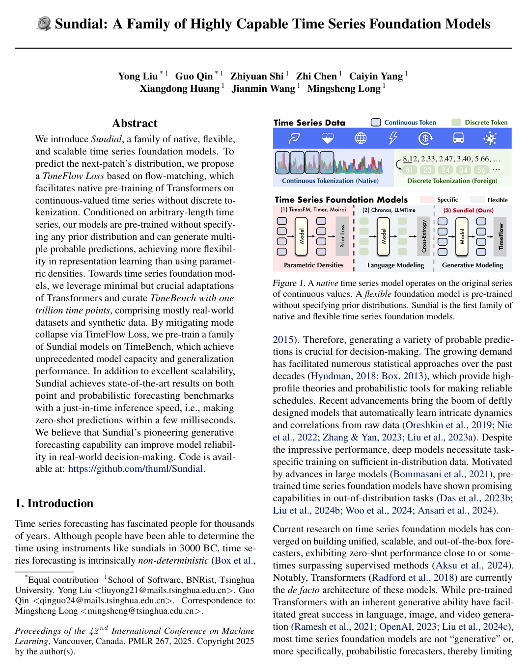
We introduce Sundial, a family of native, flexible, and scalable time series foundation models. To predict the next-patch's distribution, we propose a TimeFlow Loss based on flow-matching, which facilitates native pre-training of Transformers on continuous-valued time series without discrete tokenization. Conditioned on arbitrary-length time series, our models are pre-trained without specifying any prior distribution and can generate multiple probable predictions, achieving more flexibility in representation learning than using parametric densities. Towards time series foundation models, we leverage minimal but crucial adaptations of Transformers and curate TimeBench with one trillion time points, comprising mostly real-world datasets and synthetic data. By mitigating mode collapse via TimeFlow Loss, we pre-train a family of Sundial models on TimeBench, which achieve unprecedented model capacity and generalization performance. In addition to excellent scalability, Sundial achieves state-of-the-art results on both point and probabilistic forecasting benchmarks with a just-in-time inference speed, i.e., making zero-shot predictions within a few milliseconds. We believe that Sundial's pioneering generative forecasting capability can improve model reliability in real-world decision-making. Code is available at: https://github.com/thuml/Sundial.

Topics

encoder-decoder inference probabilistic inference representation learning synthetic data

Keywords

time series foundation models Sundial long-term forecasting datasets probabilistic forecasting autoregressive models deterministic forecasters generative forecasters temporal dynamics forecasting benchmark

1. Introduction
2. Related Work
2.1. Time Series Forecasting
2.2. Time Series Foundation Models
2.3. Generative Modeling for Time Series
3. Preliminaries
3.1. Flow-Matching
3.2. Generative Models for Probabilistic Forecasting
4. Approach
4.1. Sundial
4.1.1. TIME SERIES TOKENIZATION
4.1.2. TRANSFORMER BACKBONE
4.1.3. TIMEFLOW LOSS
4.2. TimeBench
5. Experiments
5.1. Time Series Forecasting
5.1.1. POINT FORECASTING
5.1.2. PROBABILISTIC FORECASTING
5.2. Scalability
5.3. TimeFlow Loss
5.4. Test-Time Calibration
5.5. Model Adaptation
5.6. Ablation Study
6. Conclusion
Acknowledgements
Impact Statement
References
A. Dataset Statistics
B. Implementation Details
C. Supplementary Results
C.1. Discussion of Mode Collapse
C.2. Scaling Behavior Using More Data
C.3. Performance with Varying Lookback Lengths
C.4. Zero-Shot Results of Point Forecasting
C.5. Zero-Shot Results on GIFT-Eval and FEV Leaderboard
D. Showcases
D.1. Showcases of Sundial
D.2. Showcases of Generative Forecasters and Deterministic Forecasters
E. Limitations
F. Societal Impacts
F.1. Real-World Applications
F.2. Academic Research

Knowls

Knowl 1 — Sundial Architecture and Continuous Tokenization
model/method
Sundial is a family of autoregressive, continuous-valued generative foundation models for time series forecasting. Given a univariate time series $X = \{x_1, \dots, x_T\} \in \mathbb{R}^T$ , non-stationarity and outlier range shifts are addressed by applying a two-stage instance normalization (re-normalization) within each sample. The normalized sequence is partitioned into non-overlapping patches $x_i = X_{1+(i-1)P : iP} \in \mathbb{R}^P$ of length $P$ .

To accommodate arbitrary sequence lengths $T$ that are not evenly divisible by $P$ , the series is padded at the start, and a binary mask $m_i \in \{0, 1\}^P$ is concatenated to each patch to indicate valid versus padded positions. This yields $N = \lceil T/P \rceil$ patch tokens. Each token is projected into a continuous $D$ -dimensional representation using a shared Multi-Layer Perceptron (MLP): $h_i^{(0)} = \text{PatchEmbed}(\text{Concat}(x_i, m_i)) \in \mathbb{R}^D$

These embeddings are processed by a decoder-only Transformer backbone employing Pre-Layer Normalization (Pre-LN), FlashAttention, and Rotary Position Embeddings (RoPE). Causal self-attention at each layer is computed as: $A_{ij} = h_i^\top W_q R_{\Theta, i-j} W_k^\top h_j$ $\text{Attention}(H) = \text{Softmax}\left(\frac{\text{Mask}(A)}{\sqrt{d}}\right) H W_v$ where $W_q, W_k, W_v \in \mathbb{R}^{D \times d}$ map token representations $H = \{h_i\}$ to queries, keys, and values of dimension $d$ , $R_{\Theta, t} \in \mathbb{R}^{d \times d}$ is the rotary matrix for relative offset $t = i - j$ , and $\text{Mask}(\cdot)$ enforces autoregressive causal masking.

From the top Transformer layer representation $h_i \in \mathbb{R}^D$ , Sundial outputs a multi-patch prediction horizon $\hat{y}_i = \hat{X}_{1+iP : iP+F} \in \mathbb{R}^F$ where $F > P$ , reducing the number of autoregressive steps required for long-horizon generation.
Knowl 2 — TimeFlow Loss for Continuous Autoregressive Flow-Matching
equation
To learn multi-modal predictive distributions on continuous-valued time series without discrete bucket quantization or fixed parametric distribution priors (such as unimodal or mixture Gaussian densities), Sundial trains using TimeFlow Loss based on conditional flow-matching.

Let $h_i \in \mathbb{R}^D$ be the sequence representation at token position $i$ produced by the Transformer backbone. Let $y_i \in \mathbb{R}^F$ denote the ground-truth future patch trajectory of length $F$ , and let $y_i^{(0)} \sim \mathcal{N}(0, I_F)$ be a standard Gaussian noise vector. A flow timestep $t$ is sampled uniformly from $\mathcal{U}[0, 1]$ , and an intermediate state along the conditional optimal-transport linear probability path is formed as: $y_i^{(t)} = t y_i + (1 - t) y_i^{(0)}$

A velocity network $\text{FM-Net}(y_i^{(t)}, t, h_i)$ parameterized by weights $\theta$ predicts the time-dependent velocity field. The context representation $h_i$ acts as a time-invariant conditioning signal across $t \in [0, 1]$ and is modulated into the layers of $\text{FM-Net}$ via Adaptive Layer Normalization (AdaLN).

The total TimeFlow Loss across all $N$ token positions in a sequence is defined as: $\mathcal{L}_{\text{TimeFlow}} = \sum_{i=1}^N \left\| \text{FM-Net}\left(y_i^{(t)}, t, h_i\right) - \left(y_i - y_i^{(0)}\right) \right\|_2^2$

This regression objective aligns the vector field with the optimal transport path $(y_i - y_i^{(0)})$ , allowing the model to fit arbitrary target densities and avoiding mode collapse during large-scale pre-training.
Knowl 3 — TimeFlow Sampling Procedure for Generative Forecasting
algorithm
During inference, Sundial generates future forecast trajectories by numerically integrating the ordinary differential equation defined by the learned velocity field $\text{FM-Net}$ , initialized from standard Gaussian noise. Generating multiple forecast samples shares the lookback condition representation $h_i$ without repeating the Transformer backbone forward pass.
Input: Lookback condition vector $h_i \in \mathbb{R}^D$ , integration steps $K \in \mathbb{Z}^+$
Output: Predicted sequence patch $\hat{y}_i \in \mathbb{R}^F$
$\hat{y}_i \sim \mathcal{N}(0, I_F)$
$\Delta t \leftarrow 1 / K$
for $k \leftarrow 0$ to $K - 1$ do
$\hat{y}_i \leftarrow \hat{y}_i + \text{FM-Net}(\hat{y}_i, k \cdot \Delta t, h_i) \cdot \Delta t$
end for
return $\hat{y}_i$
To construct probabilistic forecasts (such as the median path and prediction intervals at specified quantiles), $S$ independent initial noise vectors $\hat{y}_i^{(0)} \sim \mathcal{N}(0, I_F)$ are drawn and passed through the integration loop in parallel using the shared context $h_i$ . By default, evaluations utilize $K = 50$ steps and $S \in \{20, 100\}$ trajectory samples.

Knowl 4 — Sundial Model Family Configurations

model/method

The Sundial foundation model family is instantiated in three scale configurations (Small, Base, Large), pairing a decoder-only Transformer backbone with an AdaLN-conditioned flow-matching Multi-Layer Perceptron (FM-Net).

Model	Patch Size $P$	Context $T$	Prediction Horizon $F$	Layers $L$	Hidden $(D, D_{\text{ff}})$	Heads $H$	FM-Net $(D_{\text{tf}}, L_{\text{tf}})$	Parameters
Sundial $_{\text{Small}}$	16	2880	$\{16, 720\}$	6	$(512, 2048)$	8	$(512, 3)$	32M
Sundial $_{\text{Base}}$	16	2880	$\{16, 720\}$	12	$(768, 3072)$	12	$(768, 3)$	128M
Sundial $_{\text{Large}}$	16	2880	$\{16, 720\}$	24	$(1024, 4096)$	16	$(1024, 6)$	444M

Here, $P$ is the input patch length, $T$ is the maximum input context length, $F$ is the multi-patch prediction horizon ( $F = 16$ for short-term benchmarks and $F = 720$ for long-term benchmarks), $L$ is the number of Transformer layers, $D$ is the embedding dimension, $D_{\text{ff}}$ is the feed-forward network hidden dimension, $H$ is the number of multi-head self-attention heads, $D_{\text{tf}}$ is the hidden dimension of FM-Net, and $L_{\text{tf}}$ is the number of layers in FM-Net.

Knowl 5 — Composition of the TimeBench Pre-Training Dataset

data/table

TimeBench is a curated multi-domain pre-training corpus containing over 1.032 trillion ( $1032\text{B}$ ) time points spanning multiple temporal resolutions, real-world sectors, and synthetic patterns.

Data Source	Time Points (# Pts.)	Ratio (%)
Chronos	94B	9.11%
ECG	48B	4.65%
Finance	10.5B	1.02%
IoT	5.8B	0.56%
LOTSA	230B	22.29%
Synthetic (KernelSynth)	0.5B	0.05%
ERA5 3h	129B	12.50%
ERA5 12h	32B	3.10%
ERA5 Daily	406B	39.35%
ERA5 Weekly	58B	5.62%
ERA5 Monthly	13.5B	1.31%
ERA5 Quarterly	4.5B	0.44%
Total	1032B	100.00%

All test splits from downstream evaluation benchmarks (including Time-Series-Library, GIFT-Eval, and FEV) are excluded from TimeBench to enforce strict zero-shot evaluation.

Knowl 6 — Zero-Shot Forecasting Performance on Time-Series-Library (TSLib)

data/table

Sundial models were evaluated zero-shot on six long-term forecasting datasets from Time-Series-Library across four forecasting horizons $\{96, 192, 336, 720\}$ with a context length of 2880. The table below reports the average Mean Squared Error (MSE) and Mean Absolute Error (MAE) across the four prediction lengths for each dataset, along with the total count of 1st-place rankings across all 24 individual evaluation settings (6 datasets $\times$ 4 horizons).

Model	ETTm1		ETTm2		ETTh1		ETTh2		ECL		Weather		1st Count
	MSE	MAE	MSE	MAE	MSE	MAE	MSE	MAE	MSE	MAE	MSE	MAE	MSE	MAE
Sundial $_{\text{Small}}$ (32M)	0.354	0.388	0.265	0.324	0.390	0.418	0.340	0.387	0.169	0.265	0.233	0.271	7	2
Sundial $_{\text{Base}}$ (128M)	0.336	0.377	0.258	0.320	0.411	0.434	0.333	0.387	0.169	0.265	0.234	0.270	8	5
Sundial $_{\text{Large}}$ (444M)	0.331	0.369	0.254	0.315	0.395	0.420	0.334	0.387	0.166	0.262	0.238	0.275	16	16
Time-MoE $_{\text{Base}}$	0.394	0.415	0.317	0.365	0.400	0.424	0.366	0.404	-	-	0.265	0.297	0	1
Time-MoE $_{\text{Large}}$	0.376	0.405	0.316	0.361	0.394	0.419	0.405	0.415	-	-	0.270	0.300	0	0
Time-MoE $_{\text{Ultra}}$	0.356	0.391	0.288	0.344	0.412	0.426	0.371	0.399	-	-	0.256	0.288	2	1
Timer-XL	0.373	0.392	0.273	0.336	0.404	0.417	0.347	0.388	0.174	0.278	0.256	0.294	1	3
Moirai $_{\text{Base}}$	0.406	0.385	0.311	0.337	0.417	0.419	0.362	0.382	0.187	0.274	0.287	0.281	0	2
Moirai $_{\text{Large}}$	0.422	0.391	0.329	0.343	0.480	0.439	0.367	0.377	0.186	0.270	0.264	0.273	0	6
Chronos $_{\text{Base}}$	0.645	0.500	0.310	0.350	0.591	0.468	0.405	0.410	0.214	0.278	0.292	0.315	0	0
Chronos $_{\text{Large}}$	0.555	0.465	0.295	0.338	0.588	0.466	0.455	0.427	0.204	0.273	0.279	0.306	0	0
TimesFM	0.433	0.418	0.328	0.346	0.473	0.443	0.392	0.406	-	-	-	-	0	0

Sundial $_{\text{Large}}$ attains 16 first-place rankings in MSE and 16 in MAE across the 24 settings. Relative to Time-MoE, the Sundial model family achieves an average MSE reduction of 7.57% and MAE reduction of 4.71%.

Knowl 7 — Zero-Shot Probabilistic Performance on GIFT-Eval and FEV
empirical result
Sundial was evaluated on two probabilistic zero-shot forecasting benchmarks:
1. GIFT-Eval: Across 23 diverse datasets spanning 97 forecasting configurations (using 100 generated trajectories), Sundial achieves a Mean Absolute Scaled Error (MASE) of 0.673, ranking 1st among 14 evaluated models. It outperforms supervised models such as PatchTST (MASE 0.762) and iTransformer (MASE 0.802), as well as foundation models including TimesFM (MASE 0.680), TabPFN (MASE 0.748), Chronos (MASE 0.786), and Moirai (MASE 0.809). On Continuous Ranked Probability Score (CRPS), Sundial achieves 0.472, ranking 2nd overall (behind TimesFM at 0.465, while outperforming Chronos at 0.551 and Moirai at 0.515), with an overall benchmark rank of 9.062.
2. FEV Leaderboard: Across 27 unseen probabilistic datasets evaluated with 20 sample paths, Sundial outperforms 70% of task-specific models trained in-distribution. Furthermore, due to continuous patch tokenization and multi-patch prediction ( $F=16$ ), Sundial achieves a $35\times$ inference speedup over Chronos, matching the inference speed of non-autoregressive supervised architectures such as N-BEATS.

Knowl 8 — Comparison of Training Objectives: TimeFlow vs. Diffusion vs. MSE

empirical result

Using identical Transformer backbone architectures and pre-training data scales on TimeBench, models pre-trained using TimeFlow Loss were compared to models trained with Denoising Diffusion Loss and Mean Squared Error (MSE) Loss on TSLib point forecasting (MSE) and GIFT-Eval probabilistic forecasting (CRPS).

Objective	Zero-Shot MSE (TSLib)						Avg. MSE	GIFT-Eval CRPS
	ETTm1	ETTm2	ETTh1	ETTh2	ECL	Weather
TimeFlow	0.336	0.258	0.411	0.333	0.169	0.234	0.290	0.5050
Diffusion	0.362	0.265	0.444	0.360	0.202	0.252	0.314	0.5340
MSE	0.360	0.264	0.404	0.341	0.175	0.231	0.296	0.6420

TimeFlow Loss achieves the lowest average MSE (0.290 versus 0.314 for Diffusion and 0.296 for MSE) and the lowest probabilistic error on GIFT-Eval (CRPS of 0.5050 versus 0.5340 for Diffusion and 0.6420 for MSE). Deterministic MSE loss pre-specifies a unimodal predictive distribution that causes mode collapse on heterogeneous time series, manifesting as over-smoothed predictions. TimeFlow captures complex multi-modal predictive densities while delivering higher sample fidelity and training stability than diffusion denoising.

Knowl 9 — Test-Time Calibration and Architectural Component Ablations in Sundial
empirical result
Sundial exhibits test-time calibration and efficiency properties across several architectural configurations:
1. Sample Count and Integration Step Calibration: On the FEV benchmark, drawing more prediction samples $S$ during inference improves calibration: increasing $S$ from 10 to 100 decreases MASE from $\approx 0.851$ to $0.830$ and Weighted Quantile Loss (WQL) from $\approx 0.718$ to $0.687$ . Increasing flow-matching ODE sampling steps $K$ from 5 to 50 decreases MASE from $\approx 0.842$ to $0.834$ and WQL from $\approx 0.712$ to $0.694$ .
2. Rotary Position Embedding (RoPE): Incorporating RoPE reduces average TSLib zero-shot MSE from $\approx 0.303$ to $0.290$ and MAE from $\approx 0.360$ to $0.342$ .
3. Pre-Layer Normalization (Pre-LN): Pre-LN scales stably with training iterations on TSLib (MSE decreases from $\approx 0.297$ at 15k iterations to $0.290$ at 30k iterations), whereas Post-LN degrades performance as training progresses (MSE increases from $\approx 0.330$ at 15k iterations to $\approx 0.334$ at 30k iterations).
4. FlashAttention and KV Cache: FlashAttention reduces peak GPU memory footprint during pre-training by 14.8%, while KV Cache accelerates autoregressive generation speed during inference by 43.6%, both with zero loss in prediction accuracy.
Knowl 10 — Limitations of the Sundial Model Family
limitation
The authors identify four principal limitations of the Sundial framework:
1. High-Frequency Generalization: Because TimeBench is primarily composed of middle- and low-frequency time series, zero-shot forecasting quality on very high-frequency datasets is not guaranteed, and generated paths can produce hallucinations.
2. Naive Sampling Strategy: Inference is conducted via standard uniform ODE integration starting from random Gaussian noise without frequency-domain normalization or advanced guidance/sampling techniques.
3. Univariate Pre-Training: Sundial processes multivariate data as flattened, independent univariate series (via the S3 format), which ignores explicit cross-variate correlations and external covariate interactions.
4. Autoregressive Error Accumulation: While autoregressive patching enables flexible context lengths, multi-step autoregressive rolling rollouts over long forecasting horizons can lead to error drift and over-smoothed predictions.

Coverage note — Qualitative visual showcase plots from the appendix were omitted as their quantitative conclusions are comprehensively captured in the empirical performance tables, calibration analyses, and limitation knowls.

References

1.Aksu, T., Woo, G., Liu, J., Liu, X., Liu, C., Savarese, S., Xiong, C., and Sahoo, D. Gift-eval: A benchmark for general time series forecasting model evaluation. In NeurIPS Workshop on Time Series in the Age of Large Models, 2024.
2.Ansari, A. F., Stella, L., Turkmen, C., Zhang, X., Mercado, P., Shen, H., Shchur, O., Rangapuram, S. S., Arango, S. P., Kapoor, S., et al. Chronos: Learning the language of time series. arXiv preprint arXiv:2403.07815, 2024.
3.Baevski, A. and Auli, M. Adaptive input representations for neural language modeling. arXiv preprint arXiv:1809.10853, 2018.
4.Bai, S., Kolter, J. Z., and Koltun, V. An empirical evaluation of generic convolutional and recurrent networks for sequence modeling. arXiv preprint arXiv:1803.01271, 2018.
5.Bengio, Y., Ducharme, R., and Vincent, P. A neural probabilistic language model. Advances in neural information processing systems, 13, 2000.
6.Bommasani, R., Hudson, D. A., Adeli, E., Altman, R., Arora, S., von Arx, S., Bernstein, M. S., Bohg, J., Bosselut, A., Brunskill, E., et al. On the opportunities and risks of foundation models. arXiv preprint arXiv:2108.07258, 2021.
7.Box, G. Box and jenkins: time series analysis, forecasting and control. In A Very British Affair: Six Britons and the Development of Time Series Analysis During the 20th Century, pp. 161–215. Springer, 2013.
8.Box, G. E., Jenkins, G. M., Reinsel, G. C., and Ljung, G. M. Time series analysis: forecasting and control. John Wiley & Sons, 2015.
9.Dao, T., Fu, D., Ermon, S., Rudra, A., and Ré, C. Flashattention: Fast and memory-efficient exact attention with io-awareness. Advances in Neural Information Processing Systems, 35:16344–16359, 2022.
10.Das, A., Kong, W., Leach, A., Sen, R., and Yu, R. Long-term forecasting with tide: Time-series dense encoder. arXiv preprint arXiv:2304.08424, 2023a.
11.Das, A., Kong, W., Sen, R., and Zhou, Y. A decoder-only foundation model for time-series forecasting. arXiv preprint arXiv:2310.10688, 2023b.
12.Esser, P., Kulal, S., Blattmann, A., Entezari, R., Müller, J., Saini, H., Levi, Y., Lorenz, D., Sauer, A., Boesel, F., et al. Scaling rectified flow transformers for high-resolution image synthesis. In Forty-first International Conference on Machine Learning, 2024.
13.Goldberger, A. L., Amaral, L. A., Glass, L., Hausdorff, J. M., Ivanov, P. C., Mark, R. G., Mietus, J. E., Moody, G. B., Peng, C.-K., and Stanley, H. E. Physiobank, physiotoolkit, and physionet: components of a new research resource for complex physiologic signals. circulation, 101(23):e215–e220, 2000.
14.Goswami, M., Szafer, K., Choudhry, A., Cai, Y., Li, S., and Dubrawski, A. Moment: A family of open time-series foundation models. arXiv preprint arXiv:2402.03885, 2024.
15.Gruver, N., Finzi, M., Qiu, S., and Wilson, A. G. Large language models are zero-shot time series forecasters. arXiv preprint arXiv:2310.07820, 2023.
16.Gruver, N., Finzi, M., Qiu, S., and Wilson, A. G. Large language models are zero-shot time series forecasters. Advances in Neural Information Processing Systems, 36, 2024.
17.Hersbach, H., Bell, B., Berrisford, P., Hirahara, S., Horányi, A., Muñoz-Sabater, J., Nicolas, J., Peubey, C., Radu, R., Schepers, D., et al. The era5 global reanalysis. Quarterly Journal of the Royal Meteorological Society, 146(730):1999–2049, 2020.
18.Hoo, S. B., Müller, S., Salinas, D., and Hutter, F. The tabular foundation model tabpfn outperforms specialized time series forecasting models based on simple features. arXiv preprint arXiv:2501.02945, 2025.
19.Hyndman, R. Forecasting: principles and practice. OTexts, 2018.
20.Ke, G., Meng, Q., Finley, T., Wang, T., Chen, W., Ma, W., Ye, Q., and Liu, T.-Y. Lightgbm: A highly efficient gradient boosting decision tree. Advances in neural information processing systems, 30, 2017.
21.Kim, T., Kim, J., Tae, Y., Park, C., Choi, J.-H., and Choo, J. Reversible instance normalization for accurate time-series forecasting against distribution shift. In International Conference on Learning Representations, 2021.
22.Kingma, D. P. and Ba, J. Adam: A method for stochastic optimization. arXiv preprint arXiv:1412.6980, 2014.
23.Kollovieh, M., Lienen, M., Lüdke, D., Schwinn, L., and Günnemann, S. Flow matching with gaussian process priors for probabilistic time series forecasting. arXiv preprint arXiv:2410.03024, 2024.
24.Li, T., Tian, Y., Li, H., Deng, M., and He, K. Autoregressive image generation without vector quantization. arXiv preprint arXiv:2406.11838, 2024.
25.Liang, Y., Wen, H., Nie, Y., Jiang, Y., Jin, M., Song, D., Pan, S., and Wen, Q. Foundation models for time series analysis: A tutorial and survey. In Proceedings of the 30th ACM SIGKDD conference on knowledge discovery and data mining, pp. 6555–6565, 2024.
26.Lim, B., Arık, S. O., Loeff, N., and Pfister, T. Temporal fusion transformers for interpretable multi-horizon time series forecasting. International Journal of Forecasting, 37(4):1748–1764, 2021.
27.Lipman, Y., Chen, R. T., Ben-Hamu, H., Nickel, M., and Le, M. Flow matching for generative modeling. arXiv preprint arXiv:2210.02747, 2022.
28.Lipman, Y., Havasi, M., Holderrieth, P., Shaul, N., Le, M., Karrer, B., Chen, R. T., Lopez-Paz, D., Ben-Hamu, H., and Gat, I. Flow matching guide and code. arXiv preprint arXiv:2412.06264, 2024.
29.Liu, Y., Wu, H., Wang, J., and Long, M. Non-stationary transformers: Exploring the stationarity in time series forecasting. Advances in Neural Information Processing Systems, 35:9881–9893, 2022.
30.Liu, Y., Hu, T., Zhang, H., Wu, H., Wang, S., Ma, L., and Long, M. itransformer: Inverted transformers are effective for time series forecasting. arXiv preprint arXiv:2310.06625, 2023a.
31.Liu, Y., Li, C., Wang, J., and Long, M. Koopa: Learning non-stationary time series dynamics with koopman predictors. arXiv preprint arXiv:2305.18803, 2023b.
32.Liu, Y., Qin, G., Huang, X., Wang, J., and Long, M. Timer-xl: Long-context transformers for unified time series forecasting. arXiv preprint arXiv:2410.04803, 2024a.
33.Liu, Y., Zhang, H., Li, C., Huang, X., Wang, J., and Long, M. Timer: Generative pre-trained transformers are large time series models. In Forty-first International Conference on Machine Learning, 2024b.
34.Liu, Y., Zhang, K., Li, Y., Yan, Z., Gao, C., Chen, R., Yuan, Z., Huang, Y., Sun, H., Gao, J., et al. Sora: A review on background, technology, limitations, and opportunities of large vision models. arXiv preprint arXiv:2402.17177, 2024c.
35.Muñoz-Sabater, J., Dutra, E., Agustí-Panareda, A., Albergel, C., Arduini, G., Balsamo, G., Boussetta, S., Choulga, M., Harrigan, S., Hersbach, H., et al. Era5-land: A state-of-the-art global reanalysis dataset for land applications. Earth system science data, 13(9):4349–4383, 2021.
36.Nie, Y., Nguyen, N. H., Sinthong, P., and Kalagnanam, J. A time series is worth 64 words: Long-term forecasting with transformers. arXiv preprint arXiv:2211.14730, 2022.
37.OpenAI, R. Gpt-4 technical report. arxiv 2303.08774. View in Article, 2:13, 2023.
38.Oreshkin, B. N., Carpov, D., Chapados, N., and Bengio, Y. N-beats: Neural basis expansion analysis for interpretable time series forecasting. arXiv preprint arXiv:1905.10437, 2019.
39.Paszke, A., Gross, S., Massa, F., Lerer, A., Bradbury, J., Chanan, G., Killeen, T., Lin, Z., Gimelshein, N., Antiga, L., et al. Pytorch: An imperative style, high-performance deep learning library. Advances in neural information processing systems, 32, 2019.
40.Peebles, W. and Xie, S. Scalable diffusion models with transformers. In Proceedings of the IEEE/CVF International Conference on Computer Vision, pp. 4195–4205, 2023.
41.PEMS. Traffic Dataset. http://pems.dot.ca.gov/.
42.Pope, R., Douglas, S., Chowdhery, A., Devlin, J., Bradbury, J., Heek, J., Xiao, K., Agrawal, S., and Dean, J. Efficiently scaling transformer inference. Proceedings of Machine Learning and Systems, 5:606–624, 2023.
43.Radford, A., Narasimhan, K., Salimans, T., Sutskever, I., et al. Improving language understanding by generative pre-training. OpenAI, 2018.
44.Ramesh, A., Pavlov, M., Goh, G., Gray, S., Voss, C., Radford, A., Chen, M., and Sutskever, I. Zero-shot text-to-image generation. In International conference on machine learning, pp. 8821–8831. Pmlr, 2021.
45.Rasley, J., Rajbhandari, S., Ruwase, O., and He, Y. Deepspeed: System optimizations enable training deep learning models with over 100 billion parameters. In Proceedings of the 26th ACM SIGKDD International Conference on Knowledge Discovery & Data Mining, pp. 3505–3506, 2020.
46.Rasul, K., Seward, C., Schuster, I., and Vollgraf, R. Autoregressive denoising diffusion models for multivariate probabilistic time series forecasting. In International Conference on Machine Learning, pp. 8857–8868. PMLR, 2021.
47.Rasul, K., Ashok, A., Williams, A. R., Khorasani, A., Adamopoulos, G., Bhagwatkar, R., Biloš, M., Ghonia, H., Hassen, N. V., Schneider, A., et al. Lag-llama: Towards foundation models for time series forecasting. arXiv preprint arXiv:2310.08278, 2023.
48.Rombach, R., Blattmann, A., Lorenz, D., Esser, P., and Ommer, B. High-resolution image synthesis with latent diffusion models. In Proceedings of the IEEE/CVF conference on computer vision and pattern recognition, pp. 10684–10695, 2022.
49.Salinas, D., Flunkert, V., Gasthaus, J., and Januschowski, T. Deepar: Probabilistic forecasting with autoregressive recurrent networks. International journal of forecasting, 36(3):1181–1191, 2020.
50.Shen, L. and Kwok, J. Non-autoregressive conditional diffusion models for time series prediction. In International Conference on Machine Learning, pp. 31016–31029. PMLR, 2023.
51.Shi, J., Ma, Q., Ma, H., and Li, L. Scaling law for time series forecasting. arXiv preprint arXiv:2405.15124, 2024a.
52.Shi, X., Wang, S., Nie, Y., Li, D., Ye, Z., Wen, Q., and Jin, M. Time-moe: Billion-scale time series foundation models with mixture of experts. arXiv preprint arXiv:2409.16040, 2024b.
53.Shoeybi, M., Patwary, M., Puri, R., LeGresley, P., Casper, J., and Catanzaro, B. Megatron-lm: Training multibillion parameter language models using model parallelism. arXiv preprint arXiv:1909.08053, 2019.
54.Sohl-Dickstein, J., Weiss, E., Maheswaranathan, N., and Ganguli, S. Deep unsupervised learning using nonequilibrium thermodynamics. In International conference on machine learning, pp. 2256–2265. PMLR, 2015.
55.Su, J., Ahmed, M., Lu, Y., Pan, S., Bo, W., and Liu, Y. Roformer: Enhanced transformer with rotary position embedding. Neurocomputing, 568:127063, 2024.
56.Tashiro, Y., Song, J., Song, Y., and Ermon, S. Csdi: Conditional score-based diffusion models for probabilistic time series imputation. Advances in Neural Information Processing Systems, 34:24804–24816, 2021.
57.Tong, A., Fatras, K., Malkin, N., Huguet, G., Zhang, Y., Rector-Brooks, J., Wolf, G., and Bengio, Y. Improving and generalizing flow-based generative models with minibatch optimal transport. arXiv preprint arXiv:2302.00482, 2023.
58.Touvron, H., Lavril, T., Izacard, G., Martinet, X., Lachaux, M.-A., Lacroix, T., Rozière, B., Goyal, N., Hambro, E., Azhar, F., et al. Llama: Open and efficient foundation language models. arXiv preprint arXiv:2302.13971, 2023.
59.Vovk, V., Gammerman, A., and Shafer, G. Algorithmic learning in a random world, volume 29. Springer, 2005.
60.Wei, J., Bosma, M., Zhao, V. Y., Guu, K., Yu, A. W., Lester, B., Du, N., Dai, A. M., and Le, Q. V. Finetuned language models are zero-shot learners. arXiv preprint arXiv:2109.01652, 2021.
61.Wen, R., Torkkola, K., Narayanaswamy, B., and Madeka, D. A multi-horizon quantile recurrent forecaster. arXiv preprint arXiv:1711.11053, 2017.
62.Woo, G., Liu, C., Kumar, A., Xiong, C., Savarese, S., and Sahoo, D. Unified training of universal time series forecasting transformers. arXiv preprint arXiv:2402.02592, 2024.
63.Wu, H., Xu, J., Wang, J., and Long, M. Autoformer: Decomposition transformers with auto-correlation for long-term series forecasting. Advances in Neural Information Processing Systems, 34:22419–22430, 2021.
64.Wu, H., Hu, T., Liu, Y., Zhou, H., Wang, J., and Long, M. Timesnet: Temporal 2d-variation modeling for general time series analysis. arXiv preprint arXiv:2210.02186, 2022.
65.Xiong, R., Yang, Y., He, D., Zheng, K., Zheng, S., Xing, C., Zhang, H., Lan, Y., Wang, L., and Liu, T. On layer normalization in the transformer architecture. In International Conference on Machine Learning, pp. 10524–10533. PMLR, 2020.
66.Zhang, R., Isola, P., Efros, A. A., Shechtman, E., and Wang, O. The unreasonable effectiveness of deep features as a perceptual metric. In Proceedings of the IEEE conference on computer vision and pattern recognition, pp. 586–595, 2018.
67.Zhang, Y. and Yan, J. Crossformer: Transformer utilizing cross-dimension dependency for multivariate time series forecasting. In The eleventh international conference on learning representations, 2023.
68.Zhao, W. X., Zhou, K., Li, J., Tang, T., Wang, X., Hou, Y., Min, Y., Zhang, B., Zhang, J., Dong, Z., et al. A survey of large language models. arXiv preprint arXiv:2303.18223, 2023.

Citation

MLA

Liu, Y., et al. “Sundial: A Family of Highly Capable Time Series Foundation Models”. arXiv, 2025, https://doi.org/10.48550/arxiv.2502.00816.

APA

Liu, Y., Qin, G., Shi, Z., Chen, Z., Yang, C., Huang, X., Wang, J., & Long, M. (2025). Sundial: A Family of Highly Capable Time Series Foundation Models. arXiv. https://doi.org/10.48550/arxiv.2502.00816

Chicago

Liu, Y., G. Qin, Z. Shi, et al. 2025. “Sundial: A Family of Highly Capable Time Series Foundation Models”. Preprint, ArXiv. https://doi.org/10.48550/arxiv.2502.00816.

Harvard

Liu, Y. et al. (2025) “Sundial: A Family of Highly Capable Time Series Foundation Models”. arXiv. Available at: https://doi.org/10.48550/arxiv.2502.00816.

Vancouver

1. Liu Y, Qin G, Shi Z, Chen Z, Yang C, Huang X, Wang J, Long M (2025) Sundial: A Family of Highly Capable Time Series Foundation Models. https://doi.org/10.48550/arxiv.2502.00816

BibTeX

@misc{https://doi.org/10.48550/arxiv.2502.00816,
  doi = {10.48550/ARXIV.2502.00816},
  url = {https://arxiv.org/abs/2502.00816},
  author = {Liu, Yong and Qin, Guo and Shi, Zhiyuan and Chen, Zhi and Yang, Caiyin and Huang, Xiangdong and Wang, Jianmin and Long, Mingsheng},
  keywords = {Machine Learning (cs.LG), FOS: Computer and information sciences, FOS: Computer and information sciences},
  title = {Sundial: A Family of Highly Capable Time Series Foundation Models},
  publisher = {arXiv},
  year = {2025},
  copyright = {Creative Commons Attribution Non Commercial No Derivatives 4.0 International}
}

Metadata:DOI registry

Source Code

This paper has an official code repository available. Click below to access the source code.

View Repository

Access the Paper

This paper is available from its original source. Click below to access the PDF.

Open PDF

License: https://creativecommons.org/licenses/by/4.0/

Sundial: A Family of Highly Capable Time Series Foundation Models

Abstract

Topics

Keywords

Table of Contents

Knowls

Knowl 1 — Sundial Architecture and Continuous Tokenization

Knowl 2 — TimeFlow Loss for Continuous Autoregressive Flow-Matching

Knowl 3 — TimeFlow Sampling Procedure for Generative Forecasting