Prototypical Residual Networks for Anomaly Detection and Localization

Hui ZhangZuxuan WuZheng WangZhineng ChenYu-Gang Jiang

article2023CVPR109 citations

Proposes a prototypical residual network that captures multi-scale feature deviations and variable-sized defects to achieve state-of-the-art anomaly detection and precise pixel-level localization across industrial benchmarks.

Listen

Automated visual inspection is critical for quality control in modern manufacturing, medical imaging, and surveillance. However, industrial computer vision systems face significant challenges because defective samples are exceptionally rare, subtle, and highly variable in shape and size. Existing unsupervised methods, which learn only from normal samples, frequently yield coarse predictions and false alarms, while existing supervised approaches struggle with extreme data imbalance and fail to pinpoint exact defect boundaries.

To resolve these problems, the article introduces the Prototypical Residual Network (PRN), a supervised deep learning framework designed to simultaneously achieve high-precision anomaly detection (identifying whether an image contains a defect) and anomaly localization (pinpointing exact defective pixels). PRN learns explicit feature differences—or residuals—between anomalous images and representative normal visual patterns across multiple spatial resolutions. The architecture incorporates multi-scale prototypes to model normal textures, a multi-size self-attention mechanism to detect inconsistencies across varying patch sizes, and multi-scale fusion blocks to integrate contextual information. To overcome severe data scarcity, the authors also implement synthetic data generation strategies that augment seen defects and simulate new, unseen anomalies.

The authors evaluated PRN across four benchmark industrial inspection datasets (MVTec AD, DAGM, BTAD, and KolektorSDD2) under a few-shot setting using only 10 abnormal training samples per category. The experimental results demonstrate strong performance advantages. On the primary MVTec AD benchmark, PRN achieved an overall image-level detection accuracy (AUROC) of 99.4% and a pixel-level localization AUROC of 99.0%, surpassing competing supervised and unsupervised models. On the more rigorous Average Precision metric for defect localization, PRN reached 78.6%, outperforming the prior unsupervised benchmark by 10.5 percentage points and the leading supervised method by 52.6 percentage points. Furthermore, PRN processed images in approximately 0.064 seconds per frame, operating 30% to 70% faster than comparable high-performing models.

These findings indicate that learning residual representations against clustered normal prototypes, combined with targeted synthetic anomaly generation, effectively solves the few-shot imbalance bottleneck in visual defect detection. In practical terms, this allows automated inspection systems to achieve superior defect detection reliability and pinpoint accuracy without requiring massive defect-labeling efforts. By significantly reducing false alarms and processing images at higher speeds, the approach can lower production scrap costs, improve throughput, and minimize deployment overhead in automated quality assurance pipelines.

Organizations evaluating automated optical inspection systems should consider adopting residual-based prototype architectures to improve defect localization. Decision-makers planning implementations should first establish pilot deployments on representative assembly lines to validate operational gains against baseline systems. As a key technical consideration, PRN relies on access to accurate ground truth segmentation masks during initial training, and its image-level scoring rule may under-weigh extremely minute flaws. Future engineering efforts should therefore explore automated mask generation and refined scoring mechanisms tailored specifically for micro-defects.

arXiv: 2212.02031
Cover for Prototypical Residual Networks for Anomaly Detection and Localization

Abstract

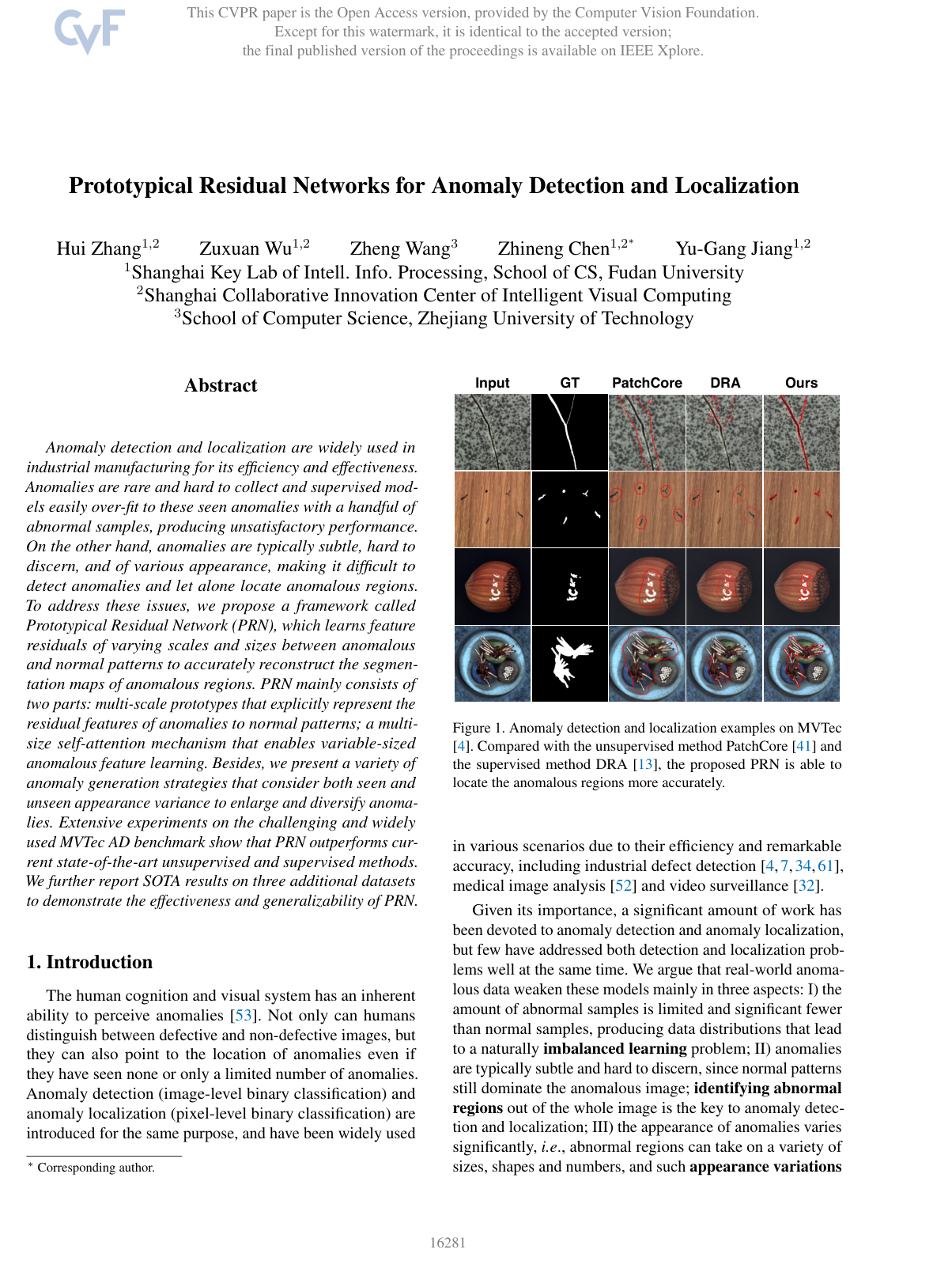
Anomaly detection and localization are widely used in industrial manufacturing for its efficiency and effectiveness. Anomalies are rare and hard to collect and supervised models easily over-fit to these seen anomalies with a handful of abnormal samples, producing unsatisfactory performance. On the other hand, anomalies are typically subtle, hard to discern, and of various appearance, making it difficult to detect anomalies and let alone locate anomalous regions. To address these issues, we propose a framework called Prototypical Residual Network (PRN), which learns feature residuals of varying scales and sizes between anomalous and normal patterns to accurately reconstruct the segmentation maps of anomalous regions. PRN mainly consists of two parts: multi-scale prototypes that explicitly represent the residual features of anomalies to normal patterns; a multi-size self-attention mechanism that enables variable-sized anomalous feature learning. Besides, we present a variety of anomaly generation strategies that consider both seen and unseen appearance variance to enlarge and diversify anomalies. Extensive experiments on the challenging and widely used MVTec AD benchmark show that PRN outperforms current state-of-the-art unsupervised and supervised methods. We further report SOTA results on three additional datasets to demonstrate the effectiveness and generalizability of PRN.

Table of Contents

  • 1. Introduction
  • 2. Related Work
  • 3. Method
  • 3.1. Multi-scale Prototypes
  • 3.2. Multi-scale Fusion
  • 3.3. Multi-size Self-Attention
  • 3.4. Anomaly Generation Strategies
  • 3.5. Training and Inference
  • 4. Experiments
  • 4.1. Experimental Details
  • 4.2. Anomaly Detection and Localization on MVTec
  • 4.3. Ablation Study
  • 4.4. Evaluation on other benchmarks
  • 5. Conclusion
  • References

Knowls

  1. Knowl 1 — Prototypical Residual Network Architecture

    model/method

    Prototypical Residual Network (PRN) is an encoder-decoder network based on a U-Net architecture designed for anomaly detection and pixel-level anomaly localization under few-shot supervised settings.

    The feature encoder is a ResNet-18 pre-trained on ImageNet. Its parameters are frozen during training. The network extracts feature maps from intermediate blocks layer1\text{layer1}, layer2\text{layer2}, and layer3\text{layer3} (denoted as scales j∈{1,2,3}j \in \{1, 2, 3\}) with dimensions 64×64×6464 \times 64 \times 64, 128×32×32128 \times 32 \times 32, and 256×16×16256 \times 16 \times 16 for a 256×256256 \times 256 input image.

    The skip connections between encoder and decoder are modified to perform anomaly residual extraction and multi-scale feature modeling. Specifically, each skip connection incorporates:

    1. Multi-scale Prototypes (MP) to compute residual representations between the input feature maps and pre-computed normal cluster prototypes.
    2. Multi-scale Fusion (MF) blocks to exchange and aggregate features and residuals across different resolution scales.
    3. Multi-size Self-Attention (MSA) blocks to capture patch-level inconsistencies across varying receptive field sizes.

    The decoder consists of upsampling layers and convolutional blocks that process the fused skip-connection features alongside the encoder bottleneck to output a single-channel anomaly segmentation score map Mo∈[0,1]H×W\mathcal{M}_o \in [0, 1]^{H \times W} having the same spatial resolution as the ground-truth anomaly mask M\mathcal{M}.

  2. Knowl 2 — Multi-Scale Prototypes and Residual Representation

    equation

    To capture deviations from normal patterns without losing spatial information, normal representations are constructed as prototype feature maps at multiple scales.

    Let XN\mathcal{X}_N be the set of normal training images (where label yx=0y_x = 0 for all x∈XNx \in \mathcal{X}_N). For each scale j∈{1,2,3}j \in \{1, 2, 3\}, feature maps Fi,j=Fj(xi)∈Rcj×hj×wj\mathcal{F}_{i,j} = \mathcal{F}_j(x_i) \in \mathbb{R}^{c_j \times h_j \times w_j} are extracted using a frozen pre-trained encoder. A set of KK prototypes Pj={Pj1,…,PjK}⊂Rcj×hj×wj\mathcal{P}_j = \{\mathcal{P}_j^1, \dots, \mathcal{P}_j^K\} \subset \mathbb{R}^{c_j \times h_j \times w_j} is initialized by randomly sampling KK feature maps from Fj(XN)\mathcal{F}_j(\mathcal{X}_N) and updating them via kk-means clustering using L2L_2 distance. The number of prototypes KK is set to a fixed proportion (typically 10%10\%) of the total number of normal training samples. Prototypes are frozen during subsequent network training.

    For an input image xix_i, the closest prototype Pj∗\mathcal{P}_j^* at scale jj and its anomalous residual feature representation Di,j∈Rcj×hj×wj\mathcal{D}_{i,j} \in \mathbb{R}^{c_j \times h_j \times w_j} are defined as:

    Di,j=D(Fi,j−Pj∗)\mathcal{D}_{i,j} = D(\mathcal{F}_{i,j} - \mathcal{P}_j^*)

    s.t. Pj∗=arg⁡min⁡Pjk∈Pj∥Fi,j−Pjk∥2\text{s.t. } \mathcal{P}_j^* = \arg\min_{\mathcal{P}_j^k \in \mathcal{P}_j} \|\mathcal{F}_{i,j} - \mathcal{P}_j^k\|_2

    where D(⋅)D(\cdot) computes the element-wise Euclidean distance across channels between the two tensors. Prototypes at each scale jj are matched independently.

  3. Knowl 3 — Multi-Scale Feature and Residual Fusion

    equation

    To exchange spatial and semantic information across intermediate representation scales j∈{1,2,3}j \in \{1, 2, 3\}, Multi-scale Fusion (MF) transforms and sums the feature maps from all three scales.

    The fused feature map Fi,j∗∈Rcj×hj×wj\mathcal{F}_{i,j}^* \in \mathbb{R}^{c_j \times h_j \times w_j} at scale jj is computed as:

    Fi,j∗=f1j(Fi,1)+f2j(Fi,2)+f3j(Fi,3)\mathcal{F}_{i,j}^* = f_{1j}(\mathcal{F}_{i,1}) + f_{2j}(\mathcal{F}_{i,2}) + f_{3j}(\mathcal{F}_{i,3})

    where the transformation function frj(⋅)f_{rj}(\cdot) depends on the source scale index rr and target scale index jj:

    • If r=jr = j: frj(Fi,r)=Fi,rf_{rj}(\mathcal{F}_{i,r}) = \mathcal{F}_{i,r} (identity mapping).
    • If r<jr < j: frj(Fi,r)f_{rj}(\mathcal{F}_{i,r}) downsamples the input feature map via depth-wise separable convolutions with a stride of 2j−r2^{j-r}, kernel size of 2j−r+12^{j-r} + 1, and padding of 2j−r−12^{j-r-1}.
    • If r>jr > j: frj(Fi,r)f_{rj}(\mathcal{F}_{i,r}) upsamples the input feature map via bilinear interpolation followed by a 1×11 \times 1 convolution.

    The residual tensors Di,j\mathcal{D}_{i,j} are fused across scales using the identical MF formulation to produce Di,j∗\mathcal{D}_{i,j}^*. The fused feature map Fi,j∗\mathcal{F}_{i,j}^* and fused residual map Di,j∗\mathcal{D}_{i,j}^* are concatenated along the channel dimension to form Ci,j∗∈R2cj×hj×wj\mathcal{C}_{i,j}^* \in \mathbb{R}^{2c_j \times h_j \times w_j}.

  4. Knowl 4 — Multi-Size Self-Attention Mechanism

    model/method

    To detect localized anomalous inconsistencies across various scales and receptive fields, Multi-size Self-Attention (MSA) operates on the channel-concatenated feature-residual tensor Ci,j∗∈R2cj×hj×wj\mathcal{C}_{i,j}^* \in \mathbb{R}^{2c_j \times h_j \times w_j}.

    MSA splits Ci,j∗\mathcal{C}_{i,j}^* into non-overlapping spatial patches of multiple sizes ps∈{hj,hj/2,hj/4,hj/8}p_s \in \{h_j, h_j/2, h_j/4, h_j/8\}, where each patch size is assigned to a distinct attention head ss. For head ss, patches of shape 2cj×ps×ps2c_j \times p_s \times p_s are extracted and flattened into 1-dimensional vectors of dimension cs=2cj⋅ps2c^s = 2c_j \cdot p_s^2. The total number of patches is N=(hj/ps)×(wj/ps)N = (h_j / p_s) \times (w_j / p_s).

    Linear projection layers map the flattened patch vectors to query embeddings Qi,js∈RN×cs\mathcal{Q}_{i,j}^s \in \mathbb{R}^{N \times c^s}, key embeddings Ki,js∈RN×cs\mathcal{K}_{i,j}^s \in \mathbb{R}^{N \times c^s}, and value embeddings Vi,js∈RN×cs\mathcal{V}_{i,j}^s \in \mathbb{R}^{N \times c^s}. The head attention output Ai,js\mathcal{A}_{i,j}^s is computed via scaled dot-product attention:

    Ai,js=softmax(Qi,js(Ki,js)Tcs)Vi,js\mathcal{A}_{i,j}^s = \text{softmax}\left(\frac{\mathcal{Q}_{i,j}^s (\mathcal{K}_{i,j}^s)^T}{c^s}\right) \mathcal{V}_{i,j}^s

    Each attention tensor Ai,js\mathcal{A}_{i,j}^s is reshaped to the original spatial resolution hj×wjh_j \times w_j. The outputs across all heads are concatenated along the channel dimension and passed through a 2D residual convolutional block to produce Ti,j∈R2cj×hj×wj\mathcal{T}_{i,j} \in \mathbb{R}^{2c_j \times h_j \times w_j}.

    The MSA operation is stacked N=3N = 3 times sequentially, and the final outputs across all scales j∈{1,2,3}j \in \{1, 2, 3\} are fused using another Multi-scale Fusion (MF) block to yield Ti,j∗\mathcal{T}_{i,j}^*, which forms the output of the skip-connection.

  5. Knowl 5 — Online Anomaly Generation Strategies

    algorithm

    To address severe class imbalance in few-shot supervised anomaly detection, PRN uses two complementary online anomaly generation strategies: Extended Anomalies (in-distribution augmentation) and Simulated Anomalies (out-of-distribution augmentation).

    Input: Set of normal samples XNX_N, set of seen anomalous samples XAX_A, texture dataset DTD
    Output: Augmented synthetic training sample EE, ground truth binary mask MM
    function GenerateExtendedAnomaly(XNX_N, XAX_A):
        Sample normal image N∼XNN \sim X_N
        Sample anomalous image Araw∼XAA_{raw} \sim X_A
        Apply color augmentations Aug1Aug_1 to ArawA_{raw} (select two random operations from {equalize, solarize, posterize, sharpness, autocontrast, invert, gamma-contrast}) to obtain AA
        Apply spatial transformation Aug2Aug_2 to AA (random rotate, shear, shift) to obtain RR
        Sample a Target Area (TA) constraint (foreground region for objects; whole image for textures) using geometric shapes {circle, rectangular, polygon}
        Crop RR to TA to produce clipped anomaly region CC
        while RR does not overlap with TA do
            Re-apply Aug2Aug_2 to obtain a new RR
            Crop RR to TA to obtain CC
        end while
        Generate binary mask MM from the non-zero region of CC
        Compute inverted mask Mˉ=1−M\bar{M} = 1 - M
        Sample opacity parameter β∈[0,1]\beta \in [0, 1]
        Synthesize extended anomaly image: E=Mˉ⊙N+(1−β)C+β(M⊙N)E = \bar{M} \odot N + (1 - \beta) C + \beta (M \odot N)
        return E,ME, M
    function GenerateSimulatedAnomaly(XNX_N, DTD):
        Sample normal image N∼XNN \sim X_N
        Generate 2D Perlin noise map PP
        Sample Target Area (TA) with geometric bounds
        Choose anomaly source:
            Case Heterologous (HEA): Sample texture image T∼DTDT \sim \text{DTD}
            Case Homologous (HOA): Sample augmented normal image T∼Aug(XN)T \sim \text{Aug}(X_N)
        Combine noise and texture: C=P⊙TC = P \odot T constrained within TA
        Generate binary mask MM where CC is active
        Blend with normal image NN using opacity β\beta
        return synthetic image and mask MM
  6. Knowl 6 — PRN Training Objective and Anomaly Scoring

    equation

    PRN is trained with pixel-level supervision to minimize the discrepancy between the predicted continuous anomaly score map Mo∈[0,1]H×W\mathcal{M}_o \in [0, 1]^{H \times W} and the binary ground-truth defect mask M∈{0,1}H×W\mathcal{M} \in \{0, 1\}^{H \times W}.

    The overall training loss Ltotal\mathcal{L}_{total} combines Smooth L1L_1 loss and Focal loss:

    Ltotal=SmoothL1(Mo,M)+λLfocal(Mo,M)\mathcal{L}_{total} = \text{Smooth}_{L1}(\mathcal{M}_o, \mathcal{M}) + \lambda \mathcal{L}_{focal}(\mathcal{M}_o, \mathcal{M})

    where λ=5\lambda = 5 is a weighting hyperparameter, Smooth L1L_1 loss reduces sensitivity to outliers, and Focal loss (configured with α=0.5\alpha = 0.5 and focusing parameter γ=4\gamma = 4) mitigates foreground-background pixel imbalance.

    During inference, Mo\mathcal{M}_o directly provides pixel-level anomaly localization scores. For image-level anomaly detection, the image anomaly score S(x)S(x) is computed as the mean of the top-KpixK_{pix} anomalous pixel values in Mo\mathcal{M}_o:

    S(x)=1Kpix∑p∈top-Kpix(Mo)Mo(p)S(x) = \frac{1}{K_{pix}} \sum_{p \in \text{top-}K_{pix}(\mathcal{M}_o)} \mathcal{M}_o(p)

    where Kpix=100K_{pix} = 100 highest-scoring pixels.

  7. Knowl 7 — Anomaly Detection and Localization on MVTec AD Benchmark

    data/table

    Performance of PRN compared to unsupervised and supervised baselines on the MVTec AD benchmark containing 15 sub-datasets (10 object, 5 texture classes). In the supervised setting, each category is provided with only 10 seen abnormal training samples.

    Method Image AUROC (%) Pixel AUROC (%) Pixel PRO (%) Pixel AP (%)
    Unsupervised
    KDAD 88.2 90.0 82.9 25.3
    CFLOW 97.5 97.7 93.4 59.6
    DRAEM 97.6 96.7 91.3 68.1
    SSPCAB 97.1 96.3 90.8 65.5
    CFA 99.1 98.0 92.1 60.0
    RD4AD 98.7 97.8 93.9 55.4
    PatchCore 99.2 98.1 93.9 56.3
    Supervised (10 seen anomalies)
    DevNet 92.2 85.3 71.4 24.4
    DRA 96.1 85.3 73.3 26.0
    PRN (Ours) 99.4 99.0 96.1 78.6

    PRN outperforms previous unsupervised and supervised methods across all four evaluation metrics. On the challenging Pixel Average Precision (AP) metric, PRN surpasses the best unsupervised method (DRAEM) by +10.5%+10.5\% and the best supervised baseline (DRA) by +52.6%+52.6\%. On Per-Region Overlap (PRO), PRN improves over PatchCore and RD4AD by +2.2%+2.2\%.

  8. Knowl 8 — Inference Speed and Performance Comparison on MVTec AD

    data/table

    Comparison of pre-trained feature extractor approaches on MVTec AD evaluated on a single NVIDIA GeForce RTX 3090 GPU, measuring Image AUROC (I), Pixel AUROC (P), Pixel PRO (O), Pixel AP (A), and inference runtime per image in seconds (T).

    Method Backbone I (%) P (%) O (%) A (%) T (s) ↓\downarrow
    CFLOW WideResNet50 97.5 97.7 93.4 59.6 0.127
    RD4AD WideResNet50 98.7 97.8 93.9 55.4 0.094
    PatchCore WideResNet50 99.2 98.1 93.9 56.3 0.133
    CFLOW ResNet-18 96.2 98.1 92.8 59.2 0.106
    RD4AD ResNet-18 97.9 97.1 92.7 53.7 0.076
    DRA ResNet-18 96.1 84.1 71.5 25.7 0.223
    PRN (Ours) ResNet-18 99.4 99.0 96.1 78.6 0.064

    Using a lightweight ResNet-18 backbone, PRN achieves superior detection and localization accuracy while reducing inference latency to 0.064 s0.064\text{ s} per image (1.47×1.47\times faster than RD4AD-ResNet18 and 3.48×3.48\times faster than DRA).

  9. Knowl 9 — Generalization Across Industrial Datasets: DAGM, BTAD, and KolektorSDD2

    data/table

    Evaluation of PRN and competing methods across three additional benchmark datasets (DAGM, BTAD, and KolektorSDD2) with 10 seen abnormal training samples per sub-dataset.

    DAGM BTAD KolektorSDD2
    Method I P O A I P O A I P O A
    DRAEM 91.1 83.4 70.5 35.6 89.0 87.1 61.6 19.2 81.1 85.6 67.9 39.1
    CFLOW 91.2 95.1 87.6 45.2 90.5 96.1 71.6 54.0 95.2 97.4 93.8 46.0
    SSPCAB 90.4 84.5 71.9 33.9 88.3 83.5 54.1 13.0 83.4 86.2 66.1 44.5
    RD4AD 90.7 94.1 85.5 40.8 94.4 96.9 75.8 53.5 96.0 97.6 94.7 43.5
    PatchCore 92.5 96.1 88.0 49.0 92.6 96.9 76.3 51.5 94.6 97.1 89.3 49.8
    DRA 93.5 95.1 88.8 47.6 94.2 75.4 56.2 12.4 86.8 84.4 56.9 3.6
    PRN (Ours) 98.2 96.6 93.8 49.4 94.7 97.1 78.0 54.0 96.4 97.6 94.9 72.5

    Metrics correspond to Image AUROC (I), Pixel AUROC (P), Pixel PRO (O), and Pixel AP (A) in percentage. PRN achieves the best overall performance across all three benchmarks, notably achieving 72.5%72.5\% AP on KolektorSDD2 compared to 49.8%49.8\% for PatchCore and 3.6%3.6\% for DRA.

  10. Knowl 10 — Ablation Analysis of Architectural Modules and Hyperparameters

    empirical result

    Ablation experiments on MVTec AD assess the contribution of architectural components, anomaly generation strategies, prototype proportion, and the number of seen anomaly samples:

    1. Architectural Components (U-Net baseline vs. Modules):

      • U-Net baseline alone achieves: Image AUROC 97.4%97.4\%, Pixel AUROC 91.7%91.7\%, PRO 88.6%88.6\%, AP 58.5%58.5\%.
      • Adding Multi-scale Prototypes (MP), Multi-size Self-Attention (MSA), and Multi-scale Fusion (MF) progressively improves all metrics, with the full PRN reaching Image AUROC 99.4%99.4\%, Pixel AUROC 99.0%99.0\%, PRO 96.1%96.1\%, AP 78.6%78.6\%.
      • Removing MF causes performance to drop to 98.9%98.9\% / 98.5%98.5\% / 95.3%95.3\% / 77.0%77.0\%.
      • Removing MSA drops performance to 97.8%97.8\% / 97.0%97.0\% / 92.1%92.1\% / 74.0%74.0\%.
      • Removing MP drops performance to 98.7%98.7\% / 98.5%98.5\% / 95.4%95.4\% / 78.1%78.1\%.
    2. Anomaly Generation Components:

      • Extended Anomalies (EA) + Target Areas (TA) yields 98.6%98.6\% Image AUROC and 75.7%75.7\% AP.
      • Incorporating Simulated Anomalies via both Heterologous (HEA) and Homologous (HOA) strategies alongside EA and TA maximizes performance (99.4%99.4\% Image AUROC, 78.6%78.6\% AP).
      • Omitting TA constraints degrades AP from 78.6%78.6\% to 77.6%77.6\%.
    3. Prototype Ratio (K/∣XN∣K / |X_N|):

      • Testing prototype proportions of 5%5\%, 10%10\%, 20%20\%, and 100%100\% (where 100%100\% skips clustering and uses all normal samples) shows 10%10\% achieves optimal performance (99.4%99.4\% Image AUROC, 78.6%78.6\% AP, 0.064 s0.064\text{ s} runtime). Setting the ratio to 100%100\% degrades AP sharply to 49.9%49.9\%, demonstrating that cluster centroids provide more robust and noise-free normal descriptors than individual raw sample feature maps.
    4. Number of Seen Training Anomalies:

      • With 1 seen anomaly: PRN achieves Image AUROC 98.8%98.8\%, AP 74.7%74.7\% (vs. DevNet 79.6%/16.5%79.6\% / 16.5\% and DRA 88.9%/19.1%88.9\% / 19.1\%).
      • With 5 seen anomalies: PRN achieves Image AUROC 99.2%99.2\%, AP 76.4%76.4\% (vs. DevNet 86.7%/22.7%86.7\% / 22.7\% and DRA 93.5%/21.9%93.5\% / 21.9\%).
      • With 10 seen anomalies: PRN achieves Image AUROC 99.4%99.4\%, AP 78.6%78.6\% (vs. DevNet 92.2%/24.4%92.2\% / 24.4\% and DRA 96.1%/26.0%96.1\% / 26.0\%).
  11. Knowl 11 — Limitations of Prototypical Residual Networks

    limitation

    Prototypical Residual Networks have two main limitations identified by the authors:

    1. Dependence on Ground-Truth Anomaly Masks: The framework requires accurate pixel-level binary annotation masks for the limited set of seen abnormal training images. In industrial environments where only image-level labels (normal vs. abnormal) are provided without polygon/pixel segmentations, the supervised training objective and extended anomaly generation cannot be directly applied without additional annotation overhead.

    2. Static Top-K Image-Level Scoring: Aggregating image-level anomaly scores via a fixed top-KK pixel average (K=100K=100) assumes a uniform scale of defective area across images. This uniform averaging strategy does not dynamically adapt to anomalous regions that occupy only a tiny fraction of pixels, potentially underestimating the severity of very small or subtle defect instances.

Coverage note — None was omitted. All principal methodological components, mathematical formulations, algorithms, benchmark evaluations, ablation studies, and stated limitations are fully represented.

References

  1. 1.Samet Akcay, Dick Ameln, Ashwin Vaidya, Barath Lakshmanan, Nilesh Ahuja, and Utku Genc. Anomalib: A deep learning library for anomaly detection. arXiv preprint arXiv:2202.08341, 2022. 6
  2. 2.Samet Akcay, Amir Atapour-Abarghouei, and Toby P Breckon. Ganomaly: Semi-supervised anomaly detection via adversarial training. In ACCV, 2018. 3
  3. 3.Samet Akc¸ay, Amir Atapour-Abarghouei, and Toby P Breckon. Skip-ganomaly: Skip connected and adversarially trained encoder-decoder anomaly detection. In IJCNN, 2019. 2
  4. 4.Paul Bergmann, Michael Fauser, David Sattlegger, and Carsten Steger. Mvtec ad–a comprehensive real-world dataset for unsupervised anomaly detection. In CVPR, 2019. 1, 5, 6, 7, 8
  5. 5.Paul Bergmann, Michael Fauser, David Sattlegger, and Carsten Steger. Uninformed students: Student-teacher anomaly detection with discriminative latent embeddings. In CVPR, 2020. 2, 3, 6
  6. 6.Paul Bergmann, Sindy Lowe, Michael Fauser, David Sattleg- ¨ ger, and Carsten Steger. Improving unsupervised defect segmentation by applying structural similarity to autoencoders. arXiv preprint arXiv:1807.02011, 2018. 2
  7. 7.Jakob Boziˇ c, Domen Tabernik, and Danijel Sko ˇ caj. Mixed ˇ supervision for surface-defect detection: From weakly to fully supervised learning. Comput Ind, 2021. 1, 5, 8
  8. 8.Mircea Cimpoi, Subhransu Maji, Iasonas Kokkinos, Sammy Mohamed, and Andrea Vedaldi. Describing textures in the wild. In CVPR, 2014. 5
  9. 9.Niv Cohen and Yedid Hoshen. Sub-image anomaly detection with deep pyramid correspondences. arXiv preprint arXiv:2005.02357, 2020. 2, 3
  10. 10.Thomas Defard, Aleksandr Setkov, Angelique Loesch, and Romaric Audigier. Padim: a patch distribution modeling framework for anomaly detection and localization. In ICPR, 2021. 2, 3
  11. 11.David Dehaene, Oriel Frigo, Sebastien Combrexelle, and ´ Pierre Eline. Iterative energy-based projection on a normal data manifold for anomaly localization. arXiv preprint arXiv:2002.03734, 2020. 2
  12. 12.Hanqiu Deng and Xingyu Li. Anomaly detection via reverse distillation from one-class embedding. In CVPR, 2022. 2, 3, 6, 7
  13. 13.Choubo Ding, Guansong Pang, and Chunhua Shen. Catching both gray and black swans: Open-set supervised anomaly detection. In CVPR, 2022. 1, 2, 3, 5, 6, 7, 8
  14. 14.Ross Girshick. Fast r-cnn. In ICCV, 2015. 5
  15. 15.Dong Gong, Lingqiao Liu, Vuong Le, Budhaditya Saha, Moussa Reda Mansour, Svetha Venkatesh, and Anton van den Hengel. Memorizing normality to detect anomaly: Memoryaugmented deep autoencoder for unsupervised anomaly detection. In ICCV, 2019. 2
  16. 16.Nico Gornitz, Marius Kloft, Konrad Rieck, and Ulf Brefeld. ¨ Toward supervised anomaly detection. JAIR, 2013. 3
  17. 17.Jiaqi Gu, Hyoukjun Kwon, Dilin Wang, Wei Ye, Meng Li, YuHsin Chen, Liangzhen Lai, Vikas Chandra, and David Z Pan. Multi-scale high-resolution vision transformer for semantic segmentation. In CVPR, 2022. 3
  18. 18.Denis Gudovskiy, Shun Ishizaka, and Kazuki Kozuka. Cflowad: Real-time unsupervised anomaly detection with localization via conditional normalizing flows. In WACV, 2022. 2, 3, 6, 7
  19. 19.Songqiao Han, Xiyang Hu, Hailiang Huang, Mingqi Jiang, and Yue Zhao. Adbench: Anomaly detection benchmark. arXiv preprint arXiv:2206.09426, 2022. 2
  20. 20.John A Hartigan and Manchek A Wong. Algorithm as 136: A k-means clustering algorithm. JSTOR, 1979. 3
  21. 21.Kaiming He, Xiangyu Zhang, Shaoqing Ren, and Jian Sun. Deep residual learning for image recognition. In CVPR, 2016. 3, 6
  22. 22.Jinlei Hou, Yingying Zhang, Qiaoyong Zhong, Di Xie, Shiliang Pu, and Hong Zhou. Divide-and-assemble: Learning block-wise memory for unsupervised anomaly detection. In ICCV, 2021. 3
  23. 23.Jin-Hwa Kim, Do-Hyeong Kim, Saehoon Yi, and Taehoon Lee. Semi-orthogonal embedding for efficient unsupervised anomaly segmentation. arXiv preprint arXiv:2105.14737, 2021. 3
  24. 24.Diederik P Kingma and Jimmy Ba. Adam: A method for stochastic optimization. arXiv preprint arXiv:1412.6980, 2014. 6
  25. 25.Sungwook Lee, Seunghyun Lee, and Byung Cheol Song. Cfa: Coupled-hypersphere-based feature adaptation for targetoriented anomaly localization. ACCESS, 2022. 2, 3, 6, 7
  26. 26.Chun-Liang Li, Kihyuk Sohn, Jinsung Yoon, and Tomas Pfister. Cutpaste: Self-supervised learning for anomaly detection and localization. In CVPR, 2021. 2
  27. 27.Jie Li, Xing Xu, Lianli Gao, Zheng Wang, and Jie Shao. Cognitive visual anomaly detection with constrained latent representations for industrial inspection robot. Appl. Soft Comput., 2020. 3
  28. 28.Yufei Liang, Jiangning Zhang, Shiwei Zhao, Runze Wu, Yong Liu, and Shuwen Pan. Omni-frequency channel-selection representations for unsupervised anomaly detection. arXiv preprint arXiv:2203.00259, 2022. 2
  29. 29.Tsung-Yi Lin, Priya Goyal, Ross Girshick, Kaiming He, and Piotr Dollar. Focal loss for dense object detection. In ´ ICCV, 2017. 5
  30. 30.Wenqian Liu, Runze Li, Meng Zheng, Srikrishna Karanam, Ziyan Wu, Bir Bhanu, Richard J Radke, and Octavia Camps. Towards visually explaining variational autoencoders. In CVPR, 2020. 2
  31. 31.Wen Liu, Weixin Luo, Zhengxin Li, Peilin Zhao, Shenghua Gao, et al. Margin learning embedded prediction for video anomaly detection with a few anomalies. In IJCAI, 2019. 3
  32. 32.Wen Liu, Weixin Luo, Dongze Lian, and Shenghua Gao. Future frame prediction for anomaly detection–a new baseline. In CVPR, 2018. 1
  33. 33.Lingchen Meng, Hengduo Li, Bor-Chun Chen, Shiyi Lan, Zuxuan Wu, Yu-Gang Jiang, and Ser-Nam Lim. Adavit: Adaptive vision transformers for efficient image recognition. In CVPR, 2022. 2
  34. 34.Pankaj Mishra, Riccardo Verk, Daniele Fornasier, Claudio Piciarelli, and Gian Luca Foresti. Vt-adl: A vision transformer network for image anomaly detection and localization. In ISIE, 2021. 1, 3, 5, 8
  35. 35.Guansong Pang, Choubo Ding, Chunhua Shen, and Anton van den Hengel. Explainable deep few-shot anomaly detection with deviation networks. arXiv preprint arXiv:2108.00462, 2021. 2, 3, 5, 6, 7, 8
  36. 36.Guansong Pang, Chunhua Shen, Longbing Cao, and Anton Van Den Hengel. Deep learning for anomaly detection: A review. CSUR, 2021. 2
  37. 37.Ken Perlin. An image synthesizer. ACM SIGGRAPH, 1985. 5
  38. 38.Jonathan Pirnay and Keng Chai. Inpainting transformer for anomaly detection. In ICIAP, 2022. 3
  39. 39.Nicolae-Cat˘ alin Ristea, Neelu Madan, Radu Tudor Ionescu, ˘ Kamal Nasrollahi, Fahad Shahbaz Khan, Thomas B Moeslund, and Mubarak Shah. Self-supervised predictive convolutional attentive block for anomaly detection. In CVPR, 2022. 3, 6, 7
  40. 40.Olaf Ronneberger, Philipp Fischer, and Thomas Brox. U-net: Convolutional networks for biomedical image segmentation. In MICCAI, 2015. 3
  41. 41.Karsten Roth, Latha Pemula, Joaquin Zepeda, Bernhard Scholkopf, Thomas Brox, and Peter Gehler. Towards total ¨ recall in industrial anomaly detection. In CVPR, 2022. 1, 2, 3, 6, 7
  42. 42.Marco Rudolph, Bastian Wandt, and Bodo Rosenhahn. Same same but differnet: Semi-supervised defect detection with normalizing flows. In WACV, 2021. 2, 3
  43. 43.Marco Rudolph, Tom Wehrbein, Bodo Rosenhahn, and Bastian Wandt. Fully convolutional cross-scale-flows for imagebased defect detection. In WACV, 2022. 2, 3
  44. 44.Lukas Ruff, Jacob R Kauffmann, Robert A Vandermeulen, Gregoire Montavon, Wojciech Samek, Marius Kloft, ´ Thomas G Dietterich, and Klaus-Robert Muller. A unifying ¨ review of deep and shallow anomaly detection. IEEE, 2021. 2
  45. 45.Lukas Ruff, Robert Vandermeulen, Nico Goernitz, Lucas Deecke, Shoaib Ahmed Siddiqui, Alexander Binder, Emmanuel Muller, and Marius Kloft. Deep one-class classi- ¨ fication. In PMLR, 2018. 3
  46. 46.Lukas Ruff, Robert A Vandermeulen, Nico Gornitz, Alexan- ¨ der Binder, Emmanuel Muller, Klaus-Robert M ¨ uller, and Mar- ¨ ius Kloft. Deep semi-supervised anomaly detection. arXiv preprint arXiv:1906.02694, 2019. 2, 3
  47. 47.Mohammadreza Salehi, Niousha Sadjadi, Soroosh Baselizadeh, Mohammad H Rohban, and Hamid R Rabiee. Multiresolution knowledge distillation for anomaly detection. In CVPR, 2021. 2, 3, 6, 7
  48. 48.Thomas Schlegl, Philipp Seebock, Sebastian M Waldstein, ¨ Georg Langs, and Ursula Schmidt-Erfurth. f-anogan: Fast unsupervised anomaly detection with generative adversarial networks. Med Image Anal, 2019. 3
  49. 49.Thomas Schlegl, Philipp Seebock, Sebastian M Waldstein, ¨ Ursula Schmidt-Erfurth, and Georg Langs. Unsupervised anomaly detection with generative adversarial networks to guide marker discovery. In IPMI, 2017. 3
  50. 50.Hannah M Schluter, Jeremy Tan, Benjamin Hou, and Bern- ¨ hard Kainz. Natural synthetic anomalies for self-supervised anomaly detection and localization. In ECCV, 2022. 2
  51. 51.Bernhard Scholkopf, John C Platt, John Shawe-Taylor, Alex J ¨ Smola, and Robert C Williamson. Estimating the support of a high-dimensional distribution. Neural Comput, 2001. 3
  52. 52.Philipp Seebock, Sebastian Waldstein, Sophie Klimscha, ¨ Bianca S Gerendas, Rene Donner, Thomas Schlegl, Ursula ´ Schmidt-Erfurth, and Georg Langs. Identifying and categorizing anomalies in retinal imaging data. arXiv preprint arXiv:1612.00686, 2016. 1
  53. 53.Xian Tao, Xinyi Gong, Xin Zhang, Shaohua Yan, and Chandranath Adak. Deep learning for unsupervised anomaly localization in industrial images: A survey. TIM, 2022. 1, 2, 3, 6
  54. 54.Rui Tian, Zuxuan Wu, Qi Dai, Han Hu, Yu Qiao, and YuGang Jiang. Resformer: Scaling vits with multi-resolution training. In CVPR, 2023. 4
  55. 55.Ashish Vaswani, Noam Shazeer, Niki Parmar, Jakob Uszkoreit, Llion Jones, Aidan N Gomez, Łukasz Kaiser, and Illia Polosukhin. Attention is all you need. In NIPS, 2017. 2, 4
  56. 56.Guodong Wang, Shumin Han, Errui Ding, and Di Huang. Student-teacher feature pyramid matching for unsupervised anomaly detection. arXiv preprint arXiv:2103.04257, 2021. 3
  57. 57.Jingdong Wang, Ke Sun, Tianheng Cheng, Borui Jiang, Chaorui Deng, Yang Zhao, Dong Liu, Yadong Mu, Mingkui Tan, Xinggang Wang, et al. Deep high-resolution representation learning for visual recognition. TPAMI, 2020. 3
  58. 58.Junke Wang, Zuxuan Wu, Wenhao Ouyang, Xintong Han, Jingjing Chen, Yu-Gang Jiang, and Ser-Nam Li. M2tr: Multimodal multi-scale transformers for deepfake detection. In ICMR, 2022. 2, 4
  59. 59.Rui Wang, Dongdong Chen, Zuxuan Wu, Yinpeng Chen, Xiyang Dai, Mengchen Liu, Yu-Gang Jiang, Luowei Zhou, and Lu Yuan. Bevt: Bert pretraining of video transformers. In CVPR, 2022. 2
  60. 60.Zejia Weng, Xitong Yang, Ang Li, Zuxuan Wu, and Yu-Gang Jiang. Semi-supervised vision transformers. In ECCV, 2022. 4
  61. 61.Matthias Wieler and Tobias Hahn. Weakly supervised learning for industrial optical inspection. 2007. 1, 5, 8
  62. 62.Zhen Xing, Qi Dai, Han Hu, Jingjing Chen, Zuxuan Wu, and Yu-Gang Jiang. Svformer: Semi-supervised video transformer for action recognition. In CVPR, 2023. 4
  63. 63.Minghui Yang, Peng Wu, Jing Liu, and Hui Feng. Memseg: A semi-supervised method for image surface defect detection using differences and commonalities. arXiv preprint arXiv:2205.00908, 2022. 2, 5
  64. 64.Jihun Yi and Sungroh Yoon. Patch svdd: Patch-level svdd for anomaly detection and segmentation. In ACCV, 2020. 3
  65. 65.Sanyapong Youkachen, Miti Ruchanurucks, Teera Phatrapomnant, and Hirohiko Kaneko. Defect segmentation of hot-rolled steel strip surface by using convolutional auto-encoder and conventional image processing. In IC-ICTES, 2019. 2
  66. 66.Jongmin Yu, Du Yong Kim, Younkwan Lee, and Moongu Jeon. Unsupervised pixel-level road defect detection via adversarial image-to-frequency transform. In IV, 2020. 3
  67. 67.Jiawei Yu, Ye Zheng, Xiang Wang, Wei Li, Yushuang Wu, Rui Zhao, and Liwei Wu. Fastflow: Unsupervised anomaly detection and localization via 2d normalizing flows. arXiv preprint arXiv:2111.07677, 2021. 2, 3
  68. 68.Vitjan Zavrtanik, Matej Kristan, and Danijel Skocaj. Draem-a ˇ discriminatively trained reconstruction embedding for surface anomaly detection. In ICCV, 2021. 2, 5, 6, 7
  69. 69.Jianpeng Zhang, Yutong Xie, Guansong Pang, Zhibin Liao, Johan Verjans, Wenxing Li, Zongji Sun, Jian He, Yi Li, Chunhua Shen, et al. Viral pneumonia screening on chest x-rays using confidence-aware anomaly detection. TMI, 2020. 3
  70. 70.Ye Zheng, Xiang Wang, Rui Deng, Tianpeng Bao, Rui Zhao, and Liwei Wu. Focus your distribution: Coarse-to-fine noncontrastive learning for anomaly detection and localization. In ICME, 2022. 3

Citation

MLA
Zhang, H., et al. “Prototypical Residual Networks for Anomaly Detection and Localization”. arXiv, 2022, http://arxiv.org/abs/2212.02031v2.
APA
Zhang, H., Wu, Z., Wang, Z., Chen, Z., & Jiang, Y.-G. (2022). Prototypical Residual Networks for Anomaly Detection and Localization. arXiv. http://arxiv.org/abs/2212.02031v2
Chicago
Zhang, H., Z. Wu, Z. Wang, Z. Chen, and Y.-G. Jiang. 2022. “Prototypical Residual Networks for Anomaly Detection and Localization”. arXiv. http://arxiv.org/abs/2212.02031v2.
Harvard
Zhang, H. et al. (2022) “Prototypical Residual Networks for Anomaly Detection and Localization”, arXiv [Preprint]. Available at: http://arxiv.org/abs/2212.02031v2.
Vancouver
1. Zhang H, Wu Z, Wang Z, Chen Z, Jiang Y-G (2022) Prototypical Residual Networks for Anomaly Detection and Localization. arXiv

BibTeX

@article{zhang2022prototypical,
  title = {Prototypical Residual Networks for Anomaly Detection and Localization},
  author = {Zhang, Hui and Wu, Zuxuan and Wang, Zheng and Chen, Zhineng and Jiang, Yu-Gang},
  year = {2022},
  journal = {arXiv},
  url = {http://arxiv.org/abs/2212.02031v2},
  eprint = {2212.02031}
}
Metadata:arXiv

Access the Paper

This paper is available from its original source. Click below to access the PDF.

Open PDF
License: IEEE