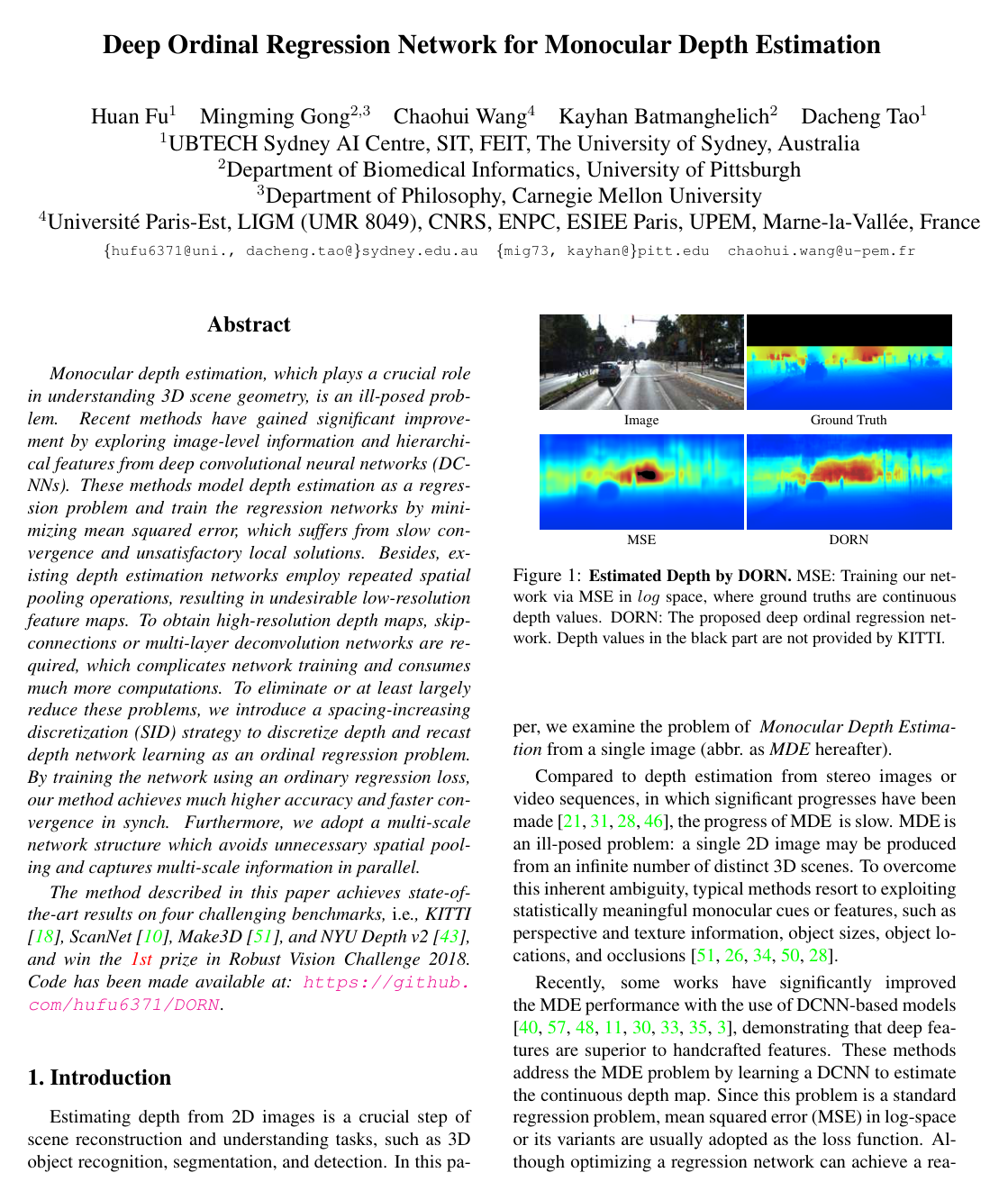
Deep Ordinal Regression Network for Monocular Depth Estimation

Huan FuMingming GongChaohui WangKayhan BatmanghelichDacheng Tao

article2018CVPR2,044 citations1st prize in Robust Vision Challenge 2018

Presents an ordinal regression framework for monocular depth estimation that combines spacing-increasing discretization with a multi-scale architecture to achieve faster training convergence and superior accuracy across major benchmarks.

Listen

Estimating three-dimensional distance from a single two-dimensional image is a critical capability for autonomous driving, robotics, and scene understanding. However, single-image depth estimation is inherently ambiguous, as many distinct physical environments can generate the exact same two-dimensional image. Conventional deep learning methods treat this challenge as a standard continuous regression task, which frequently suffers from slow training convergence and poor local solutions. Furthermore, existing architectures rely on aggressive spatial pooling that drastically degrades feature resolution, requiring complicated and computationally heavy reconstruction modules to recover fine spatial details.

The article introduces and evaluates the Deep Ordinal Regression Network to demonstrate that reframing depth prediction as an ordinal classification problempaired with an efficient, high-resolution network architecturesubstantially improves accuracy and computational efficiency over conventional regression-based systems.

To accomplish this, the authors designed a novel formulation termed spacing-increasing discretization, which divides continuous distances into discrete bins whose intervals grow larger at greater distances to reflect increasing physical measurement uncertainty. The system predicts these ordered intervals using an ordinal regression training loss that penalizes predictions increasingly as they diverge from true values. The underlying neural network eliminates resolution loss by using dilated convolutions to preserve spatial details without downsampling, incorporates parallel multi-scale feature modules, and introduces a lightweight full-image encoder. The model was trained and benchmarked across four standard indoor and outdoor datasets: KITTI, ScanNet, Make3D, and NYU Depth v2.

The findings establish that the proposed approach consistently outperforms existing methods across all evaluated benchmarks, improving accuracy metrics by approximately 5% to 30%. On the outdoor KITTI dataset, the model reduced root mean squared error from around 4.627.16 meters in baseline systems down to 2.73 meters, while achieving an accuracy rate of 93.2% within the strictest evaluation threshold. On indoor data such as NYU Depth v2, root mean squared error decreased from roughly 0.570.64 meters to 0.51 meters. The ablation analyses confirmed that spacing-increasing discretization outperforms uniform spacing and continuous regression losses, and that the proposed full-image encoder matches or exceeds traditional full-image encoders while reducing parameter requirements by over 90% (from approximately 753 million parameters to 51 million).

These results demonstrate that transforming continuous regression into an ordinal ranking framework provides superior optimization stability and faster convergence without sacrificing precision. By coupling this mathematical framing with a streamlined network architecture, vision systems can achieve sharper depth maps at significantly lower computational and memory overhead. For engineering and deployment pipelines, this reduction in complexity mitigates training risks, lowers runtime resource demands, and enhances safety in critical perception tasks such as obstacle localization.

Based on these outcomes, teams developing monocular depth perception systems should adopt ordinal regression formulations and spacing-increasing discretization strategies over standard continuous loss metrics. The article also suggests exploring alternative depth approximations and expanding the ordinal regression framework to broader dense visual prediction problems, such as surface normal estimation or semantic segmentation.

The primary limitations of this study relate to fixed discrete interval bounds and evaluation restricted to the tested benchmark environments and sensor resolutions. Nonetheless, the consistent state-of-the-art results across both indoor and outdoor datasets, as well as victory in the Robust Vision Challenge 2018, provide high confidence in the method's effectiveness.

Cover for Deep Ordinal Regression Network for Monocular Depth Estimation

Abstract

Monocular depth estimation, which plays a crucial role in understanding 3D scene geometry, is an ill-posed problem. Recent methods have gained significant improvement by exploring image-level information and hierarchical features from deep convolutional neural networks (DCNNs). These methods model depth estimation as a regression problem and train the regression networks by minimizing mean squared error, which suffers from slow convergence and unsatisfactory local solutions. Besides, existing depth estimation networks employ repeated spatial pooling operations, resulting in undesirable low-resolution feature maps. To obtain high-resolution depth maps, skip-connections or multi-layer deconvolution networks are required, which complicates network training and consumes much more computations. To eliminate or at least largely reduce these problems, we introduce a spacing-increasing discretization (SID) strategy to discretize depth and recast depth network learning as an ordinal regression problem. By training the network using an ordinary regression loss, our method achieves much higher accuracy and \dd{faster convergence in synch}. Furthermore, we adopt a multi-scale network structure which avoids unnecessary spatial pooling and captures multi-scale information in parallel.

The method described in this paper achieves state-of-the-art results on four challenging benchmarks, i.e., KITTI [17], ScanNet [9], Make3D [50], and NYU Depth v2 [42], and win the 1st prize in Robust Vision Challenge 2018. Code has been made available at: this https URL.

Table of Contents

  • 1 Introduction
  • 2 Related Work
  • 3 Method
  • 3.1 Network Architecture
  • 3.1.1 Dense Feature Extractor
  • 3.1.2 Scene Understanding Modular
  • 3.2 Spacing-Increasing Discretization
  • 3.3 Learning and Inference
  • 4 Experiments
  • 4.1 Benchmark Perfomance
  • 4.2 Ablation Studies
  • 4.2.1 Depth Discretization
  • 4.2.2 Full-image Encoder
  • 4.2.3 How Many Intervals
  • 5 Conclusion
  • 6 Acknowledgement
  • References

Knowls

  1. Knowl 1 — Spacing-Increasing Discretization (SID) for Depth Interval Quantization

    model/method

    To transform continuous monocular depth estimation into a discrete classification or ordinal regression task, a continuous depth range [α,β][\alpha, \beta] is partitioned into KK discrete intervals. In monocular depth estimation, estimation uncertainty grows as the underlying depth increases, meaning that estimation errors are naturally larger at greater distances. Spacing-Increasing Discretization (SID) discretizes the depth range uniformly in log-space, assigning wider intervals to larger depths to down-weight large-depth losses during training and prevent distant regions from dominating optimization.

    Given the original continuous depth bounds [α,β][\alpha, \beta], an offset ξ\xi is added such that the shifted lower bound is α=α+ξ=1.0\alpha^* = \alpha + \xi = 1.0 and the shifted upper bound is β=β+ξ\beta^* = \beta + \xi. The K+1K+1 boundary thresholds tit_i for i{0,1,,K}i \in \{0, 1, \dots, K\} under SID are defined by:

    ti=elog(α)+log(β/α)iKt_i = e^{\log(\alpha^*) + \frac{\log(\beta^* / \alpha^*) \cdot i}{K}}

    In contrast, Uniform Discretization (UD) divides the interval linearly without logarithmic spacing:

    ti=α+(βα)iKt_i = \alpha + \frac{(\beta - \alpha) \cdot i}{K}

    A continuous shifted depth value d=d+ξ[tk,tk+1)d^* = d + \xi \in [t_k, t_{k+1}) is assigned the discrete ordinal interval label l=k{0,1,,K1}l = k \in \{0, 1, \dots, K-1\}.

  2. Knowl 2 — Ordinal Regression Loss and Gradient Optimization for Dense Depth Estimation

    equation

    Let χRW×H×C\chi \in \mathbb{R}^{W \times H \times C} denote intermediate feature maps extracted from an input image II, where WW, HH, and CC are the spatial width, height, and channel count. The prediction layer maps χ\chi to logits YRW×H×2KY \in \mathbb{R}^{W \times H \times 2K} via parameter weight vectors Θ=(θ0,θ1,,θ2K1)\Theta = (\theta_0, \theta_1, \dots, \theta_{2K-1}) such that y(w,h,i)=θiTx(w,h)y_{(w,h,i)} = \theta_i^T x_{(w,h)} for feature vector x(w,h)χx_{(w,h)} \in \chi at spatial coordinate (w,h)(w, h).

    For each interval boundary k{0,1,,K1}k \in \{0, 1, \dots, K-1\}, the probability P(w,h)kP^k_{(w,h)} that the predicted discrete depth label l^(w,h)\hat{l}_{(w,h)} exceeds kk is computed via a two-way softmax over logit channels 2k2k and 2k+12k+1:

    P(w,h)k=P(l^(w,h)>kχ,Θ)=ey(w,h,2k+1)ey(w,h,2k)+ey(w,h,2k+1)=eθ2k+1Tx(w,h)eθ2kTx(w,h)+eθ2k+1Tx(w,h)P^k_{(w,h)} = P(\hat{l}_{(w,h)} > k \mid \chi, \Theta) = \frac{e^{y_{(w,h,2k+1)}}}{e^{y_{(w,h,2k)}} + e^{y_{(w,h,2k+1)}} = \frac{e^{\theta_{2k+1}^T x_{(w,h)}}}{e^{\theta_{2k}^T x_{(w,h)}} + e^{\theta_{2k+1}^T x_{(w,h)}}}}

    Given the ground-truth discrete label l(w,h){0,1,,K1}l_{(w,h)} \in \{0, 1, \dots, K-1\}, the pixelwise ordinal loss Ψ(w,h,χ,Θ)\Psi(w, h, \chi, \Theta) is defined as the sum of binary cross-entropy losses across all KK ordinal classifiers:

    Ψ(w,h,χ,Θ)=k=0l(w,h)1log(P(w,h)k)+k=l(w,h)K1log(1P(w,h)k)\Psi(w, h, \chi, \Theta) = \sum_{k=0}^{l_{(w,h)}-1} \log\left(P^k_{(w,h)}\right) + \sum_{k=l_{(w,h)}}^{K-1} \log\left(1 - P^k_{(w,h)}\right)

    The total training loss L(χ,Θ)\mathcal{L}(\chi, \Theta) averaged over all N=W×HN = W \times H spatial positions is:

    L(χ,Θ)=1Nw=0W1h=0H1Ψ(w,h,χ,Θ)\mathcal{L}(\chi, \Theta) = -\frac{1}{N} \sum_{w=0}^{W-1} \sum_{h=0}^{H-1} \Psi(w, h, \chi, \Theta)

    The gradients of the pixelwise loss with respect to parameters θ2k\theta_{2k} and θ2k+1\theta_{2k+1} are:

    Ψ(w,h,χ,Θ)θ2k+1=Ψ(w,h,χ,Θ)θ2k\frac{\partial \Psi(w, h, \chi, \Theta)}{\partial \theta_{2k+1}} = -\frac{\partial \Psi(w, h, \chi, \Theta)}{\partial \theta_{2k}}

    Ψ(w,h,χ,Θ)θ2k=x(w,h)η(l(w,h)>k)(P(w,h)k1)+x(w,h)η(l(w,h)k)P(w,h)k\frac{\partial \Psi(w, h, \chi, \Theta)}{\partial \theta_{2k}} = x_{(w,h)} \eta\left(l_{(w,h)} > k\right)\left(P^k_{(w,h)} - 1\right) + x_{(w,h)} \eta\left(l_{(w,h)} \le k\right) P^k_{(w,h)}

    where η()\eta(\cdot) is an indicator function returning 11 if its boolean argument is true and 00 otherwise.

  3. Knowl 3 — Continuous Depth Decoding from Ordinal Predictions

    equation

    Given predicted binary ordinal probabilities P(w,h)k=P(l^(w,h)>kχ,Θ)P^k_{(w,h)} = P(\hat{l}_{(w,h)} > k \mid \chi, \Theta) for all ordinal thresholds k{0,1,,K1}k \in \{0, 1, \dots, K-1\} at spatial coordinate (w,h)(w, h), the discrete depth index l^(w,h)\hat{l}_{(w,h)} is decoded by counting the number of ordinal classifiers whose predicted probability is at least 0.50.5:

    l^(w,h)=k=0K1η(P(w,h)k0.5)\hat{l}_{(w,h)} = \sum_{k=0}^{K-1} \eta\left(P^k_{(w,h)} \ge 0.5\right)

    where η()\eta(\cdot) is the indicator function (η(true)=1,η(false)=0 \eta(\text{true})=1, \eta(\text{false})=0).

    The continuous depth estimate d^(w,h)\hat{d}_{(w,h)} is reconstructed from the predicted discrete interval index l^(w,h)\hat{l}_{(w,h)} as the midpoint of the sub-interval [tl^(w,h),tl^(w,h)+1)[t_{\hat{l}_{(w,h)}}, t_{\hat{l}_{(w,h)}+1}), corrected by subtracting the discretization shift ξ\xi:

    d^(w,h)=tl^(w,h)+tl^(w,h)+12ξ\hat{d}_{(w,h)} = \frac{t_{\hat{l}_{(w,h)}} + t_{\hat{l}_{(w,h)}+1}}{2} - \xi

    where tit_i are the Spacing-Increasing Discretization thresholds.

  4. Knowl 4 — Deep Ordinal Regression Network (DORN) Architecture

    model/method

    The Deep Ordinal Regression Network (DORN) for monocular depth estimation avoids multi-scale stage-wise networks and deconvolutional decoding stacks by combining a dilated dense feature extractor with a multi-branch scene understanding module:

    1. Dense Feature Extractor: A CNN backbone (e.g., ResNet-101 or VGG-16) modified by removing the downsampling (striding/max-pooling) operations in the final pooling layers and applying dilated (atrous) convolutions in subsequent convolutional layers. This retains a higher spatial resolution (stride 8 relative to input) while maintaining large receptive fields without increasing parameter count.

    2. Scene Understanding Module: Operating on the dense feature map FRC×h×w\mathcal{F} \in \mathbb{R}^{C \times h \times w}, the module runs three parallel components:

      • Atrous Spatial Pyramid Pooling (ASPP): Three parallel 3×33 \times 3 dilated convolutional layers with dilation rates of 6, 12, and 18 to capture multi-scale context.
      • Cross-Channel Learner: A 1×11 \times 1 convolutional layer to capture cross-channel interactions.
      • Full-Image Context Encoder: A parameter-efficient module that compresses global features and broadcasts them spatially across the map.
    3. Prediction Layer: The feature outputs from all three components are concatenated along channels. A 1×11 \times 1 convolutional layer reduces channel dimension and learns cross-branch interactions, followed by a final 1×11 \times 1 convolutional layer that outputs 2K2K channels corresponding to the logits for the KK binary ordinal classifiers.

  5. Knowl 5 — Parameter-Efficient Full-Image Context Encoder

    model/method

    In monocular depth estimation, global image context resolves local depth ambiguities. Traditional full-image encoders use fully connected (fcfc) layers that connect every location of feature map FRC×h×w\mathcal{F} \in \mathbb{R}^{C \times h \times w} to an intermediate vector of size mm, and then map back to C×h×wC \times h \times w, requiring approximately 1s2mwhC+m2+1s2whCm\frac{1}{s^2} m w h C + m^2 + \frac{1}{s^2} w h C m parameters (where ss is an additional spatial downsampling stride). For C=512,m=2048,h=49,w=65,s=3C=512, m=2048, h=49, w=65, s=3, this consumes 753M\approx 753\text{M} parameters.

    The parameter-efficient full-image context encoder reduces parameter count through the following pipeline:

    1. An average pooling layer with small kernel size and stride k×kk \times k (e.g., k=4k=4) reduces F\mathcal{F} to spatial size (h/k)×(w/k)(h/k) \times (w/k).
    2. A fully connected layer maps the pooled features to a CC-dimensional vector.
    3. A 1×11 \times 1 convolutional layer acts as a cross-channel parametric pooling structure on the C×1×1C \times 1 \times 1 representation.
    4. The resulting CC-dimensional vector is copied/broadcast across spatial dimensions h×wh \times w to form global feature tensor FˉRC×h×w\bar{\mathcal{F}} \in \mathbb{R}^{C \times h \times w}.

    This design requires Cw4h4C+CC51MC \cdot \frac{w}{4} \cdot \frac{h}{4} \cdot C + C \cdot C \approx 51\text{M} parameters (a >93%>93\% parameter reduction) while achieving slightly higher accuracy (threshold accuracy δ<1.25\delta < 1.25 of 0.9150.915 vs. 0.9100.910 for the fcfc-based encoder on KITTI).

  6. Knowl 6 — Ablation Study: Loss Formulations, Discretization Strategies, and Full-Image Encoders

    data/table

    Ablation experiments evaluated on the KITTI dataset (Eigen test split, depth cap 080m0-80\text{m}) compare continuous regression losses, multi-class classification (MCC), and deep ordinal regression network (DORN) losses under Uniform Discretization (UD) and Spacing-Increasing Discretization (SID), alongside encoder architectural variants.

    Variant Iterations δ<1.25\delta < 1.25 δ<1.252\delta < 1.25^2 δ<1.253\delta < 1.25^3 Abs Rel Squa Rel RMSE RMSElog\text{RMSE}_{\log}
    MSE 1.0M 0.864 0.969 0.991 0.109 0.527 3.660 0.164
    MSE-SID 0.6M 0.865 0.970 0.992 0.108 0.520 3.636 0.163
    MCC-UD 0.3M 0.892 0.970 0.988 0.093 0.474 3.438 0.155
    MCC-SID 0.3M 0.906 0.976 0.991 0.084 0.417 3.201 0.142
    DORN-UD 0.3M 0.900 0.973 0.991 0.091 0.452 3.339 0.148
    DORN-SID 0.3M 0.915 0.980 0.993 0.081 0.376 3.056 0.132
    berHu (ResNet) 0.6M 0.909 0.978 0.992 0.086 0.385 3.365 0.136
    DORN-SID (ResNet) 0.3M 0.932 0.984 0.994 0.072 0.307 2.727 0.120
    Full-Image Encoder Variant δ<1.25\delta < 1.25 Abs Rel RMSElog\text{RMSE}_{\log} Params
    Without full-image encoder 0.906 0.092 0.143 0M
    FC-fashion encoder 0.910 0.085 0.137 753M
    Proposed encoder 0.915 0.081 0.132 51M

    The data shows:

    1. Discretizing continuous depth into ordinal sub-intervals (DORN-SID) converges faster (0.3M0.3\text{M} iterations vs. 1.0M1.0\text{M} for MSE) and improves accuracy from δ<1.25=0.864\delta < 1.25 = 0.864 to 0.9150.915 on VGG-16 and 0.9320.932 on ResNet-101.
    2. SID consistently outperforms UD across classification (MCC) and ordinal regression (DORN).
    3. Ordinal regression loss outperforms multi-class classification loss by penalizing predictions according to their distance from the true label.
    4. The proposed full-image encoder matches or exceeds the accuracy of dense fcfc encoders while using 14.7×\approx 14.7\times fewer parameters.
  7. Knowl 7 — Monocular Depth Estimation Performance on KITTI Benchmark

    data/table

    Evaluation on the KITTI outdoor dataset using the standard Eigen test split (697 test images from 29 scenes, depth ranges 080m0-80\text{m} and 050m0-50\text{m}) and the online KITTI test server.

    Method Depth Cap δ<1.25\delta < 1.25 δ<1.252\delta < 1.25^2 δ<1.253\delta < 1.25^3 Abs Rel Squa Rel RMSE RMSElog\text{RMSE}_{\log}
    Make3D (Saxena et al.) 080m0-80\text{m} 0.601 0.820 0.926 0.280 3.012 8.734 0.361
    Eigen et al. 080m0-80\text{m} 0.692 0.899 0.967 0.190 1.515 7.156 0.270
    Liu et al. 080m0-80\text{m} 0.647 0.882 0.961 0.217 1.841 6.986 0.289
    LRC (CS + K) (Godard et al.) 080m0-80\text{m} 0.861 0.949 0.976 0.114 0.898 4.935 0.206
    Kuznietsov et al. 080m0-80\text{m} 0.862 0.960 0.986 0.113 0.741 4.621 0.189
    DORN (VGG) 080m0-80\text{m} 0.915 0.980 0.993 0.081 0.376 3.056 0.132
    DORN (ResNet) 080m0-80\text{m} 0.932 0.984 0.994 0.072 0.307 2.727 0.120
    Garg et al. 050m0-50\text{m} 0.740 0.904 0.962 0.169 1.080 5.104 0.273
    LRC (CS + K) (Godard et al.) 050m0-50\text{m} 0.873 0.954 0.979 0.108 0.657 3.729 0.194
    Kuznietsov et al. 050m0-50\text{m} 0.875 0.964 0.988 0.108 0.595 3.518 0.179
    DORN (VGG) 050m0-50\text{m} 0.920 0.982 0.994 0.079 0.324 2.517 0.128
    DORN (ResNet) 050m0-50\text{m} 0.936 0.985 0.995 0.071 0.268 2.271 0.116
    Method (KITTI Online Server) SILog sqErrorRel absErrorRel iRMSE
    Official Baseline 18.19 7.32 14.24 18.50
    DORN 11.77 2.23 8.78 12.98

    DORN (ResNet) reduces RMSE from 4.6214.621 to 2.7272.727 (>40%>40\% reduction) and improves the δ<1.25\delta < 1.25 threshold metric from 0.8620.862 to 0.9320.932 on the 080m0-80\text{m} benchmark compared to previous state of the art.

  8. Knowl 8 — Monocular Depth Estimation Performance on NYU Depth v2, Make3D, and ScanNet

    data/table

    Performance comparison across indoor (NYU Depth v2, ScanNet) and outdoor (Make3D) datasets.

    Method (NYU Depth v2) δ<1.25\delta < 1.25 δ<1.252\delta < 1.25^2 δ<1.253\delta < 1.25^3 Rel log10\log_{10} RMS
    Make3D (Saxena et al.) 0.447 0.745 0.897 0.349 - 1.214
    DepthTransfer (Karsch et al.) - - - 0.35 0.131 1.2
    Liu et al. - - - 0.335 0.127 1.06
    Ladicky et al. 0.542 0.829 0.941 - - -
    Li et al. 0.621 0.886 0.968 0.232 0.094 0.821
    Wang et al. 0.605 0.890 0.970 0.220 - 0.824
    Roy et al. - - - 0.187 - 0.744
    Liu et al. 0.650 0.906 0.976 0.213 0.087 0.759
    Eigen et al. 0.769 0.950 0.988 0.158 - 0.641
    Chakrabarti et al. 0.806 0.958 0.987 0.149 - 0.620
    Laina et al. (ResNet) 0.811 0.953 0.988 0.127 0.055 0.573
    Li et al. (ResNet) 0.788 0.958 0.991 0.143 0.063 0.635
    MS-CRF (Xu et al., ResNet) 0.811 0.954 0.987 0.121 0.052 0.586
    DORN (ResNet) 0.828 0.965 0.992 0.115 0.051 0.509
    Method (Make3D) C1 rel C1 log10\log_{10} C1 rms C2 rel C2 log10\log_{10} C2 rms
    DepthTransfer (Karsch et al.) 0.355 0.127 9.20 0.361 0.148 15.10
    Liu et al. 0.287 0.109 7.36 0.287 0.122 14.09
    Laina et al. 0.176 0.072 4.46 - - -
    MS-CRF (Xu et al.) 0.184 0.065 4.38 0.198 - 8.56
    DORN (VGG) 0.236 0.082 7.02 0.238 0.087 10.01
    DORN (ResNet) 0.157 0.062 3.97 0.162 0.067 7.32
    ScanNet Server abs rel imae irmse log mae log rmse mae rmse scale invar. sq. rel
    Official Baseline 0.25 0.17 0.21 0.24 0.29 0.42 0.53 0.05 0.14
    DORN 0.14 0.10 0.13 0.13 0.17 0.22 0.29 0.02 0.06

    On NYU Depth v2, DORN achieves RMS=0.509\text{RMS} = 0.509 and δ<1.25=0.828\delta < 1.25 = 0.828. On Make3D, DORN achieves C1 relative error of 0.1570.157 and RMS of 3.97m3.97\text{m}. On the online ScanNet test server, DORN reduces absolute relative error from 0.250.25 to 0.140.14 and RMSE from 0.530.53 to 0.290.29.

  9. Knowl 9 — Sensitivity of Monocular Depth Estimation to Discretization Interval Count

    empirical result

    When depth is discretized using Spacing-Increasing Discretization (SID), the performance of DORN remains stable across a wide range of interval counts KK.

    Evaluating interval counts KK from 4040 to 120120 on KITTI shows that the accuracy metric δ<1.25\delta < 1.25 remains within [0.908,0.915][0.908, 0.915] and the RMSE metric remains within [3.056,3.125][3.056, 3.125].

    Performance degrades at the extremes:

    • Too few intervals (K<40K < 40) leads to large quantization errors due to overly coarse bin widths.
    • Too many intervals (K>120K > 120) causes the network to lose the convergence advantages of discretization by increasing classification difficulty.

Coverage note — No substantial contributed material was omitted.

References

  1. 1.M. H. Baig and L. Torresani. Coupled depth learning. In WACV, 2016. 2
  2. 2.A. Chakrabarti, J. Shao, and G. Shakhnarovich. Depth from a single image by harmonizing overcomplete local network predictions. In NIPS, 2016. 2, 3, 4, 7
  3. 3.A. Chang, A. Dai, T. Funkhouser, M. Halber, M. Niessner, M. Savva, S. Song, A. Zeng, and Y. Zhang. Matterport3D: Learning from RGB-D data in indoor environments. 3DV, 2017. 1
  4. 4.L.-C. Chen, G. Papandreou, I. Kokkinos, K. Murphy, and A. L. Yuille. Semantic image segmentation with deep convolutional nets and fully connected crfs. In ICLR, 2015. 2, 3
  5. 5.L.-C. Chen, G. Papandreou, I. Kokkinos, K. Murphy, and A. L. Yuille. Deeplab: Semantic image segmentation with deep convolutional nets, atrous convolution, and fully connected crfs. arXiv:1606.00915, 2016. 3
  6. 6.L.-C. Chen, G. Papandreou, F. Schroff, and H. Adam. Rethinking atrous convolution for semantic image segmentation. arXiv preprint arXiv:1706.05587, 2017. 2, 3
  7. 7.W. Chen, Z. Fu, D. Yang, and J. Deng. Single-image depth perception in the wild. In NIPS, 2016. 3
  8. 8.S. Choi, D. Min, B. Ham, Y. Kim, C. Oh, and K. Sohn. Depth analogy: Data-driven approach for single image depth estimation using gradient samples. IEEE TIP, 24(12):5953–5966, 2015. 2
  9. 9.K. Crammer and Y. Singer. Pranking with ranking. In NIPS, 2002. 3
  10. 10.A. Dai, A. X. Chang, M. Savva, M. Halber, T. Funkhouser, and M. Nießner. Scannet: Richly-annotated 3d reconstructions of indoor scenes. In CVPR, 2017. 1, 2, 6
  11. 11.D. Eigen and R. Fergus. Predicting depth, surface normals and semantic labels with a common multi-scale convolutional architecture. In ICCV, 2015. 1, 2, 3, 4, 7, 8
  12. 12.D. Eigen, C. Puhrsch, and R. Fergus. Depth map prediction from a single image using a multi-scale deep network. In NIPS, 2014. 2, 3, 4, 5, 6, 7, 8
  13. 13.J. Flynn, I. Neulander, J. Philbin, and N. Snavely. Deepstereo: Learning to predict new views from the world’s imagery. In CVPR, 2016. 2
  14. 14.D. Forsyth and J. Ponce. Computer Vision: a Modern Approach. Prentice Hall, 2002. 2
  15. 15.E. Frank and M. Hall. A simple approach to ordinal classification. ECML, 2001. 3
  16. 16.R. Furukawa, R. Sagawa, and H. Kawasaki. Depth estimation using structured light flow – analysis of projected pattern flow on an object’s surface. In ICCV, 2017. 2
  17. 17.R. Garg, G. Carneiro, and I. Reid. Unsupervised cnn for single view depth estimation: Geometry to the rescue. In ECCV, 2016. 2, 3, 7
  18. 18.A. Geiger, P. Lenz, C. Stiller, and R. Urtasun. Vision meets robotics: The kitti dataset. IJRR, 2013. 1, 2, 5
  19. 19.C. Godard, O. Mac Aodha, and G. J. Brostow. Unsupervised monocular depth estimation with left-right consistency. CVPR, 2017. 5, 7
  20. 20.R. A. Guler, G. Trigeorgis, E. Antonakos, P. Snape, ¨ S. Zafeiriou, and I. Kokkinos. Densereg: Fully convolutional dense shape regression in-the-wild. In CVPR, 2016. 2
  21. 21.H. Ha, S. Im, J. Park, H.-G. Jeon, and I. S. Kweon. Highquality depth from uncalibrated small motion clip. In CVPR, 2016. 1
  22. 22.C. Hane, L. Ladicky, and M. Pollefeys. Direction matters: Depth estimation with a surface normal classifier. In CVPR, 2015. 2
  23. 23.F. E. Harrell Jr. Regression modeling strategies: with applications to linear models, logistic and ordinal regression, and survival analysis. Springer, 2015. 3
  24. 24.K. He, X. Zhang, S. Ren, and J. Sun. Deep residual learning for image recognition. In CVPR, 2016. 2, 5
  25. 25.R. Herbrich, T. Graepel, and K. Obermayer. Support vector learning for ordinal regression. 1999. 3
  26. 26.D. Hoiem, A. A. Efros, and M. Hebert. Recovering surface layout from an image. IJCV, 75(1):151–172, 2007. 1, 2
  27. 27.Y. Jia, E. Shelhamer, J. Donahue, S. Karayev, J. Long, R. Girshick, S. Guadarrama, and T. Darrell. Caffe: Convolutional architecture for fast feature embedding. arXiv preprint arXiv:1408.5093, 2014. 5
  28. 28.K. Karsch, C. Liu, and S. B. Kang. Depth transfer: Depth extraction from video using non-parametric sampling. IEEE TPAMI, 36(11):2144–2158, 2014. 1, 2, 6, 7
  29. 29.A. Kendall and Y. Gal. What uncertainties do we need in bayesian deep learning for computer vision? In NIPS, 2017. 2
  30. 30.S. Kim, K. Park, K. Sohn, and S. Lin. Unified depth prediction and intrinsic image decomposition from a single image via joint convolutional neural fields. In ECCV, 2016. 1, 2, 7
  31. 31.N. Kong and M. J. Black. Intrinsic depth: Improving depth transfer with intrinsic images. In ICCV, 2015. 1
  32. 32.J. Konrad, M. Wang, P. Ishwar, C. Wu, and D. Mukherjee. Learning-based, automatic 2d-to-3d image and video conversion. IEEE TIP, 22(9):3485–3496, 2013. 2
  33. 33.Y. Kuznietsov, J. Stuckler, and B. Leibe. Semi-supervised ¨ deep learning for monocular depth map prediction. CVPR, 2017. 1, 2, 3, 7
  34. 34.L. Ladicky, J. Shi, and M. Pollefeys. Pulling things out of perspective. In CVPR, 2014. 1, 2, 7
  35. 35.I. Laina, C. Rupprecht, V. Belagiannis, F. Tombari, and N. Navab. Deeper depth prediction with fully convolutional residual networks. In 3DV, 2016. 1, 2, 3, 7
  36. 36.B. Li, C. Shen, Y. Dai, A. van den Hengel, and M. He. Depth and surface normal estimation from monocular images using regression on deep features and hierarchical crfs. In CVPR, 2015. 7
  37. 37.J. Li, R. Klein, and A. Yao. A two-streamed network for estimating fine-scaled depth maps from single rgb images. In ICCV, 2017. 2, 7
  38. 38.X. Li, H. Qin, Y. Wang, Y. Zhang, and Q. Dai. Dept: depth estimation by parameter transfer for single still images. In ACCV, 2014. 2
  39. 39.B. Liu, S. Gould, and D. Koller. Single image depth estimation from predicted semantic labels. In CVPR, 2010. 7
  40. 40.F. Liu, C. Shen, G. Lin, and I. Reid. Learning depth from single monocular images using deep convolutional neural fields. IEEE TPAMI, 38(10):2024–2039, 2016. 1, 2, 3, 5, 6, 7
  41. 41.M. Liu, M. Salzmann, and X. He. Discrete-continuous depth estimation from a single image. In CVPR, 2014. 2, 7
  42. 42.T. Narihira, M. Maire, and S. X. Yu. Learning lightness from human judgement on relative reflectance. In CVPR, 2015. 2
  43. 43.P. K. Nathan Silberman, Derek Hoiem and R. Fergus. Indoor segmentation and support inference from rgbd images. In ECCV, 2012. 1, 2, 5, 6
  44. 44.Z. Niu, M. Zhou, L. Wang, X. Gao, and G. Hua. Ordinal regression with multiple output cnn for age estimation. In CVPR, 2016. 3
  45. 45.A. Oliva and A. Torralba. Modeling the shape of the scene: A holistic representation of the spatial envelope. IJCV, 42(3):145–175, 2001. 2
  46. 46.A. Rajagopalan, S. Chaudhuri, and U. Mudenagudi. Depth estimation and image restoration using defocused stereo pairs. IEEE TPAMI, 26(11):1521–1525, 2004. 1
  47. 47.R. Ranftl, V. Vineet, Q. Chen, and V. Koltun. Dense monocular depth estimation in complex dynamic scenes. In CVPR, 2016. 2
  48. 48.A. Roy and S. Todorovic. Monocular depth estimation using neural regression forest. In CVPR, 2016. 1, 2, 7
  49. 49.O. Russakovsky, J. Deng, H. Su, J. Krause, S. Satheesh, S. Ma, Z. Huang, A. Karpathy, A. Khosla, M. Bernstein, A. C. Berg, and L. Fei-Fei. ImageNet Large Scale Visual Recognition Challenge. IJCV, 115(3):211–252, 2015. 5
  50. 50.A. Saxena, S. H. Chung, and A. Y. Ng. Learning depth from single monocular images. In NIPS, 2006. 1, 2, 5, 6
  51. 51.A. Saxena, M. Sun, and A. Y. Ng. Make3d: Learning 3d scene structure from a single still image. IEEE TPAMI, 31(5):824–840, 2009. 1, 2, 5, 6, 7
  52. 52.D. Scharstein and R. Szeliski. A taxonomy and evaluation of dense two-frame stereo correspondence algorithms. IJCV, 47(1-3):7–42, 2002. 2
  53. 53.A. Shashua and A. Levin. Ranking with large margin principle: Two approaches. In NIPS, 2003. 3
  54. 54.E. Shelhamer, J. T. Barron, and T. Darrell. Scene intrinsics and depth from a single image. In ICCV Workshop, 2015. 2
  55. 55.J. Shi, X. Tao, L. Xu, and J. Jia. Break ames room illusion: depth from general single images. ACM TOG, 34(6):225, 2015. 2
  56. 56.K. Simonyan and A. Zisserman. Very deep convolutional networks for large-scale image recognition. In ICLR, 2015. 2, 5
  57. 57.P. Wang, X. Shen, Z. Lin, S. Cohen, B. Price, and A. Yuille. Towards unified depth and semantic prediction from a single image. In CVPR, 2015. 1, 2, 4, 7
  58. 58.X. Wang, D. Fouhey, and A. Gupta. Designing deep networks for surface normal estimation. In CVPR, 2015. 2
  59. 59.J. Xie, R. Girshick, and A. Farhadi. Deep3d: Fully automatic 2d-to-3d video conversion with deep convolutional neural networks. In ECCV, 2016. 2, 3, 7
  60. 60.D. Xu, E. Ricci, W. Ouyang, X. Wang, and N. Sebe. Multiscale continuous crfs as sequential deep networks for monocular depth estimation. In CVPR, 2017. 7
  61. 61.X. You, Q. Li, D. Tao, W. Ou, and M. Gong. Local metric learning for exemplar-based object detection. IEEE TCSVT, 24(8):1265–1276, 2014. 2
  62. 62.F. Yu and V. Koltun. Multi-scale context aggregation by dilated convolutions. In ICLR, 2016. 2, 3
  63. 63.Z. Zhang, A. G. Schwing, S. Fidler, and R. Urtasun. Monocular object instance segmentation and depth ordering with cnns. In ICCV, 2015. 2
  64. 64.H. Zhao, J. Shi, X. Qi, X. Wang, and J. Jia. Pyramid scene parsing network. In CVPR, 2017. 2, 3
  65. 65.W. Zhuo, M. Salzmann, X. He, and M. Liu. Indoor scene structure analysis for single image depth estimation. In CVPR, 2015. 2
  66. 66.D. Zoran, P. Isola, D. Krishnan, and W. T. Freeman. Learning ordinal relationships for mid-level vision. In ICCV, 2015. 3

Citation

MLA
Fu, H., et al. “Deep Ordinal Regression Network for Monocular Depth Estimation”. arXiv, 2018, http://arxiv.org/abs/1806.02446v1.
APA
Fu, H., Gong, M., Wang, C., Batmanghelich, K., & Tao, D. (2018). Deep Ordinal Regression Network for Monocular Depth Estimation. arXiv. http://arxiv.org/abs/1806.02446v1
Chicago
Fu, H., M. Gong, C. Wang, K. Batmanghelich, and D. Tao. 2018. “Deep Ordinal Regression Network for Monocular Depth Estimation”. arXiv. http://arxiv.org/abs/1806.02446v1.
Harvard
Fu, H. et al. (2018) “Deep Ordinal Regression Network for Monocular Depth Estimation”, arXiv [Preprint]. Available at: http://arxiv.org/abs/1806.02446v1.
Vancouver
1. Fu H, Gong M, Wang C, Batmanghelich K, Tao D (2018) Deep Ordinal Regression Network for Monocular Depth Estimation. arXiv

BibTeX

@article{fu2018deep,
  title = {Deep Ordinal Regression Network for Monocular Depth Estimation},
  author = {Fu, Huan and Gong, Mingming and Wang, Chaohui and Batmanghelich, Kayhan and Tao, Dacheng},
  year = {2018},
  journal = {arXiv},
  url = {http://arxiv.org/abs/1806.02446v1},
  eprint = {1806.02446}
}
Metadata:arXiv

Source Code

This paper has an official code repository available. Click below to access the source code.

View Repository

Access the Paper

This paper is available from its original source. Click below to access the PDF.

Open PDF

License: IEEE