
Domain Separation Networks
Konstantinos Bousmalis$^{*}$
Google Brain
Mountain View, CA
[email protected]
George Trigeorgis$^{*}$ $^{\dagger}$
Imperial College London
London, UK
[email protected]
Nathan Silberman
Google Research
New York, NY
[email protected]
Dilip Krishnan
Google Research
Cambridge, MA
[email protected]
Dumitru Erhan
Google Brain
Mountain View, CA
[email protected]
$^{*}$ Authors contributed equally.
$^{\dagger}$ This work was completed while George Trigeorgis was at Google Brain in Mountain View, CA.
Abstract
The cost of large scale data collection and annotation often makes the application of machine learning algorithms to new tasks or datasets prohibitively expensive. One approach circumventing this cost is training models on synthetic data where annotations are provided automatically. Despite their appeal, such models often fail to generalize from synthetic to real images, necessitating domain adaptation algorithms to manipulate these models before they can be successfully applied. Existing approaches focus either on mapping representations from one domain to the other, or on learning to extract features that are invariant to the domain from which they were extracted. However, by focusing only on creating a mapping or shared representation between the two domains, they ignore the individual characteristics of each domain. We suggest that explicitly modeling what is unique to each domain can improve a model's ability to extract domain-invariant features. Inspired by work on private-shared component analysis, we explicitly learn to extract image representations that are partitioned into two subspaces: one component which is private to each domain and one which is shared across domains. Our model is trained not only to perform the task we care about in the source domain, but also to use the partitioned representation to reconstruct the images from both domains. Our novel architecture results in a model that outperforms the state-of-the-art on a range of unsupervised domain adaptation scenarios and additionally produces visualizations of the private and shared representations enabling interpretation of the domain adaptation process.
Executive Summary: Collecting and manually annotating large-scale datasets for machine learning is costly and time-consuming. While generating synthetic computer imagery offers an inexpensive alternative with limitless labeled data, models trained on synthetic data typically struggle to generalize to real-world target environments due to discrepancies in background, lighting, and noise. Standard domain adaptation methods attempt to overcome this by learning shared representations across domains or mapping source features to the target, but they often allow domain-specific noise to contaminate the shared features, degrading final model accuracy.
The main objective of the article is to demonstrate that explicitly isolating domain-specific characteristics into a private subspace while simultaneously learning a clean, shared subspace across domains significantly improves cross-domain model generalization.
To accomplish this, the authors introduce Domain Separation Networks. The architecture separates image features into two distinct parts: a shared component common to both source and target data, and private components unique to each specific domain. The framework enforces this separation using a similarity loss to align shared features, a difference loss to keep private and shared representations distinct, and an image reconstruction step to ensure no critical structural information is lost. The authors evaluated this approach across standard image classification benchmarks—such as synthetic digit recognition transferred to real street house numbers and synthetic traffic signs transferred to real images—as well as a synthetic-to-real three-dimensional object pose estimation task.
The evaluation produced several key findings. First, the proposed method consistently established new state-of-the-art results across all evaluated domain adaptation scenarios. For instance, when transferring from Street View House Numbers to standard digit recognition, accuracy rose to 82.7%, outperforming the leading baseline at 70.7%. Second, in realistic three-dimensional object recognition and pose estimation, the architecture achieved 100% classification accuracy and reduced the average rotational pose error to 53.3 degrees, improving upon competing methods. Third, ablation tests demonstrated that removing the difference loss or using standard reconstruction metrics consistently degraded performance, confirming that explicit subspace partitioning is essential. Finally, decoding the isolated components provided clear visual interpretations, verifying that the shared encoder effectively captures the core object while the private encoders isolate domain-specific background textures and lighting.
These results demonstrate that organizations can significantly lower data curation costs by training machine learning models on synthetic data without suffering severe drops in real-world performance. By actively separating irrelevant domain noise rather than merely forcing all features to align, the network produces more robust and interpretable models, lowering deployment risks in computer vision applications.
Organizations developing vision systems should consider adopting partitioned feature architectures when leveraging synthetic pipelines. While the method delivers strong results, the authors acknowledge that tuning model parameters currently requires a small validation set of labeled target data, as fully unsupervised parameter selection remains an unresolved challenge. Consequently, future work should prioritize establishing reliable, unsupervised hyperparameter tuning methods and extending the architecture to handle severe variations in high-level object geometry.
1. Introduction
Section Summary: The success of modern supervised learning depends on massive labeled datasets, which are costly to create in the real world, yet models trained on cheap synthetic images typically fail to work on realistic photos. This paper tackles the resulting domain adaptation problem, where a labeled source domain must be used to learn task-relevant features that also apply to an unlabeled target domain whose low-level image statistics differ. To do so, the authors introduce Domain Separation Networks that explicitly split each image’s representation into a private subspace capturing domain-specific details and a shared subspace that is forced to be task-relevant and invariant across domains.
The recent success of supervised learning algorithms has been partially attributed to the large-scale datasets [1, 2] on which they are trained. Unfortunately, collecting, annotating, and curating such datasets is an extremely expensive and time-consuming process. An alternative would be creating large-scale datasets in non–realistic but inexpensive settings, such as computer generated scenes. While such approaches offer the promise of effectively unlimited amounts of labeled data, models trained in such settings do not generalize well to realistic domains. Motivated by this, we examine the problem of learning representations that are domain–invariant in scenarios where the data distributions during training and testing are different. In this setting, the source data is labeled for a particular task and we would like to transfer knowledge from the source to the target domain for which we have no ground truth labels.
In this work, we focus on the tasks of object classification and pose estimation, where the object of interest is in the foreground of a given image, for both source and target domains. The source and target pixel distributions can differ in a number of ways. We define "low-level" differences in the distributions as those arising due to noise, resolution, illumination and color. "High-level" differences relate to the number of classes, the types of objects, and geometric variations, such as 3D position and pose. We assume that our source and target domains differ mainly in terms of the distribution of low level image statistics and that they have high level parameters with similar distributions and the same label space.
We propose a novel method, the Domain Separation Networks (DSN), for learning domain–invariant representations. Previous work attempts to either find a mapping from representations of the source domain to those of the target [3], or find representations that are shared between the two domains [4, 5, 6]. While this, in principle, is a good idea, it leaves the shared representations vulnerable to contamination by noise that is correlated with the underlying shared distribution [7]. Our model, in contrast, introduces the notion of a private subspace for each domain, which captures domain specific properties, such as background and low level image statistics. A shared subspace, enforced through the use of autoencoders and explicit loss functions, captures representations shared by the domains. By finding a shared subspace that is orthogonal to the subspaces that are private, our model is able to separate the information that is unique to each domain, and in the process produce representations that are more more meaningful for the task at hand. Our method outperforms the state–of–the–art domain adaptation techniques on a range of datasets for object classification and pose estimation, while having an interpretability advantage by allowing the visualization of these private and shared representations. In Section 2, we survey related work and introduce relevant terminology. Our architecture, loss functions and learning regime are presented in Section 3. Experimental results and discussion are given in Section 4. Finally, conclusions and directions for future work are in Section 5.
2. Related Work
Section Summary: Researchers have developed several techniques to adapt convolutional neural networks so they can perform well on a new target dataset without labeled examples from that set. Early theoretical work established bounds on adaptation performance and showed how to use a separate classifier that tries to tell the source and target data apart. Building on this idea, later methods either train networks to fool such a domain classifier through adversarial training, minimize a statistical distance called MMD between the two domains, or learn a simple transformation that aligns the statistical properties of features from each domain.
Learning to perform unsupervised domain adaptation is an open theoretical and practical problem. While much prior art exists, our literature review focuses primarily on Convolutional Neural Network (CNN) based methods due to their empirical superiority on this problem [4, 6, 3, 8]. Ben-David et al. [9] provide upper bounds on a domain-adapted classifier in the target domain. They introduce the idea of training a binary classifier trained to distinguish source and target domains. The error that this "domain incoherence" classifier provides (along with the error of a source domain specific classifier) combine to give the overall bounds. Mansour et al. [10] extend the theory of [9] to handle the case of multiple source domains.
Ganin et al. [11, 4] and Ajakan et al. [12] use adversarial training to find domain–invariant representations in-network. Their Domain–Adversarial Neural Networks (DANN) exhibit an architecture whose first few feature extraction layers are shared by two classifiers trained simultaneously. The first is trained to correctly predict task-specific class labels on the source data while the second is trained to predict the domain of each input. DANN minimizes the domain classification loss with respect to parameters specific to the domain classifier, while maximizing it with respect to the parameters that are common to both classifiers. This minimax optimization becomes possible via the use of a gradient reversal layer (GRL).
Tzeng et al. [8] and Long et al. [6] proposed versions of this model where the maximization of the domain classification loss is replaced by the minimization of the Maximum Mean Discrepancy (MMD) metric [13]. The MMD metric is computed between features extracted from sets of samples from each domain. The Deep Domain Confusion Network by Tzeng et al. [8] has an MMD loss at one layer in the CNN architecture while Long et al. [6] proposed the Deep Adaptation Network that has MMD losses at multiple layers.
Other related techniques involve learning a transformation from one domain to the other. In this setup, the feature extraction pipeline is fixed during the domain adaptation optimization. This has been applied in various non-CNN based approaches [14, 15, 16] as well as the recent CNN-based Correlation Alignment (CORAL) [3] algorithm which "recolors" whitened source features with the covariance of features from the target domain.
3. Method
Section Summary: Domain Separation Networks aim to improve image classification across different domains by training a model on labeled source data that generalizes to unlabeled target data. They achieve this by using separate encoders to extract both shared features common to both domains and private features unique to each, then combining those representations in a decoder to reconstruct the original images. Training minimizes a joint loss that enforces similarity in the shared features, orthogonality between shared and private ones, accurate classification on the source domain, and faithful reconstruction, so that the final classifier operates only on clean, domain-invariant inputs.
While the Domain Separation Networks (DSNs) could in principle be applicable to other learning tasks, without loss of generalization, we mainly use image classification as the cross-domain task. Given a labeled dataset in a source domain and an unlabeled dataset in a target domain, our goal is to train a classifier on data from the source domain that generalizes to the target domain. Like previous efforts [11, 4], our model is trained such that the representations of images from the source domain are similar to those from the target domain. This allows a classifier trained on images from the source domain to generalize as the inputs to the classifier are in theory invariant to the domain of origin. However, these representations might trivially include noise that is highly correlated with the shared representation, as shown by Salzmann et al. [7].
Our main novelty is that, inspired by recent work [17, 7, 18] on shared–space component analysis, DSNs explicitly and jointly model both private and shared components of the domain representations. The private component of the representation is specific to a single domain and the shared component of the representation is shared by both domains. To induce the model to produce such split representations, we add a loss function that encourages independence of these parts. Finally, to ensure that the private representations are still useful (avoiding trivial solutions) and to add generalizability, we also add a reconstruction loss. The combination of these objectives is a model that produces a shared representation that is similar for both domains and a private representation that is different. By partitioning the space in such a manner, the classifier trained on the shared representation is better able to generalize across domains as its inputs are uncontaminated with aspects of the representation that are unique to each domain.
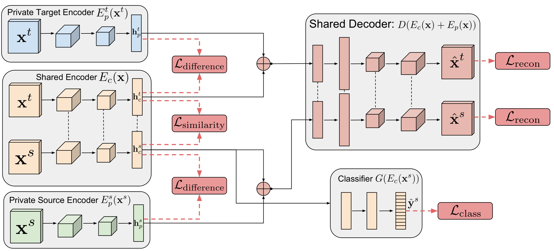
More specifically, let ${\boldsymbol{\mathbf{X}}}_S = {({\boldsymbol{\mathbf{x}}}_i^s, {\boldsymbol{\mathbf{y}}}i^s)}{i=0}^{N_s}$ represent a labeled dataset of $N_s$ samples from the source domain where ${\boldsymbol{\mathbf{x}}}_i^s \sim {\cal D}_S$ and let ${\boldsymbol{\mathbf{X}}}^t = {{\boldsymbol{\mathbf{x}}}i^t}{i=0}^{N_t}$ represent an unlabeled dataset of $N_t$ samples from the target domain where ${\boldsymbol{\mathbf{x}}}_i^t \sim {\cal D}_T$. Let $E_c(\boldsymbol{\mathbf{x}};\boldsymbol{\mathbf{\theta}}_c)$ be a function parameterized by $\boldsymbol{\mathbf{\theta}}_c$ which maps an image $\boldsymbol{\mathbf{x}}$ to a hidden representation $\boldsymbol{\mathbf{h}}_c$ representing features that are common or shared across domains. Let $E_p(\boldsymbol{\mathbf{x}};\boldsymbol{\mathbf{\theta}}_p)$ be an analogous function which maps an image $\boldsymbol{\mathbf{x}}$ to a hidden representation $\boldsymbol{\mathbf{h}}_p$ representing features that are private to each domain. Let $D(\boldsymbol{\mathbf{h}};\boldsymbol{\mathbf{\theta}}_d)$ be a decoding function mapping a hidden representation $\boldsymbol{\mathbf{h}}$ to an image reconstruction $\hat{\boldsymbol{\mathbf{x}}}$. Finally, $G(\boldsymbol{\mathbf{h}}; \boldsymbol{\mathbf{\theta}}_g)$ represents a task-specific function, parameterized by $\boldsymbol{\mathbf{\theta}}_g$ that maps from hidden representations $\boldsymbol{\mathbf{h}}$ to the task-specific predictions $\hat{\boldsymbol{\mathbf{y}}}$. The resulting Domain Separation Network (DSN) model is depicted in Figure 1.
3.1 Learning
Inference in a DSN model is given by $\hat{\boldsymbol{\mathbf{x}}} = D(E_c(\boldsymbol{\mathbf{x}}) + E_p(\boldsymbol{\mathbf{x}}))$ and $\hat{\boldsymbol{\mathbf{y}}} = G(E_c(\boldsymbol{\mathbf{x}}))$ where $\hat{\boldsymbol{\mathbf{x}}}$ is the reconstruction of the input $\boldsymbol{\mathbf{x}}$ and $\hat{\boldsymbol{\mathbf{y}}}$ is the task-specific prediction. The goal of training is to minimize the following loss with respect to parameters ${\boldsymbol{\mathbf{\Theta}} = {\boldsymbol{\mathbf{\theta}}_c, \boldsymbol{\mathbf{\theta}}_p, \boldsymbol{\mathbf{\theta}}_d, \boldsymbol{\mathbf{\theta}}_g}}$:
$ \begin{aligned} \mathcal{L} ;=; & \mathcal {L}\mathrm{task} + \alpha ;\mathcal {L}\mathrm{recon};+ ; \beta; \mathcal {L}\mathrm{difference}; +; \gamma; \mathcal {L}\mathrm{similarity} \end{aligned} $
where $\alpha, \beta, \gamma$ are weights that control the interaction of the loss terms. The classification loss $\mathcal{L}_\mathrm{task}$ trains the model to predict the output labels we are ultimately interested in. Because we assume the target domain is unlabeled, the loss is applied only to the source domain. We want to minimize the negative log–likelihood of the ground truth class for each source domain sample:
$ \mathcal {L}\mathrm{task} = -\sum{i=0}^{N_s}\boldsymbol{\mathbf{y}}_i^s\cdot \log \hat{\boldsymbol{\mathbf{y}}}_i^s, $
where $\boldsymbol{\mathbf{y}}_i^s$ is the one–hot encoding of the class label for source input $i$ and $\hat{\boldsymbol{\mathbf{y}}}_i^s$ are the softmax predictions of the model: $\hat{\boldsymbol{\mathbf{y}}}_i^s = G(E_c(\boldsymbol{\mathbf{x}}i^s))$. We use a scale–invariant mean squared error term [19] for the reconstruction loss $\mathcal{L}\mathrm{recon}$ which is applied to both domains:
$ \begin{aligned} \mathcal{L}\mathrm{recon} &= \sum{i=1}^{N_s} \mathcal{L}_\mathrm{si_mse}({\boldsymbol{\mathbf{x}}}_i^s, \hat{{\boldsymbol{\mathbf{x}}}}_i^s)
- \sum_{i=1}^{N_t} \mathcal{L}_\mathrm{si_mse}({\boldsymbol{\mathbf{x}}}_i^t, \hat{{\boldsymbol{\mathbf{x}}}}i^t) \ \mathcal{L}\mathrm{si_mse}({\boldsymbol{\mathbf{x}}}, \hat{{\boldsymbol{\mathbf{x}}}}) &= \frac{1}{k} |{\boldsymbol{\mathbf{x}}}-\hat{{\boldsymbol{\mathbf{x}}}}|_2^2 - \frac{1}{k^2}([{\boldsymbol{\mathbf{x}}}-\hat{{\boldsymbol{\mathbf{x}}}}] \cdot {\boldsymbol{\mathbf{1}}}_k)^2, \end{aligned} $
where $k$ is the number of pixels in input $x$, $\boldsymbol{\mathbf{1}}_k$ is a vector of ones of length $k$; and $|\cdot|_2^2$ is the squared $L_2$-norm. While a mean squared error loss is traditionally used for reconstruction tasks, it penalizes predictions that are correct up to a scaling term. Conversely, the scale-invariant mean squared error penalizes differences between pairs of pixels. This allows the model to learn to reproduce the overall shape of the objects being modeled without expending modeling power on the absolute color or intensity of the inputs. We validated that this reconstruction loss was indeed the correct choice experimentally in Section 4.3 by training a version of our best DSN model with the traditional mean squared error loss instead of the one in Equation 2.
The difference loss is also applied to both domains and encourages the shared and private encoders to encode different aspects of the inputs. We define the loss via a soft subspace orthogonality constraint between the private and shared representation of each domain. Let $\boldsymbol{\mathbf{H}}_c^s$ and $\boldsymbol{\mathbf{H}}_c^t$ be matrices whose rows are the hidden shared representations $\boldsymbol{\mathbf{h}}_c^s = E_c({\boldsymbol{\mathbf{x}}}^s)$ and $\boldsymbol{\mathbf{h}}_c^t = E_c({\boldsymbol{\mathbf{x}}}^t)$ from samples of source and target data respectively. Similarly, let $\boldsymbol{\mathbf{H}}_p^s$ and $\boldsymbol{\mathbf{H}}_p^t$ be matrices whose rows are the private representation $\boldsymbol{\mathbf{h}}_p^s=E_p^s({\boldsymbol{\mathbf{x}}}^s)$ and $\boldsymbol{\mathbf{h}}_p^t=E_p^t({\boldsymbol{\mathbf{x}}}^t)$ from samples of source and target data respectively. The difference loss encourages orthogonality between the shared and the private representations of each domain:
$ L_\mathrm{difference};=; \left|{\boldsymbol{\mathbf{H}}_c^s}^\top \boldsymbol{\mathbf{H}}_p^s\right|_F^2 ; + ; \left|{\boldsymbol{\mathbf{H}}_c^t}^\top \boldsymbol{\mathbf{H}}_p^t\right|_F^2, $
where $|\cdot|_F^2$ is the squared Frobenius norm. Finally, the similarity loss encourages the hidden representations ${\boldsymbol{\mathbf{h}}}_c^s$ and ${\boldsymbol{\mathbf{h}}}_c^t$ from the shared encoder to be as similar as possible irrespective of the domain. We experimented with two similarity losses, which we discuss in detail.
3.2 Similarity Losses
The domain adversarial similarity loss [11, 4] is used to train a model to produce representations such that a classifier cannot reliably predict the domain of the encoded representation. Maximizing such "confusion" is achieved via a Gradient Reversal Layer (GRL) and a domain classifier trained to predict the domain producing the hidden representation. The GRL has the same output as the identity function, but reverses the gradient direction. Formally, for some function $f(\boldsymbol{\mathbf{u}})$, the GRL is defined as $Q\left(f(\boldsymbol{\mathbf{u}})\right) = f(\boldsymbol{\mathbf{u}})$ with a gradient ${\frac{d}{d\boldsymbol{\mathbf{u}}}Q(f(\boldsymbol{\mathbf{u}}))=-\frac{d}{d\boldsymbol{\mathbf{u}}}f(\boldsymbol{\mathbf{u}})}$. The domain classifier $Z(Q(\boldsymbol{\mathbf{h}}_c); \boldsymbol{\mathbf{\theta}}_z) \rightarrow \hat{d}$ parameterized by $\boldsymbol{\mathbf{\theta}}_z$ maps a shared representation vector $\boldsymbol{\mathbf{h}}_c=E_c(\boldsymbol{\mathbf{x}} ; \boldsymbol{\mathbf{\theta}}_c)$ to a prediction of the label $\hat{d} \in {0,1}$ of the input sample ${\boldsymbol{\mathbf{x}}}$. Learning with a GRL is adversarial in that $\boldsymbol{\mathbf{\theta}}_z$ is optimized to increase $Z
#39;s ability to discriminate between encodings of images from the source or target domains, while the reversal of the gradient results in the model parameters $\boldsymbol{\mathbf{\theta}}_c$ learning representations from which domain classification accuracy is reduced. Essentially, we maximize the binomial cross–entropy for the domain prediction task with respect to $\boldsymbol{\mathbf{\theta}}_z$, while minimizing it with respect to $\boldsymbol{\mathbf{\theta}}_c$:$ \mathcal {L}\mathrm{similarity}^\mathrm{DANN} = ;\sum{i=0}^{N_s+N_t} \left{d_i \log \hat{d}_i ;+; (1-d_i) \log(1- \hat{d}_i)\right}. $
where $d_i \in {0,1}$ is the ground truth domain label for sample $i$.
The Maximum Mean Discrepancy (MMD) loss [13] is a kernel-based distance function between pairs of samples. We use a biased statistic for the squared population MMD between shared encodings of the source samples $\boldsymbol{\mathbf{h}}_c^s$ and the shared encodings of the target samples $\boldsymbol{\mathbf{h}}_c^t$:
$ \mathcal {L}\mathrm{similarity}^\mathrm{MMD};=; \displaystyle \frac{1}{(N^s)^2} \sum{i,j=0}^{N^s}\kappa(\boldsymbol{\mathbf{h}}{ci}^s, \boldsymbol{\mathbf{h}}{cj}^s)-\frac{2}{N^sN^t}\sum_{i,j=0}^{N^s,N^t}\kappa(\boldsymbol{\mathbf{h}}{ci}^s, \boldsymbol{\mathbf{h}}{cj}^t) + \frac{1}{(N^t)^2}\sum_{i,j=0}^{N^t}\kappa(\boldsymbol{\mathbf{h}}{ci}^t,\boldsymbol{\mathbf{h}}{cj}^t), $
where $\kappa(\cdot,\cdot)$ is a PSD kernel function. In our experiments we used a linear combination of multiple RBF kernels: $\kappa(x_i, x_j) = \sum_n \eta_n \exp {-\frac{1}{2\sigma_n}|\boldsymbol{\mathbf{x}}_i - \boldsymbol{\mathbf{x}}_j|^2}$, where $\sigma_n$ is the standard deviation and $\eta_n$ is the weight for our $n^{th}$ RBF kernel. Any additional kernels we include in the multi–RBF kernel are additive and guarantee that their linear combination remains characteristic. Therefore, having a large range of kernels is beneficial since the distributions of the shared features change during learning, and different components of the multi–RBF kernel might be responsible at different times for making sure we reject a false null hypothesis, i.e. that the loss is sufficiently high when the distributions are not similar [6]. The advantage of using an RBF kernel with the MMD distance is that the Taylor expansion of the Gaussian function allows us to match all the moments of the two populations. The caveat is that it requires finding optimal kernel bandwidths $\sigma_n$.
4. Evaluation
Section Summary: The evaluation examines how well models trained on clean synthetic images can adapt to noisy real-world data for object classification, using scenarios that shift between datasets such as MNIST to MNIST-M, SVHN to MNIST, and synthetic to real traffic signs or objects. The authors compare their approach with two similarity losses against prior methods like CORAL, DANN, and MMD regularization, showing stronger results than the baselines while also testing on a held-out validation set of labeled target examples to tune hyperparameters. They note that fully unsupervised validation remains difficult and that their method reaches the highest accuracy across most of the tested shifts.
We are motivated by the problem of learning models on a clean, synthetic dataset and testing on noisy, real–world dataset. To this end, we evaluate on object classification datasets used in previous work[^1] including MNIST and MNIST-M [4], the German Traffic Signs Recognition Benchmark (GTSRB) [20], and the Streetview House Numbers (SVHN) [21]. We also evaluate on the cropped LINEMOD dataset, a standard for object instance recognition and 3D pose estimation [22, 23], for which we have synthetic and real data[^2]. We tested the following unsupervised domain adaptation scenarios: (a) from MNIST to MNIST-M; (b) from SVHN to MNIST; (c) from synthetic traffic signs to real ones with GTSRB; (d) from synthetic LINEMOD object instances rendered on a black background to the same object instances in the real world.
[^1]: The most commonly used dataset for visual domain adaptation in the context of object classification is Office [24]. However, this dataset exhibits significant variations in both low-level and high-level parameter distributions. Low-level variations are due to the different cameras and background textures in the images (e.g. Amazon versus DSLR). However, there are significant high-level variations due to object identity: e.g. the motorcycle class contains non-motorcycle objects; the backpack class contains a laptop; some domains contain the object in only one pose. Other commonly used datasets such as Caltech-256 suffer from similar problems. We therefore exclude these datasets from our evaluation. For more information, see our Supplementary Material.
[^2]: https://cvarlab.icg.tugraz.at/projects/3 $d_o$ bject_detection/
We evaluate the efficacy of our method with each of the two similarity losses outlined in Section 3.2 by comparing against the prevailing visual domain adaptation techniques for neural networks: Correlation Alignment (CORAL) [3], Domain–Adversarial Neural Networks (DANN) [11, 4], and MMD regularization [8, 6]. For each scenario we provide two additional baselines: the performance on the target domain of the respective model with no domain adaptation and trained (a) on the source domain ("Source–only" in Table 4) and (b) on the target domain ("Target–only"), as an empirical lower and upper bound respectively.
We have not found a universally applicable way to optimize hyperparameters for unsupervised domain adaptation. Previous work [4] suggests the use of reverse validation. We implemented this (see Supplementary Material for details) but found that that the reverse validation accuracy did not always align well with test accuracy. Ideally we would like to avoid using labels from the target domain, as it can be argued that if ones does have target domain labels, they should be used during training. However, there are applications where a labeled target domain set cannot be used for training. An example is the labeling of a dataset with the use of AprilTags [25], 2D barcodes that can be used to label the pose of an object, provided that a camera is calibrated and the physical dimensions of the barcode are known. These images should not be used when learning features from pixels, because the model might be able to decipher the tags. However, they can be part of a test set that is not available during training, and an equivalent dataset without the tags could be used for unsupervised domain adaptation. We thus chose to use a small set of labeled target domain data as a validation set for the hyperparameters of all the methods we compare. All methods were evaluated using the same protocol, so comparison numbers are fair and meaningful. The performance on this validation set can serve as an upper bound of a satisfactory validation metric for unsupervised domain adaptation, which to our knowledge is still an open research question, and out of the scope of this work.
: Table 1: Mean classification accuracy (%) for the unsupervised domain adaptation scenarios we evaluated all the methods on. We have replicated the experiments from Ganin et al. [4] and in parentheses we show the results reported in their paper. The "Source–only" and "Target–only" rows are the results on the target domain when using no domain adaptation and training only on the source or the target domain respectively. The results that perform best in each domain adaptation task are in bold font.
| Model | MNIST to | Synth Digits to | SVHN to | Synth Signs to |
|---|---|---|---|---|
| MNIST-M | SVHN | MNIST | GTSRB | |
| Source-only | 56.6 (52.2) | 86.7 (86.7) | 59.2 (54.9) | 85.1 (79.0) |
| CORAL [3] | 57.7 | 85.2 | 63.1 | 86.9 |
| MMD [8, 6] | 76.9 | 88.0 | 71.1 | 91.1 |
| DANN [4] | 77.4 (76.6) | 90.3 (91.0) | 70.7 (73.8) | 92.9 (88.6) |
| DSN w/ MMD (ours) | 80.5 | 88.5 | 72.2 | 92.6 |
| DSN w/ DANN (ours) | 83.2 | 91.2 | 82.7 | 93.1 |
| Target-only | 98.7 | 92.4 | 99.5 | 99.8 |
4.1 Datasets and Adaptation Scenarios
MNIST to MNIST-M. In this domain adaptation scenario we use the popular MNIST [26] dataset of handwritten digits as the source domain, and MNIST-M, a variation of MNIST proposed for unsupervised domain adaptation by [4]. MNIST-M was created by using each MNIST digit as a binary mask and inverting with it the colors of a background image. The background images are random crops uniformly sampled from the Berkeley Segmentation Data Set (BSDS500) [27]. In all our experiments, following the experimental protocol by [4]. Out of the $59,001$ MNIST-M training examples, we used the labels for $1,000$ of them to find optimal hyperparameters for our models. This scenario, like all three digit adaptation scenarios, has 10 class labels.
Synthetic Digits to SVHN. In this scenario we aim to learn a classifier for the Street-View House Number data set (SVHN) [21], our target domain, from a dataset of purely synthesized digits, our source domain. The synthetic digits [4] dataset was created by rasterizing bitmap fonts in a sequence (one, two, and three digits) with the ground truth label being the digit in the center of the image, just like in SVHN. The source domain samples are further augmented by variations in scale, translation, background colors, stroke colors, and Gaussian blurring. We use $479,400$ Synthetic Digits for our source domain training set, $73,257$ unlabeled SVHN samples for domain adaptation, and $26,032$ SVHN samples for testing. Similarly to above, we used the labels of $1,000$ SVHN training examples to find optimal hyperparameters for our models.
SVHN to MNIST. Although the SVHN dataset contains significant variations (in scale, background clutter, blurring, embossing, slanting, contrast, rotation, sequences to name a few) there is not a lot of variation in the actual digits shapes. This makes it quite distinct from a dataset of handwritten digits, like MNIST, where there are a lot of elastic distortions in the shapes, variations in thickness, and noise on the digits themselves. Since the ground truth digits in both datasets are centered, this is a well–posed and rather difficult domain adaptation scenario. As above, we used the labels of $1,000$ MNIST training examples for validation.
Synthetic Signs to GTSRB. We also perform an experiment using a dataset of synthetic traffic signs from [28] to real world dataset of traffic signs (GTSRB) [20]. While the three digit adaptation scenarios have 10 class labels, this scenario has 43 different traffic signs. The synthetic signs were obtained by taking relevant pictograms and adding various types of variations, including random backgrounds, brightness, saturation, 3D rotations, Gaussian and motion blur. We use $90,000$ synthetic signs for training, $1,280$ random GTSRB real–world signs for domain adaptation and validation, and the remaining $37,929$ GTSRB real signs as the test set.
Synthetic Objects to LineMod. The LineMod dataset [23] consists of CAD models of objects in a cluttered environment and a high variance of 3D poses for each object. We use the 11 non–symmetric objects from the cropped version of the dataset, where the images are cropped with the object in the center, for the task of object instance recognition and 3D pose estimation. We train our models on $16,962$ images for these objects rendered on a black background without additional noise. We use a target domain training set of $10,673$ real–world images for domain adaptation and validation, and a target domain test set of $2,655$ for testing. For this scenario our task is both classification and pose estimation; our task loss is therefore $\mathcal{L}\mathrm{task}=\sum{i=0}^{N_s}{-\boldsymbol{\mathbf{y}}_i^s\cdot \log \hat{\boldsymbol{\mathbf{y}}}_i^s+\xi \log(1-|\boldsymbol{\mathbf{q}}^s\cdot \hat{\boldsymbol{\mathbf{q}}}^s|)}$, where $\boldsymbol{\mathbf{q}}^s$ is the positive unit quaternion vector representing the ground truth 3D pose, and $\hat{\boldsymbol{\mathbf{q}}}^s$ is the equivalent prediction. The first term is the classification loss, similar to the rest of the experiments, the second term is the log of a 3D rotation metric for quaternions [29], and $\xi$ is the weight for the pose loss. Quaternions are a convenient angle–axis representation for 3D rotations. In Table 2 we report the mean angle the object would need to be rotated (on a fixed 3D axis) to move from the predicted pose to the ground truth [22].
\begin{tabular}{@|l|c|c|@}
\hline
\multicolumn{1}{|c|}{\textbf{Method}} & \multicolumn{1}{c|}{\textbf{Classification Accuracy}} & \multicolumn{1}{c|}{\textbf{Mean Angle Error}} \\ \hline \hline
Source-only & 47.33\% & $89.2^{\circ}$\\\hline \hline
MMD & 72.35\% & $70.62^{\circ}$ \\ \hline
DANN & 99.90\% &$56.58^{\circ}$ \\ \hline\hline
DSN w/ MMD (ours) & 99.72\% &$66.49^{\circ}$\\ \hline
DSN w/ DANN (ours) & \textbf{100.00}\% & $\textbf{53.27}^{\circ}$\\ \hline\hline
Target-only & 100.00\% &$6.47^{\circ}$ \\ \hline
\end{tabular}
4.2 Implementation Details
All the models were implemented using TensorFlow[^3] [30] and were trained with Stochastic Gradient Descent plus momentum [31]. Our initial learning rate was multiplied by $0.9$ every $20,000$ steps (mini-batches). We used batches of 32 samples from each domain for a total of 64 and the input images were mean-centered and rescaled to $[-1, 1]$. In order to avoid distractions for the main classification task during the early stages of the training procedure, we activate any additional domain adaptation loss after $10,000$ steps of training. For all our experiments our CNN topologies are based on the ones used in [4], to be comparable to previous work in unsupervised domain adaptation. The exact architectures for all models are shown in our Supplementary Material.
[^3]: Our code will be open–sourced under https://github.com/tensorflow/models/ before the NIPS 2016 meeting.
In our framework, CORAL [3] would be equivalent to fixing our shared representation matrices $\boldsymbol{\mathbf{H}}_c^s$ and $\boldsymbol{\mathbf{H}}_c^t$, normalizing them and then minimizing $| \boldsymbol{\mathbf{A}}{\boldsymbol{\mathbf{H}}_c^s}^\top {\boldsymbol{\mathbf{H}}_c^s}\boldsymbol{\mathbf{A}}^\top - {\boldsymbol{\mathbf{H}}_c^t}^\top {\boldsymbol{\mathbf{H}}c^t} |F^2$ with respect to a weight matrix $\boldsymbol{\mathbf{A}}$ that aligns the two correlation matrices. For the CORAL experiments, we follow the suggestions of [3], and extract features for both source and target domains from the penultimate layer of each network. Once the correlation matrices for each domain are aligned, we evaluate on the target test data the performance of a linear support vector machine (SVM) classifier trained on the source training data. The SVM penalty parameter was optimized based on the target domain validation set for each of our domain adaptation scenarios. For MMD regularization, we used a linear combination of 19 RBF kernels[^4]. We applied MMD on fc3 on all our model architectures and minimized $\mathcal {L}=\mathcal {L}\mathrm{class}+\gamma; \mathcal {L}\mathrm{similarity}^\mathrm{MMD}$ with respect to $\boldsymbol{\mathbf{\theta}}c,\boldsymbol{\mathbf{\theta}}g$. Preliminary experiments with having MMD applied on more than one layers did not show any performance improvement for our experiments and architectures. For DANN regularization, we applied the GRL and the domain classifier as prescribed in [4] for each scenario. We optimized $\mathcal {L}=\mathcal {L}\mathrm{class}+\gamma; \mathcal {L}\mathrm{similarity}^\mathrm{DANN}$ by minimizing it with respect to $\boldsymbol{\mathbf{\theta}}_c,\boldsymbol{\mathbf{\theta}}_g$ and maximizing it with respect to the domain classifier parameters $\boldsymbol{\mathbf{\theta}}_z$.
[^4]: The Supplementary Material has details on all the parameters.
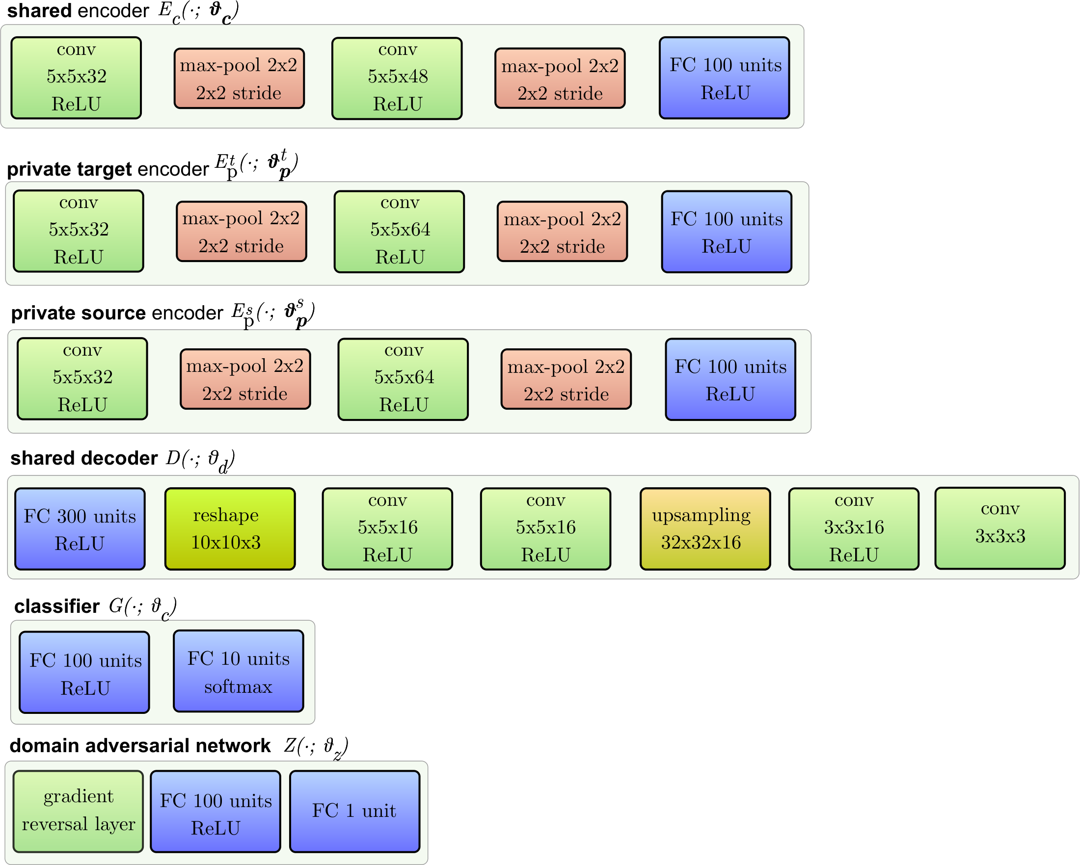
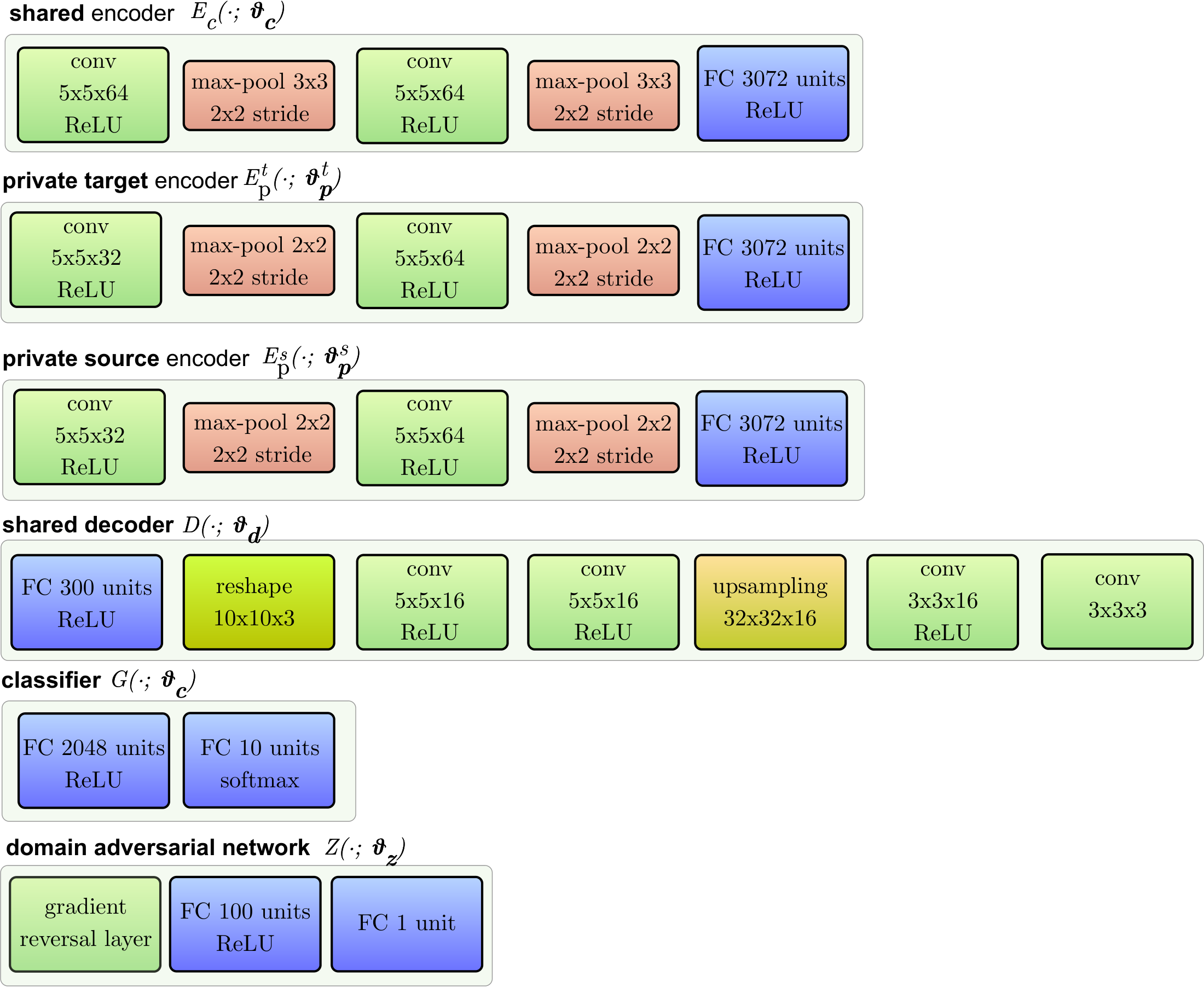
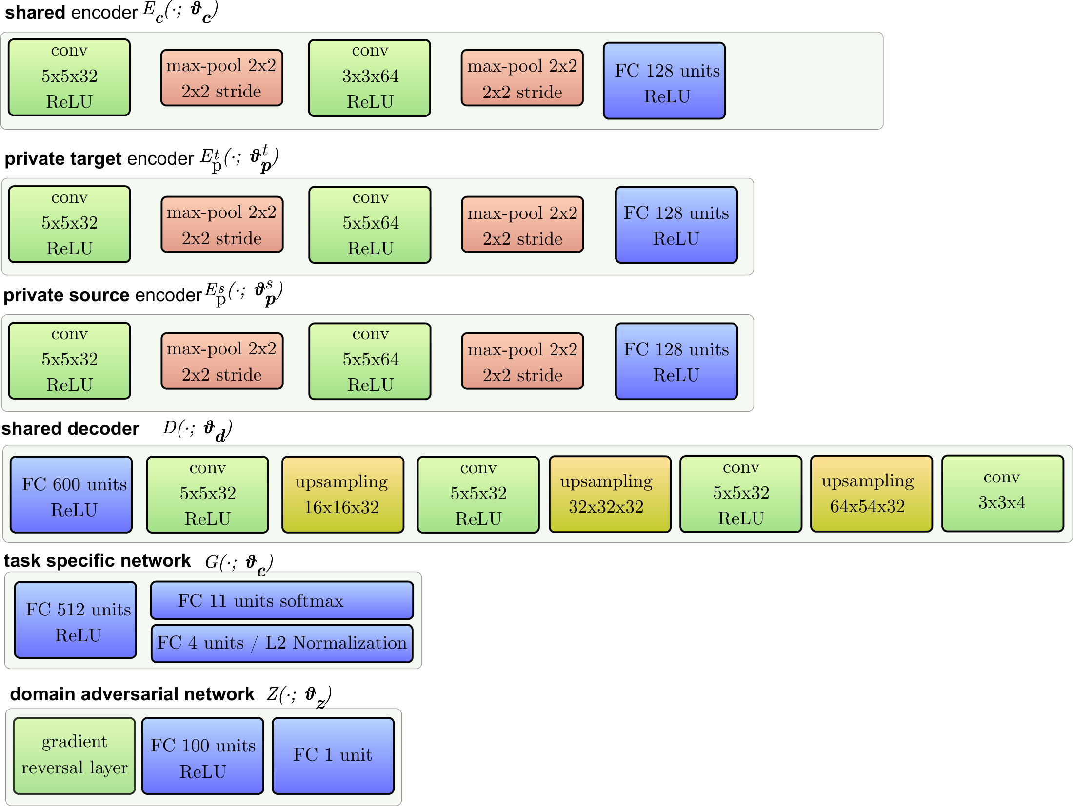
For our Domain Separation Network experiments, our similarity losses are always applied at the first fully connected layer of each network after a number of convolutional and max pooling layers. For each private space encoder network we use a simple convolutional and max pooling structure followed by a fully-connected layer with a number of nodes equal to the number of nodes at the final layer $\boldsymbol{\mathbf{h}}_c$ of the equivalent shared encoder $E_c$. The output of the shared and private encoders gets added before being fed to the shared decoder $D$. For the latter we use a deconvolutional architecture [32] which consists of a fully connected layer with 300 nodes, a resizing layer to $10\times10\times3$, two $3\times3\times16$ convolutional layers, one upsampling layer to $32\times32\times16$, another $3\times3\times16$ convolutional layer, followed by the reconstruction output.
4.3 Discussion
The DSN with DANN model outperforms all the other methods we experimented with for all our unsupervised domain adaptation scenarios (see Table 4 and Table 2). Our unsupervised domain separation networks are able to improve both upon MMD regularization and DANN. Using DANN as a similarity loss Equation (4) worked better than using MMD Equation (5) as a similarity loss, which is consistent with results obtained for domain adaptation using MMD regularization and DANN alone.
In order to examine the effect of the soft orthogonality constraints ($\mathcal{L}\mathrm{difference}$), we took our best model, our DSN model with the DANN loss, and removed these constraints by setting the $\beta$ coefficient to $0$. Without them, the model performed consistently worse in all scenarios. We also validated our choice of our scale–invariant mean squared error reconstruction loss as opposed to the more popular mean squared error loss by running our best model with $\mathcal{L}\mathrm{recon}^{{L2}}=\frac{1}{k}||{x}-\hat{{x}}||_2^2$. With this variation we also get worse classification results consistently, as shown in experiments from Table 3.
::: {caption="Table 3: Effect of our difference and reconstruction losses on our best model. The first row is replicated from Table 4. In the second row, we remove the soft orthogonality constraint. In the third row, we replace the scale–invariant MSE with regular MSE."}

:::
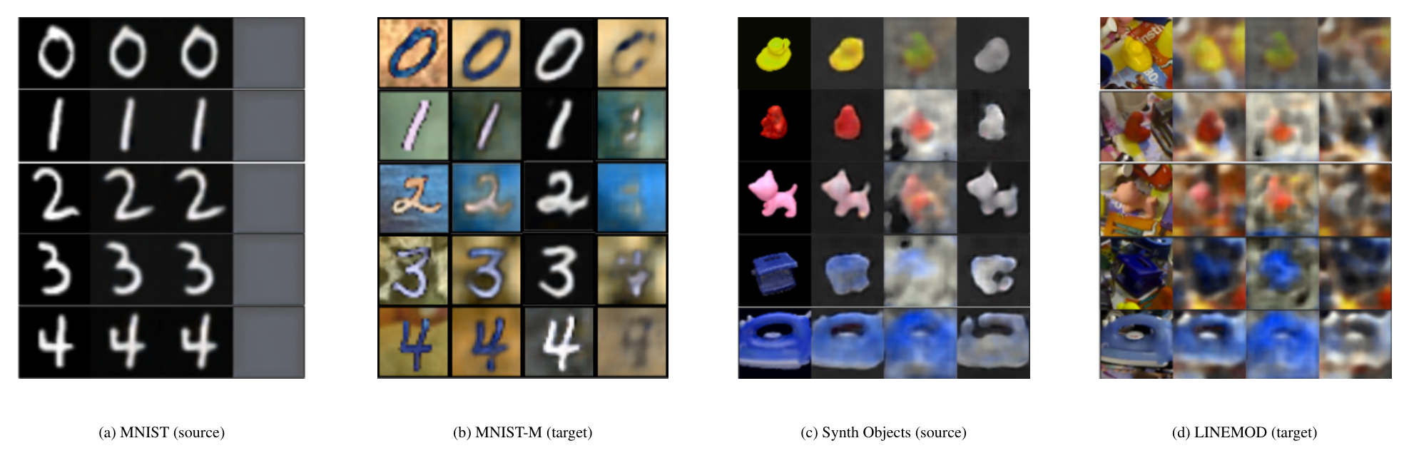
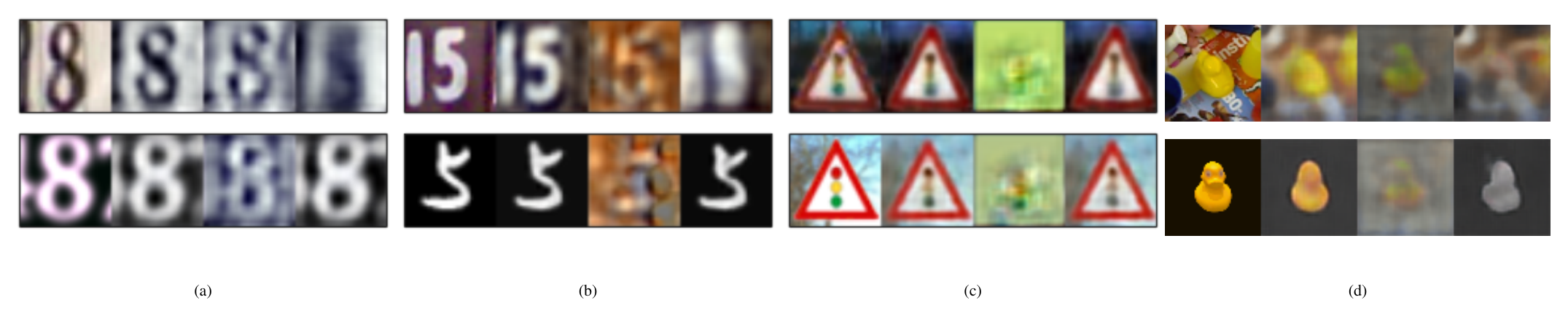
The shared and private representations of each domain are combined for the reconstruction of samples. Individually decoding the shared and private representations gives us reconstructions that serve as useful depictions of our domain adaptation process. In Figure 2 we use the "MNIST to MNIST-M" and the "Synth. Objects to LINEMOD" scenarios for such visualizations. In the former scenario, the model clearly separates the foreground from the background and produces a shared space that is very similar to the source domain. This is expected since the target is a transformation of the source. In the latter scenario, the model is able to produce visualizations of the shared representation that look very similar between source and target domains, which are useful for classification and pose estimation, as shown in Table 2.
5. Conclusion
Section Summary: This work introduces a deep learning model that advances unsupervised domain adaptation by separating features unique to each domain from those shared across source and target domains. It aligns the shared features using existing adaptation techniques while applying constraints to keep private and shared features distinct. The approach leads to better performance than prior methods in several scenarios that transfer knowledge from synthetic to real data.
We present in this work a deep learning model that improves upon existing unsupervised domain adaptation techniques. The model does so by explicitly separating representations private to each domain and shared between source and target domains. By using existing domain adaptation techniques to make the shared representations similar, and soft subspace orthogonality constraints to make private and shared representations dissimilar, our method outperforms all existing unsupervised domain adaptation methods in a number of adaptation scenarios that focus on the synthetic–to–real paradigm.
Acknowledgments
We would like to thank Samy Bengio, Kevin Murphy, and Vincent Vanhoucke for valuable comments on this work. We would also like to thank Yaroslav Ganin and Paul Wohlhart for providing some of the datasets we used.
Supplementary Material
Appendix
Section Summary: The appendix first presents Correlation Regularization, a new domain-adaptation technique that aligns second-order statistics between source and target feature representations; experiments show it outperforms the earlier CORAL method on several digit and sign datasets, and combining it with domain-separation networks yields further gains. It then criticizes the widely used Office object-classification benchmark for problems such as label pollution, inconsistent object poses, and background variations that complicate fair evaluation. Finally, the section supplies qualitative visualizations of shared and private feature reconstructions across multiple domain pairs together with the network architectures and hyper-parameters needed to reproduce the reported results.
A. Correlation Regularization
Correlation Alignment (CORAL) [3] aims to find a mapping from the representations of the source domain to the representations of the target domain by matching only the second–order statistics. In our framework, this would be equivalent to fixing our common representation matrices $\boldsymbol{\mathbf{H}}_c^s$ and $\boldsymbol{\mathbf{H}}c^t$ after normalizing them and then finding a weight matrix $\hat{\boldsymbol{\mathbf{A}}} = \displaystyle {\operatorname*{argmin}{\boldsymbol{\mathbf{A}}}}\left| \boldsymbol{\mathbf{A}}{\boldsymbol{\mathbf{H}}_c^s}^\top {\boldsymbol{\mathbf{H}}_c^s}\boldsymbol{\mathbf{A}}^\top - {\boldsymbol{\mathbf{H}}_c^t}^\top {\boldsymbol{\mathbf{H}}_c^t} \right|_F^2$ that aligns the two correlation matrices. Although this has the advantage that the optimization is convex and can be solved in closed form, all convolutional features remain fixed during the process, which might not be optimal for the task at hand. Also, because of this we are not able to use it as a similarity loss for our DSNs. Motivated by this shortcoming, we propose here a new domain adaptation method, Correlation Regularization (CorReg). We show in Table 4 that our new domain adaptation method, which is theoretically as powerful as an MMD loss with a second–order polynomial kernel, outperforms CORAL in all our datasets. Adapting a feature hierarchy to be domain–invariant is more powerful than learning a mapping from the representations of one domain to those of another. Moreover, we use it as yet another similarity loss for our Domain Separation Networks:
$ \mathcal{L}_\mathrm{similarity}^\mathrm{CorReg} = \left| {\boldsymbol{\mathbf{H}}_c^s}^\top {\boldsymbol{\mathbf{H}}_c^s} - {\boldsymbol{\mathbf{H}}_c^t}^\top {\boldsymbol{\mathbf{H}}_c^t} \right|_F^2 $
Our DNS with CorReg performs better than both CORAL and CorReg, which is consistent with the rest of our results.
: Table 1: Our main results from the paper with two additional lines for CorReg and DSN with CorReg.
| Model | MNIST to | Synth Digits to | SVHN to | Synth Signs to |
|---|---|---|---|---|
| MNIST-M | SVHN | MNIST | GTSRB | |
| Source-only | 56.6 (52.2) | 86.7 (86.7) | 59.2 (54.9) | 85.1 (79.0) |
| CORAL [3] | 57.7 | 85.2 | 63.1 | 86.9 |
| CorReg (Ours) | 62.06 | 87.33 | 69.20 | 90.75 |
| MMD [8, 6] | 76.9 | 88.0 | 71.1 | 91.1 |
| DANN [4] | 77.4 (76.6) | 90.3 (91.0) | 70.7 (73.8) | 92.9 (88.6) |
| DSN w/ MMD (ours) | 80.5 | 88.5 | 72.2 | 92.6 |
| DSN w/ DANN (ours) | 83.2 | 91.2 | 82.7 | 93.1 |
| Target-only | 98.7 | 92.4 | 99.5 | 99.8 |
B. Office Dataset Criticism
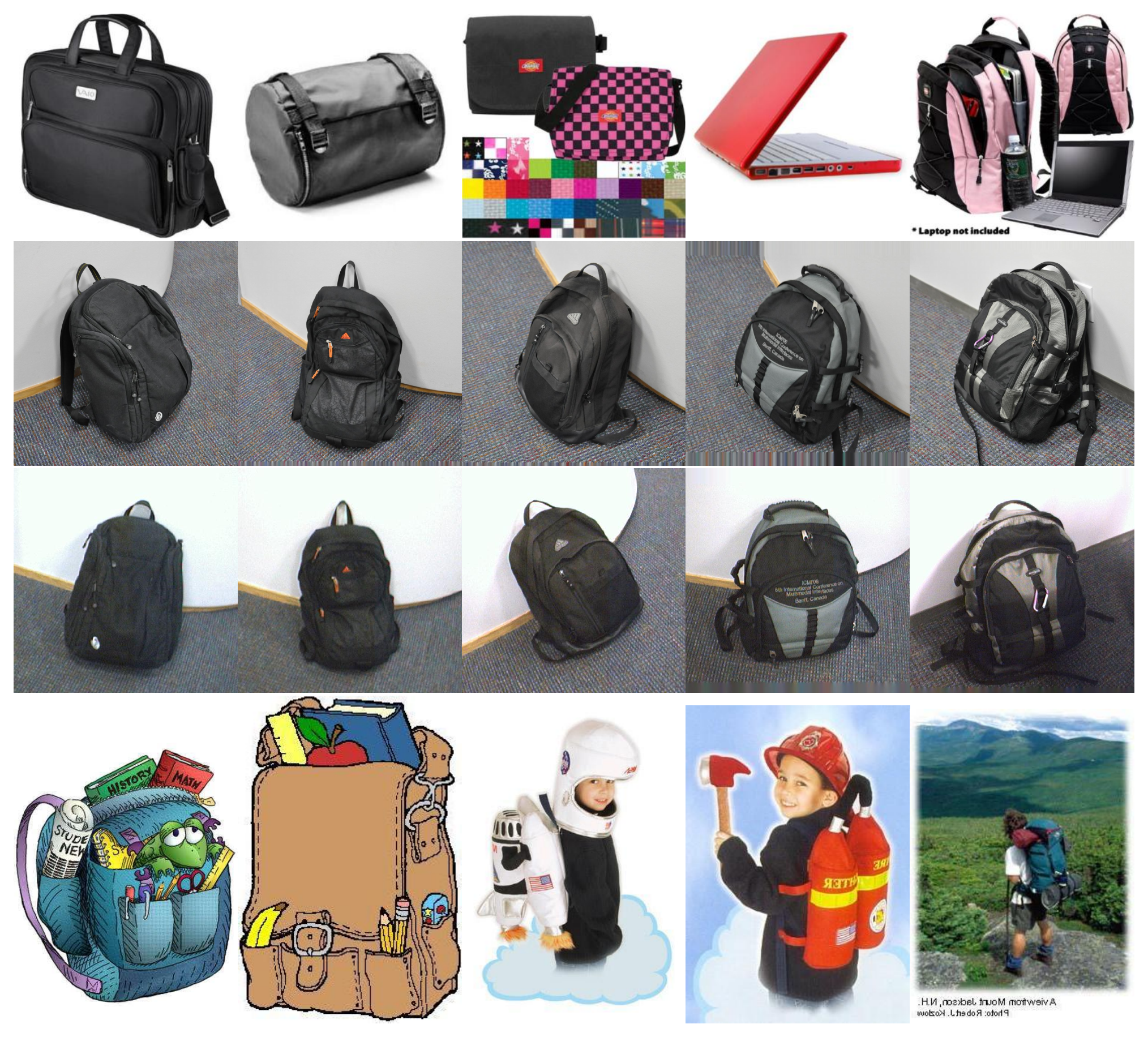
The most commonly used dataset for visual domain adaptation in the context of object classification is Office [24], sometimes combined with the Caltech–256 dataset [33] as an additional domain. However, these datasets exhibit significant variations in both low-level and high-level parameter distributions. Low-level variations are due to the different cameras and background textures in the images (e.g. Amazon versus DSLR), which is welcome. However, there are significant high-level variations due to elements like label pollution: e.g. the motorcycle class contains non-motorcycle objects; the backpack class contains 2 laptops; some classes contain the object in only one pose. Other commonly used datasets such as Caltech-256 suffer from similar problems. We illustrate some of these issues for the 'back_pack' class for its 92 Amazon samples, its 12 DSLR samples, its 29 Webcam samples, and its 151 Caltech samples in Figure 3. Other classes exhibit similar problems. For these reasons some works, eg [3], pretrain their models on Imagenet before performing the domain adaptation in these scenarios. This essentially involves another source domain (Imagenet) in the transfer.
C. Domain Separation
We visualize in Figure 4 reconstructions for both source and target domains of each domain adaptation scenario. Although the visualizations are not as clear as with the "MNIST to MNIST-M" scenario, where the target domain was a direct transformation of the source domain, it is interesting to note the similarities of the visualizations of the shared representations, and the exclusion of some shared information in the private domains.
D. Network Topologies and Optimal Parameters
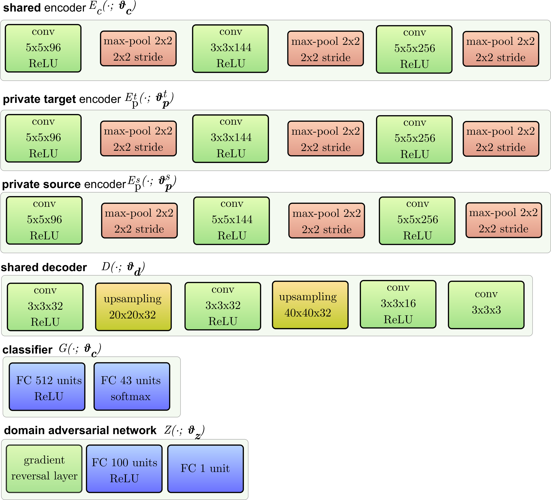
Since we used different network topologies for our domain adaptation scenarios, there was not enough space to include these in the main paper. We present the exact topologies used in Figures 5-8.
Similarly, we list here all hyperparameters that are important for total reproducibility of all our results. For CORAL, the SVM penalty parameter that was optimized based on the validation set for each of our domain adaptation scenarios: $1e^{-4}$ for "MNIST to MNIST-M", "Synth Digits to SVHN", "Synth Signs to GTSRB", and $1e^{-3}$ for "SVHN to MNIST". For MMD we use 19 RBF kernels with the following standard deviation parameters:
$ \boldsymbol{\mathbf{\sigma}} = [10^{-6}, 10^{-5}, 10^{-4}, 10^{-3}, 10^{-2}, 10^{-1}, 1, 5, 10, 15, 20, 25, 30, 35, 100, 10^{3}, 10^{4}, 10^{5}, 10^{6}] $
and equal $\eta$ weights. We use learning rate between $[0.01, 0.015]$ and $\gamma \in [0.1, 0.3]$. For DANN we use learning rate between $[0.01, 0.015]$ and $\gamma \in [0.15, 0.25]$. For DSN w/ DANN and DSN w/ MMD we use a constant initial learning rate of $0.01$ use the hyperparameters in the range of: $\alpha \in [0.01, 0.15], \beta \in [0.05, 0.075], \gamma \in [0.25, 0.3]$, whereas for DNS w/ CorReg we use $\gamma \in [20, 100]$. For the GTSRB experiment we use $\alpha \in [0.01, 0.015]$. In all cases we use an exponential decay of $0.95$ on the learning rate every $20,000$ iterations. For the LINEMOD experiments we use $\xi = 0.125$.
References
Section Summary: This section compiles a numbered list of 33 academic citations that support the paper's discussion of machine learning techniques. The references cover foundational datasets for image recognition, theoretical work on adapting models across different data sources, and practical methods involving neural networks for tasks like object detection and pose estimation. They draw primarily from recent conferences and journals in computer vision and artificial intelligence.
[1] T.-Y. Lin, M. Maire, S. Belongie, J. Hays, P. Perona, D. Ramanan, P. Dollár, and C. L. Zitnick. Microsoft coco: Common objects in context. In ECCV 2014, pages 740–755. Springer, 2014.
[2] O. Russakovsky et al. ImageNet Large Scale Visual Recognition Challenge. IJCV, 115(3):211–252, 2015.
[3] B. Sun, J. Feng, and K. Saenko. Return of frustratingly easy domain adaptation. In AAAI. 2016.
[4] Y. Ganin \etal. Domain-Adversarial Training of Neural Networks. JMLR, 17(59):1–35, 2016.
[5] E. Tzeng, J. Hoffman, T. Darrell, and K. Saenko. Simultaneous deep transfer across domains and tasks. In CVPR, pages 4068–4076, 2015.
[6] M. Long and J. Wang. Learning transferable features with deep adaptation networks. ICML, 2015.
[7] M. Salzmann et. al. Factorized orthogonal latent spaces. In AISTATS, pages 701–708, 2010.
[8] E. Tzeng, J. Hoffman, N. Zhang, K. Saenko, and T. Darrell. Deep domain confusion: Maximizing for domain invariance. Preprint arXiv:1412.3474, 2014.
[9] S. Ben-David, J. Blitzer, K. Crammer, A. Kulesza, F. Pereira, and J. W. Vaughan. A theory of learning from different domains. Machine learning, 79(1-2):151–175, 2010.
[10] Y. Mansour \etal. Domain adaptation with multiple sources. In NIPS, 2009.
[11] Y. Ganin and V. Lempitsky. Unsupervised domain adaptation by backpropagation. In ICML, pages 513–520, 2015.
[12] H. Ajakan, P. Germain, H. Larochelle, F. Laviolette, and M. Marchand. Domain-adversarial neural networks. In Preprint, http://arxiv.org/abs/1412.4446, 2014.
[13] A. Gretton, K. M. Borgwardt, M. J. Rasch, B. Schölkopf, and A. Smola. A Kernel Two-Sample Test. JMLR, pages 723–773, 2012.
[14] B. Gong, Y. Shi, F. Sha, and K. Grauman. Geodesic flow kernel for unsupervised domain adaptation. In CVPR, pages 2066–2073. IEEE, 2012.
[15] R. Caseiro, J. F. Henriques, P. Martins, and J. Batist. Beyond the shortest path: Unsupervised Domain Adaptation by Sampling Subspaces Along the Spline Flow. In CVPR, 2015.
[16] R. Gopalan, R. Li, and R. Chellappa. Domain Adaptation for Object Recognition: An Unsupervised Approach. In ICCV, 2011.
[17] Y. Jia, M. Salzmann, and T. Darrell. Factorized latent spaces with structured sparsity. In NIPS, pages 982–990, 2010.
[18] S. Virtanen, A. Klami, and S. Kaski. Bayesian CCA via group sparsity. In ICML, pages 457–464, 2011.
[19] D. Eigen, C. Puhrsch, and R. Fergus. Depth map prediction from a single image using a multi-scale deep network. In NIPS, pages 2366–2374, 2014.
[20] J. Stallkamp, M. Schlipsing, J. Salmen, and C. Igel. Man vs. computer: Benchmarking machine learning algorithms for traffic sign recognition. Neural Networks, 2012.
[21] Y. Netzer, T. Wang, A. Coates, A. Bissacco, B. Wu, and A. Y. Ng. Reading digits in natural images with unsupervised feature learning. In NIPS Workshops, 2011.
[22] S. Hinterstoisser \etal. Model based training, detection and pose estimation of texture-less 3d objects in heavily cluttered scenes. In ACCV, 2012.
[23] P. Wohlhart and V. Lepetit. Learning descriptors for object recognition and 3d pose estimation. In CVPR, pages 3109–3118, 2015.
[24] K. Saenko \etal. Adapting visual category models to new domains. In ECCV. Springer, 2010.
[25] E. Olson. Apriltag: A robust and flexible visual fiducial system. In Robotics and Automation (ICRA), 2011 IEEE International Conference on, pages 3400–3407. IEEE, 2011.
[26] Y. LeCun, L. Bottou, Y. Bengio, and P. Haffner. Gradient-based learning applied to document recognition. Proceedings of the IEEE, 86(11):2278–2324, 1998.
[27] P. Arbelaez, M. Maire, C. Fowlkes, and J. Malik. Contour detection and hierarchical image segmentation. TPAMI, 33(5):898–916, 2011.
[28] B. Moiseev, A. Konev, A. Chigorin, and A. Konushin. Evaluation of Traffic Sign Recognition Methods Trained on Synthetically Generated Data, chapter ACIVS, pages 576–583. Springer International Publishing, 2013.
[29] D. Q. Huynh. Metrics for 3d rotations: Comparison and analysis. Journal of Mathematical Imaging and Vision, 35(2):155–164, 2009.
[30] M. Abadi et al. Tensorflow: Large-scale machine learning on heterogeneous distributed systems. Preprint arXiv:1603.04467, 2016.
[31] I. Sutskever, J. Martens, G. Dahl, and G. Hinton. On the importance of initialization and momentum in deep learning. In ICML, pages 1139–1147, 2013.
[32] M. D. Zeiler, D. Krishnan, G. W. Taylor, and R. Fergus. Deconvolutional networks. In CVPR, pages 2528–2535. IEEE, 2010.
[33] G. Griffin, A. Holub, and P. Perona. Caltech-256 object category dataset. CNS-TR-2007-001, 2007.