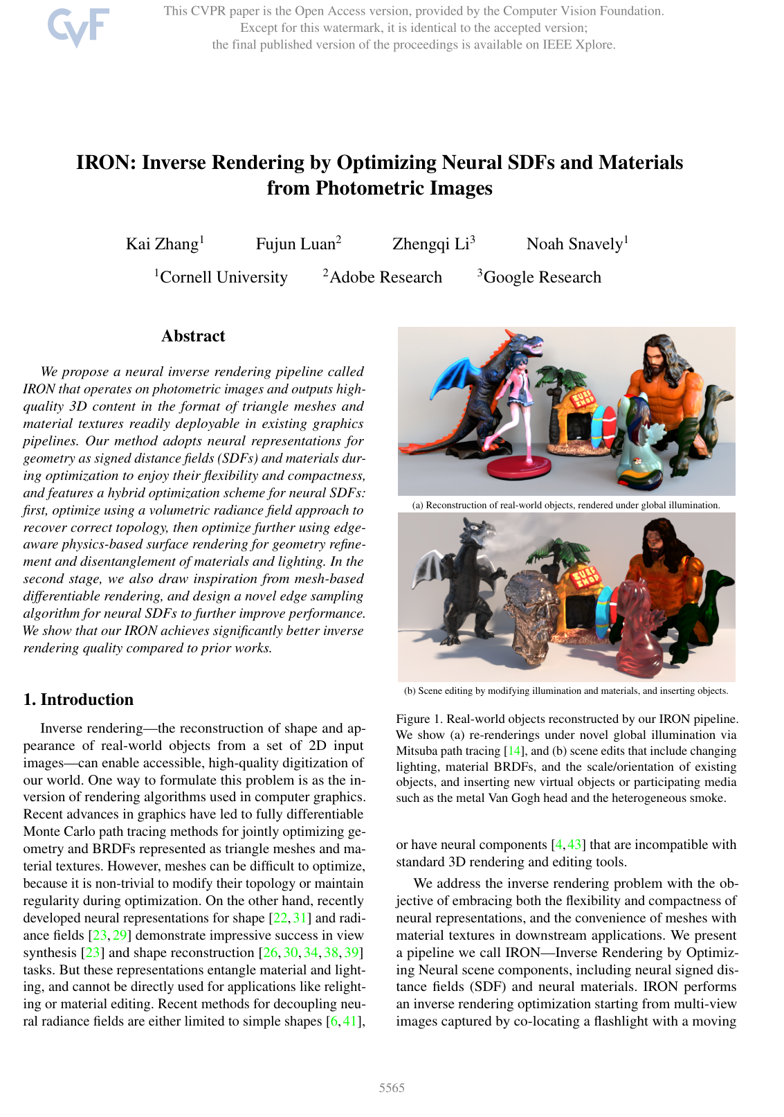
IRON: Inverse Rendering by Optimizing Neural SDFs and Materials from Photometric Images

Kai ZhangFujun LuanZhengqi LiNoah Snavely

article2022CVPR156 citations

Proposes a hybrid inverse rendering framework that couples volumetric neural signed distance fields with edge-aware physics-based surface rendering to reconstruct high-fidelity textured meshes directly compatible with standard graphics engines.

Listen

Digitizing real-world objects into high-quality 3D digital assets is a critical capability for augmented reality, virtual reality, and modern computer graphics. While traditional mesh-based methods struggle with topological changes during optimization and existing neural techniques often fuse lighting and material properties in ways incompatible with standard editing software, creating realistic, editable 3D content remains technically challenging.

The article demonstrates a novel inverse rendering pipeline called IRON that reconstructs high-fidelity 3D geometry and spatially varying material properties directly from multi-view flashlight photographs, producing assets that convert cleanly into standard triangle meshes and texture maps.

The authors evaluated the framework on synthetic datasets of nine complex objects and real-world captures of five physical subjects photographed under a co-located camera and flashlight setup. The technical approach applies a two-stage hybrid optimization: it first optimizes a neural signed distance field and diffuse albedo using volumetric radiance to establish correct global shape and topology, and then refines geometry and separates material parameters via an edge-aware physics-based surface rendering algorithm that samples subpixel depth discontinuities.

The evaluation produced several key findings. First, on synthetic benchmarks, the proposed pipeline achieved a geometric surface reconstruction error (Chamfer L1 distance of 0.0014) that is approximately 70% lower than mesh-based differentiable baselines (0.0048) and nearly eight times lower than volumetric neural methods (0.0111). Second, novel viewpoint and relighting quality improved substantially, yielding an SSIM score of 0.9747 compared to 0.9358 and 0.8252 for baseline techniques. Third, ablation testing showed that incorporating edge-aware gradient sampling prevents geometric distortion and failure along object silhouettes, while standard surface rendering models stall without edge handling. Finally, on real-world captures, the pipeline reconstructed sharp, detailed textures without the severe blurring found in purely volumetric approaches.

These findings indicate that integrating neural distance fields with edge-aware physics-based surface rendering eliminates the core trade-off between optimization flexibility and downstream utility. Production pipelines can deploy these reconstructed models directly into industry-standard graphics tools for raytracing, relighting, and material editing without requiring manual topological cleanup or remeshing.

Organizations seeking to streamline 3D asset generation should consider adopting hybrid neural inverse rendering for scanning physical inventory, provided the capture environment allows controlled co-located lighting. Future technical development should focus on extending the pipeline to handle ambient illumination, multi-bounce light reflections in concave regions, and non-opaque materials such as glass or translucent plastics.

Adobe Cornell University Google 3d content geometry optimization inverse rendering neural SDFs neural surface rendering

arXiv: 2204.02232 Kai-46/IRON

Paper: NeuS: Learning Neural Implicit Surfaces by Volume Rendering for Multi-view Reconstruction, Peng Wang et al. (2021). NeuS establishes the foundational method of learning neural implicit signed distance functions via volume rendering for multi-view surface reconstruction, which IRON directly adopts in its first optimization stage.
Paper: Volume Rendering of Neural Implicit Surfaces, Lior Yariv et al. (2021). VolSDF provides the theoretical and practical framework for converting signed distance fields into volume densities for differentiable rendering, forming a core precursor to IRON's hybrid SDF pipeline.
Paper: NeRF: Representing Scenes as Neural Radiance Fields for View Synthesis, Ben Mildenhall et al. (2020). NeRF introduces the coordinate-based volumetric radiance field optimization from 2D images that underlies the first stage of IRON's inverse rendering framework.
Paper: DeepSDF: Learning Continuous Signed Distance Functions for Shape Representation, Jeong Joon Park et al. (2019). DeepSDF introduces continuous neural implicit representations of 3D geometry via signed distance functions, which IRON utilizes and optimizes for scene geometry.
Paper: Ref-NeRF: Structured View-Dependent Appearance for Neural Radiance Fields, Dor Verbin et al. (2022). Ref-NeRF establishes techniques for structured view-dependent appearance and surface normal regularization in neural fields, directly informing IRON's material and lighting disentanglement.

Paper: Magic3D: High-Resolution Text-to-3D Content Creation, Chen-Hsuan Lin et al. (2022). Magic3D builds on the coarse-to-fine paradigm of extracting and refining textured meshes via differentiable rendering to synthesize high-resolution 3D assets from text prompts.
Paper: 2D Gaussian Splatting for Geometrically Accurate Radiance Fields, Binbin Huang et al. (2024). 2D Gaussian Splatting advances geometrically accurate surface reconstruction and differentiable rendering using explicit surface-aligned primitives as an alternative to implicit SDF optimization.
Paper: LRM: Large Reconstruction Model for Single Image to 3D, Yicong Hong et al. (2024). LRM extends the challenge of 3D geometry and appearance reconstruction from multi-view per-scene optimization to a generalizable single-image feed-forward model.
Paper: Structured 3D Latents for Scalable and Versatile 3D Generation, Jianfeng Xiang et al. (2025). TRELLIS explores a unified structured latent framework capable of decoding high-fidelity 3D assets into multiple representations including meshes and radiance fields.

Cover for IRON: Inverse Rendering by Optimizing Neural SDFs and Materials from Photometric Images

Abstract

We propose a neural inverse rendering pipeline called IRON that operates on photometric images and outputs high-quality 3D content in the format of triangle meshes and material textures readily deployable in existing graphics pipelines. Our method adopts neural representations for geometry as signed distance fields (SDFs) and materials during optimization to enjoy their flexibility and compactness, and features a hybrid optimization scheme for neural SDFs: first, optimize using a volumetric radiance field approach to recover correct topology, then optimize further using edge-aware physics-based surface rendering for geometry refinement and disentanglement of materials and lighting. In the second stage, we also draw inspiration from mesh-based differentiable rendering, and design a novel edge sampling algorithm for neural SDFs to further improve performance. We show that our IRON achieves significantly better inverse rendering quality compared to prior works.

Topics

3d content geometry optimization optimization problems topology triangle mesh high resolution image network topology

Keywords

inverse rendering neural SDFs neural surface rendering edge-aware surface rendering physics-based surface rendering surface reflectance differentiable rendering methods neural radiance fields global illumination surface reconstruction

1. Introduction
2. Related work
3. Method
3.1. Volumetric radiance field rendering
3.2. Edge-aware physics-based surface rendering
3.3. Training and testing
4. Evaluation
4.1. Optimizing neural SDFs to fit single image
4.2. Inverse rendering from photometric images
5. Conclusion
References

Knowls

Knowl 1 — Hybrid Optimization Scheme for Neural Inverse Rendering
model/method
The IRON (Inverse Rendering by Optimizing Neural scene components) pipeline reconstructs 3D object geometry, material properties, and lighting from multi-view photometric images via a two-stage hybrid optimization strategy:
1. Stage 1 (Volumetric Radiance Field Optimization): The geometry network (neural signed distance field, SDF) and diffuse albedo network are jointly optimized by treating diffuse albedo as a view-dependent volumetric radiance field. This volumetric stage handles topological complexity (e.g., determining the correct number and location of genus/holes) from arbitrary initial geometries without requiring object silhouette segmentation masks or encountering local minima.
2. Stage 2 (Edge-Aware Physics-Based Surface Rendering): After establishing proper topology, optimization transitions to an edge-aware physics-based surface rendering paradigm. In this stage, the neural SDF, neural material MLPs (diffuse albedo, specular albedo, specular roughness), and scalar light intensity are jointly refined using differentiable forward surface shading and subpixel edge rendering. This stage decouples lighting from material BRDFs while capturing geometric details and ensuring export compatibility with standard graphics triangle mesh pipelines.
Knowl 2 — Edge-Aware Shading for Neural SDF Surface Rendering
equation
To handle geometric discontinuities at silhouette edges during differentiable surface rendering of neural signed distance fields (SDFs), each edge pixel footprint is modeled as a circle of radius $\frac{\sqrt{2}}{2}$ centered at $[u_c, v_c] = [\lfloor u \rfloor + 0.5, \lfloor v \rfloor + 0.5]$ .

Given a subpixel edge location $[u, v]$ and its 2D projected surface normal $[du, dv]$ , the central angle $\alpha$ subtended by the edge line inside the circular footprint and the area fraction $w_A \in [0, 1]$ belonging to segment $A$ are defined as:

$\alpha = 2 \arccos\left(\sqrt{2} \cdot [du, dv] \begin{bmatrix} u - u_c \\ v - v_c \end{bmatrix}\right)$

$w_A = 1 - \frac{1}{2\pi} (\alpha - \sin\alpha)$

The synthesized color $C$ of the edge pixel is computed as a convex combination of two sample colors $C_A$ and $C_B$ raytraced on opposite sides of the edge line on the circle perimeter:

$C = w_A C_A + (1 - w_A) C_B$

This continuous formulation enables back-propagation of color loss gradients through $w_A$ directly to the neural SDF weights via normal-aligned perturbations of edge points in image space.
Knowl 3 — Differentiable Edge Point Reparameterization for Neural SDFs
equation
Differentiable surface rendering requires expressing surface intersection points $\mathbf{x}$ differentiably with respect to the weights $\Theta_s$ of the neural signed distance field (SDF) $S_{\Theta_s}(\mathbf{x})$ .

For interior points viewed from camera center $\mathbf{o}$ , perturbations move the ray-surface intersection along the viewing direction $(\mathbf{o} - \mathbf{x})$ :

$\mathbf{x}_{\Theta_s} = \mathbf{x} - \frac{\mathbf{o} - \mathbf{x}}{\mathbf{n}^T(\mathbf{o} - \mathbf{x})} S_{\Theta_s}(\mathbf{x})$

where $\mathbf{n}$ is the unit surface normal at $\mathbf{x}$ .

For silhouette edge points, image-plane silhouette movements correspond to boundary displacements along the surface normal $\mathbf{n}$ rather than along the ray. Replacing $(\mathbf{o} - \mathbf{x})$ with the surface normal $\mathbf{n}$ gives the edge point reparameterization:

$\mathbf{x}_{\Theta_s} = \mathbf{x} - \frac{\mathbf{n}}{\mathbf{n}^T\mathbf{n}} S_{\Theta_s}(\mathbf{x}) = \mathbf{x} - \mathbf{n} S_{\Theta_s}(\mathbf{x})$

This formulation produces non-zero, unbiased gradients that deform neural SDF zero-level sets across image silhouettes.
Knowl 4 — 3D Silhouette Edge Point Localization via Surface Walking
algorithm
To compute edge derivatives for neural signed distance fields (SDFs), 3D silhouette edge points are located by taking surface-constrained walk steps on the zero-level set from depth discontinuity pixels.
Input: Ray-surface intersection point $\hat{\mathbf{x}}$ , camera origin $\mathbf{o}$ , step size $\epsilon$ , threshold $\delta$ , maximum iterations $K$
Output: Silhouette edge point $\mathbf{x}_t$ or NOT FOUND
1: $\mathbf{x}_t \leftarrow \hat{\mathbf{x}}$
2: for $i \leftarrow 1$ to $K$ do
3: $\mathbf{n}_t \leftarrow \nabla_{\mathbf{x}} S(\mathbf{x}_t) / \|\nabla_{\mathbf{x}} S(\mathbf{x}_t)\|_2$
4: $\mathbf{d}_t \leftarrow \frac{\mathbf{x}_t - \mathbf{o}}{\|\mathbf{x}_t - \mathbf{o}\|_2}$
5: if $\mathbf{d}_t^T \mathbf{n}_t < \delta$ then
6: return $\mathbf{x}_t$
7: else
8: $\mathbf{x}_t \leftarrow \mathbf{x}_t + \epsilon \cdot \left( \mathbf{n}_t - \frac{\mathbf{o} - \mathbf{x}_t}{(\mathbf{o} - \mathbf{x}_t)^T \mathbf{n}_t} \right)$
9: end if
10: end for
11: return NOT FOUND
To minimize neural SDF evaluations, the walk procedure is restricted to rays intersecting pixels whose Sobel depth gradient magnitude exceeds a threshold $\tau$ . Successfully located 3D edge points are projected to the 2D image plane to yield subpixel edge coordinates and projected 2D normal vectors.
Knowl 5 — Neural Representations for Geometry and SVBRDF Materials
model/method
Scene geometry and spatially varying bidirectional reflectance distribution functions (SVBRDF) are parameterized using four compact Multi-Layer Perceptrons (MLPs) equipped with sinusoidal positional encodings:
- Neural SDF ( $S_{\Theta_s}$ ): Maps a 3D point $\mathbf{x} \in \mathbb{R}^3$ to a signed distance scalar $S \in \mathbb{R}$ and a 256-dimensional geometric feature descriptor $\mathbf{f} \in \mathbb{R}^{256}$ : $S_{\Theta_s}: \mathbf{x} \mapsto (S, \mathbf{f})$
- Neural Diffuse Albedo ( $\beta_{\Theta_\beta}$ ): In the physics-based rendering stage, maps 3D position $\mathbf{x}$ , surface normal $\mathbf{n}$ , and feature vector $\mathbf{f}$ to diffuse albedo $\beta \in [0, 1]^3$ : $\beta_{\Theta_\beta}: (\mathbf{x}, \mathbf{n}, \mathbf{n}, \mathbf{f}) \mapsto \beta$ During the initial volumetric stage, the second normal input is replaced by the view direction $-\mathbf{d}$ to output view-dependent radiance.
- Neural Specular Albedo ( $\kappa_{\Theta_\kappa}$ ): Encodes spatially varying specular reflectance: $\kappa_{\Theta_\kappa}: (\mathbf{x}, \mathbf{n}, \mathbf{f}) \mapsto \kappa \in [0, 1]^3$
- Neural Specular Roughness ( $\alpha_{\Theta_\alpha}$ ): Encodes microfacet roughness parameters for the GGX model: $\alpha_{\Theta_\alpha}: (\mathbf{x}, \mathbf{n}, \mathbf{f}) \mapsto \alpha \in [0, 1]$
Knowl 6 — Collocated Physics-Based Forward Shading Model
equation
For photometric capture setups where a single point flashlight is co-located with the camera center $\mathbf{o}$ , the incident illumination direction $\omega_i$ coincides with the view direction $\omega_o = \frac{\mathbf{o} - \mathbf{x}}{\|\mathbf{o} - \mathbf{x}\|_2}$ at every visible surface point $\mathbf{x}$ .

The rendering equation simplifies from an integral over the hemisphere $\Omega$ to single-direction evaluation:

$L_o(\omega_o, \mathbf{x}) \approx L_i(\omega_o, \mathbf{x}) f_r(\omega_o, \omega_o, \mathbf{x}) (\omega_o \cdot \mathbf{n})$

where $\mathbf{n}$ is the unit surface normal and $f_r$ is the microfacet GGX BRDF parameterized by diffuse albedo $\beta$ , specular albedo $\kappa$ , and specular roughness $\alpha$ . The incident light $L_i(\omega_o; \mathbf{x})$ from the point source with scalar intensity $L$ follows the inverse-square fall-off law:

$L_i(\omega_o; \mathbf{x}) = \frac{L}{\|\mathbf{x} - \mathbf{o}\|_2^2}$

This formulation enables direct analytic backpropagation from the observed radiance $L_o$ through surface position $\mathbf{x}$ and normal $\mathbf{n}$ into shape parameters, and through BRDF $f_r$ into material parameters.
Knowl 7 — Multi-Term Training Loss for Inverse Rendering
equation
The neural SDF and material network parameters are optimized across multi-view photometric images by minimizing the composite loss function $\mathcal{L}$ :

$\mathcal{L} = L_2\big(\text{pyramid}(\hat{I}), \text{pyramid}(I)\big) + 1 - \text{SSIM}(\hat{I}, I) + \lambda_1 \|\nabla_\mathbf{x} S - 1\|_2^2 + \lambda_2 \max\big(\text{roughness}(\mathbf{x}) - 0.5, 0\big)$

where:
- $L_2(\text{pyramid}(\hat{I}), \text{pyramid}(I))$ is the mean squared error evaluated across Gaussian image pyramids of the synthesized image $\hat{I}$ and ground-truth image $I$ .
- $1 - \text{SSIM}(\hat{I}, I)$ is the Structural Similarity index loss ensuring high-frequency sharpness and texture fidelity.
- $\|\nabla_\mathbf{x} S - 1\|_2^2$ is the Eikonal regularization loss maintaining signed distance properties of $S_{\Theta_s}$ .
- $\max(\text{roughness}(\mathbf{x}) - 0.5, 0)$ is a one-sided roughness regularization penalty discouraging specular roughness from over-estimating past $0.5$ .
- $\lambda_1$ and $\lambda_2$ are scalar weighting hyperparameters.
Knowl 8 — Mesh and Material Texture Asset Extraction
model/method
Following optimization, continuous neural representations are converted into standard graphics assets (triangle meshes and texture maps):
1. Mesh Extraction: The marching cubes algorithm extracts a triangle mesh from the zero-level set of the neural SDF $S_{\Theta_s}(\mathbf{x}) = 0$ .
2. UV Parameterization: Blender's Smart UV Project tool generates per-vertex and per-face $(u, v)$ coordinates.
3. Texture Map Baking: Surface points $\mathbf{x}$ are densely sampled on mesh faces via trilinear interpolation of $(u, v)$ coordinates. The neural material MLPs (diffuse albedo $\beta_{\Theta_\beta}$ , specular albedo $\kappa_{\Theta_\kappa}$ , and roughness $\alpha_{\Theta_\alpha}$ ) are evaluated at each sampled point. The resulting material parameters are splatted into their respective 2D texture map pixels based on the interpolated $(u, v)$ coordinates.

Knowl 9 — Quantitative Evaluation on Synthetic Photometric Images

data/table

Evaluation on a synthetic benchmark of 9 objects (dragon, buddha, camera, monk, kettle, duck, pig, sneaker, bagel) scaled to the unit sphere. Training uses 200 viewpoints with co-located flashlight illumination; evaluation measures Chamfer L1 distance on geometry and LPIPS, SSIM, and PSNR on 100 novel-view relighting test images.

Method	Chamfer L1 $\downarrow$	LPIPS $\downarrow$	SSIM $\uparrow$	PSNR $\uparrow$
DRV	0.0111	0.1133	0.8252	28.0693
PSDR	0.0048	0.1032	0.9358	27.1354
IRON (Ours)	0.0014	0.0438	0.9747	31.2614

IRON reduces Chamfer L1 error by over $70\%$ compared to the mesh-based baseline PSDR and by over $87\%$ compared to the volumetric baseline DRV, while improving LPIPS perceptual error and image reconstruction metrics (PSNR and SSIM).

Knowl 10 — Quantitative Relighting Evaluation on Real-World Captures

data/table

Evaluation on 5 real-world objects (dragon, pony, girl, tree, triton) captured under co-located flashlight illumination in dark conditions (70% train / 30% test split). Novel-view relighting quality is assessed using LPIPS, SSIM, and PSNR metrics.

While the volumetric method DRV obtains slightly higher PSNR due to smooth/blurred predictions, IRON attains the highest structural similarity (SSIM $0.8614$ ) and recovers sharper specular and texture details while yielding explicit mesh representations.

Knowl 11 — Physical and Capture Assumptions of IRON
limitation
The IRON inverse rendering framework operates under several specific physical modeling assumptions:
1. Illumination and Capture Constraints: Requires multi-view images acquired with a point light source strictly co-located with the camera in a dark environment with negligible ambient light.
2. Direct Illumination Assumption: Ignores secondary light bounces and indirect interreflections. In deep concave geometric cavities, interreflections may cause errors in estimated albedo and specular roughness.
3. Opaque Surface BRDF Model: Uses microfacet GGX reflection models assuming opaque materials, and does not model refraction, volumetric absorption, or subsurface scattering present in translucent or transparent materials.

Coverage note — None was omitted; all key architectural components, edge-sampling algorithms, physical shading formulations, optimization stages, conversion workflows, loss functions, empirical evaluations, and limitations were converted into knowls.

References

1.Henrik Aanæs, Rasmus Ramsbøl Jensen, George Vogiatzis, Engin Tola, and Anders Bjorholm Dahl. Large-scale data for multiple-view stereopsis. Int. J. Comput. Vis., pages 1–16, 2016.
2.Sai Praveen Bangaru, Tzu-Mao Li, and Frédo Durand. Unbiased warped-area sampling for differentiable rendering. ACM Trans. Graph., 39(6):245:1–245:18, 2020.
3.Pierre Bénard and Aaron Hertzmann. Line drawings from 3d models. Found. Trends Comput. Graph. Vis., 11:1–159, 2019.
4.Sai Bi, Zexiang Xu, Kalyan Sunkavalli, Miloš Hašan, Yannick Hold-Geoffroy, David Kriegman, and Ravi Ramamoorthi. Deep reflectance volumes: Relightable reconstructions from multi-view photometric images. Eur. Conf. Comput. Vis., 2020.
5.Sai Bi, Zexiang Xu, Kalyan Sunkavalli, David Kriegman, and Ravi Ramamoorthi. Deep 3d capture: Geometry and reflectance from sparse multi-view images. In IEEE Conf. Comput. Vis. Pattern Recog., pages 5960–5969, 2020.
6.Mark Boss, Raphael Braun, Varun Jampani, Jonathan T Barron, Ce Liu, and Hendrik Lensch. Nerd: Neural reflectance decomposition from image collections. In Int. Conf. Comput. Vis., pages 12684–12694, 2021.
7.David Bremer and John F. Hughes. Rapid approximate silhouette rendering of implicit surfaces. In In Proc. Implicit Surfaces, pages 155–164, 1998.
8.Forrester Cole, Kyle Genova, Avneesh Sud, Daniel Vlasic, and Zhoutong Zhang. Differentiable surface rendering via non-differentiable sampling. In Int. Conf. Comput. Vis., pages 6088–6097, 2021.
9.Blender Online Community. Blender - a 3D modelling and rendering package. Blender Foundation, Stichting Blender Foundation, Amsterdam, 2018.
10.Michael G Crandall and Pierre-Louis Lions. Viscosity solutions of hamilton-jacobi equations. Transactions of the American mathematical society, 277(1):1–42, 1983.
11.Yue Dong, Guojun Chen, Pieter Peers, Jiawan Zhang, and Xin Tong. Appearance-from-motion: Recovering spatially varying surface reflectance under unknown lighting. ACM Trans. Graph., 33(6):1–12, 2014.
12.Amos Gropp, Lior Yariv, Niv Haim, Matan Atzmon, and Yaron Lipman. Implicit geometric regularization for learning shapes. Proceedings of Machine Learning and Systems, 2020.
13.John Hart. Sphere tracing: A geometric method for the antialiased ray tracing of implicit surfaces. The Visual Computer, 12, 06 1995.
14.Wenzel Jakob. Mitsuba renderer, 2010. http://www.mitsubarenderer.org.
15.Justin Johnson, Alexandre Alahi, and Li Fei-Fei. Perceptual losses for real-time style transfer and super-resolution. In Eur. Conf. Comput. Vis., 2016.
16.James T Kajiya. The rendering equation. In Proceedings of the 13th annual conference on Computer graphics and interactive techniques, pages 143–150, 1986.
17.Samuli Laine, Janne Hellsten, Tero Karras, Yeongho Seol, Jaakko Lehtinen, and Timo Aila. Modular primitives for high-performance differentiable rendering. ACM Transactions on Graphics, 39(6), 2020.
18.Tzu-Mao Li, Miika Aittala, Frédo Durand, and Jaakko Lehtinen. Differentiable monte carlo ray tracing through edge sampling. SIGGRAPH Asia, 37(6), 2018.
19.William E Lorensen and Harvey E Cline. Marching cubes: A high resolution 3d surface construction algorithm. ACM siggraph computer graphics, 21(4):163–169, 1987.
20.Guillaume Loubet, Nicolas Holzschuch, and Wenzel Jakob. Reparameterizing discontinuous integrands for differentiable rendering. SIGGRAPH Asia, 38(6), Dec. 2019.
21.Fujun Luan, Shuang Zhao, Kavita Bala, and Zhao Dong. Unified shape and svbrdf recovery using differentiable monte carlo rendering. Comput. Graph. Forum, 40(4):101–113, 2021.
22.Lars Mescheder, Michael Oechsle, Michael Niemeyer, Sebastian Nowozin, and Andreas Geiger. Occupancy networks: Learning 3d reconstruction in function space. In IEEE Conf. Comput. Vis. Pattern Recog., pages 4460–4470, 2019.
23.Ben Mildenhall, Pratul P. Srinivasan, Matthew Tancik, Jonathan T. Barron, Ravi Ramamoorthi, and Ren Ng. NeRF: Representing scenes as neural radiance fields for view synthesis. In Eur. Conf. Comput. Vis., 2020.
24.Giljoo Nam, Joo Ho Lee, Diego Gutierrez, and Min H Kim. Practical svbrdf acquisition of 3d objects with unstructured flash photography. ACM Trans. Graph., 37(6):1–12, 2018.
25.Baptiste Nicolet, Alec Jacobson, and Wenzel Jakob. Large steps in inverse rendering of geometry. SIGGRAPH Asia, 40(6), Dec. 2021.
26.Michael Niemeyer, Lars Mescheder, Michael Oechsle, and Andreas Geiger. Differentiable volumetric rendering: Learning implicit 3d representations without 3d supervision. In IEEE Conf. Comput. Vis. Pattern Recog., pages 3504–3515, 2020.
27.Merlin Nimier-David, Sébastien Speierer, Benoît Ruiz, and Wenzel Jakob. Radiative backpropagation: An adjoint method for lightning-fast differentiable rendering. ACM Trans. Graph., 39(4), July 2020.
28.Merlin Nimier-David, Delio Vicini, Tizian Zeltner, and Wenzel Jakob. Mitsuba 2: A retargetable forward and inverse renderer. ACM Trans. Graph., 38(6):1–17, 2019.
29.Michael Oechsle, Lars Mescheder, Michael Niemeyer, Thilo Strauss, and Andreas Geiger. Texture fields: Learning texture representations in function space. In IEEE Conf. Comput. Vis. Pattern Recog., pages 4531–4540, 2019.
30.Michael Oechsle, Songyou Peng, and Andreas Geiger. Unisurf: Unifying neural implicit surfaces and radiance fields for multi-view reconstruction. Int. Conf. Comput. Vis., 2021.
31.Jeong Joon Park, Peter Florence, Julian Straub, Richard Newcombe, and Steven Lovegrove. Deepsdf: Learning continuous signed distance functions for shape representation. In IEEE Conf. Comput. Vis. Pattern Recog., pages 165–174, 2019.
32.Matthew Tancik, Pratul P Srinivasan, Ben Mildenhall, Sara Fridovich-Keil, Nithin Raghavan, Utkarsh Singhal, Ravi Ramamoorthi, Jonathan T Barron, and Ren Ng. Fourier features let networks learn high frequency functions in low dimensional domains. Adv. Neural Inform. Process. Syst., 2020.
33.Bruce Walter, Stephen R Marschner, Hongsong Li, and Kenneth E Torrance. Microfacet models for refraction through rough surfaces. Rendering techniques, 2007:18th, 2007.
34.Peng Wang, Lingjie Liu, Yuan Liu, Christian Theobalt, Taku Komura, and Wenping Wang. NeuS: Learning neural implicit surfaces by volume rendering for multi-view reconstruction. In Adv. Neural Inform. Process. Syst., 2021.
35.Zhou Wang, A.C. Bovik, H.R. Sheikh, and E.P. Simoncelli. Image quality assessment: from error visibility to structural similarity. IEEE Trans. Image Process., 13(4):600–612, 2004.
36.Daniel N Wood, Daniel I Azuma, Ken Aldinger, Brian Curless, Tom Duchamp, David H Salesin, and Werner Stuetzle. Surface light fields for 3d photography. In Proceedings of the 27th annual conference on Computer graphics and interactive techniques, pages 287–296, 2000.
37.Rui Xia, Yue Dong, Pieter Peers, and Xin Tong. Recovering shape and spatially-varying surface reflectance under unknown illumination. ACM Trans. Graph., 35(6):1–12, 2016.
38.Lior Yariv, Jiatao Gu, Yoni Kasten, and Yaron Lipman. Volume rendering of neural implicit surfaces. arXiv preprint arXiv:2106.12052, 2021.
39.Lior Yariv, Yoni Kasten, Dror Moran, Meirav Galun, Matan Atzmon, Ronen Basri, and Yaron Lipman. Multiview neural surface reconstruction with implicit lighting and material. Adv. Neural Inform. Process. Syst., 2020.
40.Cheng Zhang, Zihan Yu, and Shuang Zhao. Path-space differentiable rendering of participating media. ACM Trans. Graph., 40(4):76:1–76:15, 2021.
41.Kai Zhang, Fujun Luan, Qianqian Wang, Kavita Bala, and Noah Snavely. PhySG: Inverse rendering with spherical Gaussians for physics-based material editing and relighting. In IEEE Conf. Comput. Vis. Pattern Recog., pages 5453–5462, 2021.
42.Richard Zhang, Phillip Isola, Alexei A Efros, Eli Shechtman, and Oliver Wang. The unreasonable effectiveness of deep features as a perceptual metric. In IEEE Conf. Comput. Vis. Pattern Recog., 2018.
43.Xiuming Zhang, Pratul P Srinivasan, Boyang Deng, Paul Debevec, William T Freeman, and Jonathan T Barron. Nerfactor: Neural factorization of shape and reflectance under an unknown illumination. arXiv preprint arXiv:2106.01970, 2021.

Citation

MLA

Zhang, K., et al. “IRON: Inverse Rendering by Optimizing Neural SDFs and Materials from Photometric Images”. arXiv, 2022, http://arxiv.org/abs/2204.02232v1.

APA

Zhang, K., Luan, F., Li, Z., & Snavely, N. (2022). IRON: Inverse Rendering by Optimizing Neural SDFs and Materials from Photometric Images. arXiv. http://arxiv.org/abs/2204.02232v1

Chicago

Zhang, K., F. Luan, Z. Li, and N. Snavely. 2022. “IRON: Inverse Rendering by Optimizing Neural SDFs and Materials from Photometric Images”. arXiv. http://arxiv.org/abs/2204.02232v1.

Harvard

Zhang, K. et al. (2022) “IRON: Inverse Rendering by Optimizing Neural SDFs and Materials from Photometric Images”, arXiv [Preprint]. Available at: http://arxiv.org/abs/2204.02232v1.

Vancouver

1. Zhang K, Luan F, Li Z, Snavely N (2022) IRON: Inverse Rendering by Optimizing Neural SDFs and Materials from Photometric Images. arXiv

BibTeX

@article{zhang2022iron,
  title = {IRON: Inverse Rendering by Optimizing Neural SDFs and Materials from Photometric Images},
  author = {Zhang, Kai and Luan, Fujun and Li, Zhengqi and Snavely, Noah},
  year = {2022},
  journal = {arXiv},
  url = {http://arxiv.org/abs/2204.02232v1},
  eprint = {2204.02232}
}

Metadata:arXiv

Source Code

This paper has an official code repository available. Click below to access the source code.

View Repository

Access the Paper

This paper is available from its original source. Click below to access the PDF.

Open PDF

License: https://creativecommons.org/licenses/by/4.0/

IRON: Inverse Rendering by Optimizing Neural SDFs and Materials from Photometric Images

Abstract

Topics

Keywords

Table of Contents

Knowls

Knowl 1 — Hybrid Optimization Scheme for Neural Inverse Rendering

Knowl 2 — Edge-Aware Shading for Neural SDF Surface Rendering

Knowl 3 — Differentiable Edge Point Reparameterization for Neural SDFs

Knowl 4 — 3D Silhouette Edge Point Localization via Surface Walking

Knowl 5 — Neural Representations for Geometry and SVBRDF Materials

Knowl 6 — Collocated Physics-Based Forward Shading Model

Knowl 7 — Multi-Term Training Loss for Inverse Rendering

Knowl 8 — Mesh and Material Texture Asset Extraction