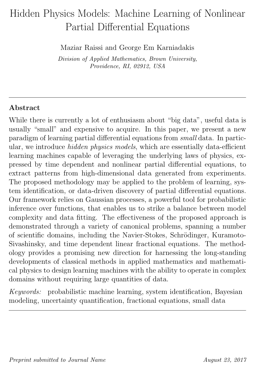
Hidden physics models: Machine learning of nonlinear partial differential equations

Maziar RaissiGeorge Em Karniadakis

article2017Journal of Computational Physics1,360 citations

Introduces hidden physics models, a Gaussian process-based machine learning framework that identifies and discovers governing nonlinear partial differential equations from sparse experimental data.

Listen

Modern engineering and scientific disciplines increasingly rely on data-driven discovery to model complex systems, yet acquiring high-quality, error-free experimental data remains expensive and difficult. Conventional machine learning methods struggle in scenarios where data is scarce relative to the underlying system complexity. The article addresses this challenge by evaluating a new framework termed hidden physics models. The primary objective is to demonstrate that underlying physical laws, expressed as nonlinear partial differential equations, can be directly integrated into probabilistic machine learning to accurately identify unknown system parameters from very small, noisy datasets.

To achieve this, the article utilizes Gaussian processes—a statistical technique for probabilistic inference over functions—to construct multi-output models whose mathematical correlation structures explicitly incorporate discretized physical governing equations. The analysis tests this framework across multiple benchmark physical systems, including fluid dynamics, quantum mechanics, wave propagation, and anomalous diffusion processes, evaluating parameter estimation performance across varying noise levels and observation time intervals using only two temporal snapshots of scattered data.

Across all evaluated scenarios, the methodology successfully recovers true model parameters with high accuracy using minimal data. For example, in fluid flow past a cylinder governed by the Navier-Stokes equations, the algorithm accurately estimates parameters using only 500 scattered data points across two snapshots without requiring direct pressure measurements. Similarly, for the Burgers, Korteweg-de Vries, and Kuramoto-Sivashinsky equations, the method reliably identifies physical parameters using only a few hundred data points—often less than one percent of the datasets required by traditional sparse regression approaches. Furthermore, the model demonstrates the unique ability to infer continuous fractional orders in non-local diffusion processes, while maintaining robustness against moderate observational noise.

These findings indicate that integrating known physical structure into machine learning models substantially lowers data collection costs, eliminates the need for dense sensor grids, and avoids the error accumulation typical of numerical differentiation. For decision-makers, this approach offers a cost-effective pathway to model complex physical assets, calibrate critical parameters, and quantify uncertainties in data-constrained operating environments.

Organizations evaluating this approach should assess whether their engineering problems feature known or partially known physical forms that can be formulated into these probabilistic models. When applying the method, practitioners must ensure measurement snapshots are spaced closely in time to satisfy time-stepping assumptions. Because the computational cost of the model scales cubically with sample size and optimization may encounter local minima, future implementations should incorporate scalable techniques such as variational inference, recursive updates, or fully Bayesian sampling before deploying the models on larger-scale operational systems.

Cover for Hidden physics models: Machine learning of nonlinear partial differential equations

Abstract

While there is currently a lot of enthusiasm about "big data", useful data is usually "small" and expensive to acquire. In this paper, we present a new paradigm of learning partial differential equations from {\em small} data. In particular, we introduce \emph{hidden physics models}, which are essentially data-efficient learning machines capable of leveraging the underlying laws of physics, expressed by time dependent and nonlinear partial differential equations, to extract patterns from high-dimensional data generated from experiments. The proposed methodology may be applied to the problem of learning, system identification, or data-driven discovery of partial differential equations. Our framework relies on Gaussian processes, a powerful tool for probabilistic inference over functions, that enables us to strike a balance between model complexity and data fitting. The effectiveness of the proposed approach is demonstrated through a variety of canonical problems, spanning a number of scientific domains, including the Navier-Stokes, Schrödinger, Kuramoto-Sivashinsky, and time dependent linear fractional equations. The methodology provides a promising new direction for harnessing the long-standing developments of classical methods in applied mathematics and mathematical physics to design learning machines with the ability to operate in complex domains without requiring large quantities of data.

Table of Contents

  • 1 Introduction
  • 2 Problem Setup
  • 3 The Basic Model
  • 4 Learning
  • 5 Results
  • 5.1 Burgers’ Equation
  • 5.2 The KdV Equation
  • 5.3 Kuramoto-Sivashinsky Equation
  • 5.4 Nonlinear Schrödinger Equation
  • 5.5 Navier-Stokes Equations
  • 5.6 Fractional Equations
  • 6 Summary and Discussion
  • References

Knowls

  1. Knowl 1 — Hidden Physics Models for Learning Parametrized Nonlinear Partial Differential Equations

    model/method

    Hidden physics models provide a framework for system identification and parameter estimation of nonlinear partial differential equations (PDEs) from sparse, noisy observations across two time snapshots.

    Consider a parametrized nonlinear PDE defined on a spatial domain Ω⊂RD\Omega \subset \mathbb{R}^D over time t∈[0,T]t \in [0, T]: ht+Nxλh=0h_t + \mathcal{N}_x^\lambda h = 0 where h(t,x)h(t, x) is the latent state, Nxλ\mathcal{N}_x^\lambda is a nonlinear spatial differential operator parametrized by λ∈Rp\lambda \in \mathbb{R}^p, and subscripts denote partial derivatives. Given two observational snapshots {xn−1,hn−1}\{x^{n-1}, h^{n-1}\} and {xn,hn}\{x^n, h^n\} separated by a time step Δt=tn−tn−1\Delta t = t^n - t^{n-1}, applying the backward Euler time stepping scheme gives the discretized system: hn+ΔtNxλhn=hn−1h^n + \Delta t \mathcal{N}_x^\lambda h^n = h^{n-1} where hn(x)=h(tn,x)h^n(x) = h(t^n, x). Linearizing the nonlinear operator on the left-hand side around the state at the previous time step hn−1(x)h^{n-1}(x) yields a linear differential operator Lxλ\mathcal{L}_x^\lambda satisfying: Lxλhn=hn−1\mathcal{L}_x^\lambda h^n = h^{n-1}

    Placing a zero-mean Gaussian process prior on the latent state hn(x)h^n(x): hn(x)∼GP(0,k(x,x′;θ))h^n(x) \sim \mathcal{GP}(0, k(x, x'; \theta)) with covariance kernel k(x,x′;θ)k(x, x'; \theta) (such as a squared exponential kernel with hyperparameters θ\theta), the linearity of Lxλ\mathcal{L}_x^\lambda ensures that hn(x)h^n(x) and hn−1(x)h^{n-1}(x) are jointly distributed as a multi-output Gaussian process: [hnhn−1]∼GP(0,[kn,nkn,n−1kn−1,nkn−1,n−1])\begin{bmatrix} h^n \\ h^{n-1} \end{bmatrix} \sim \mathcal{GP}\left(0, \begin{bmatrix} k^{n,n} & k^{n,n-1} \\ k^{n-1,n} & k^{n-1,n-1} \end{bmatrix}\right) where the constituent covariance functions explicitly encode the physical operator: kn,n(x,x′;θ)=k(x,x′;θ)k^{n,n}(x, x'; \theta) = k(x, x'; \theta) kn,n−1(x,x′;θ,λ)=Lx′λk(x,x′;θ)k^{n,n-1}(x, x'; \theta, \lambda) = \mathcal{L}_{x'}^\lambda k(x, x'; \theta) kn−1,n(x,x′;θ,λ)=Lxλk(x,x′;θ)k^{n-1,n}(x, x'; \theta, \lambda) = \mathcal{L}_x^\lambda k(x, x'; \theta) kn−1,n−1(x,x′;θ,λ)=LxλLx′λk(x,x′;θ)k^{n-1,n-1}(x, x'; \theta, \lambda) = \mathcal{L}_x^\lambda \mathcal{L}_{x'}^\lambda k(x, x'; \theta) The unknown PDE parameters λ\lambda become hyperparameters of the joint covariance functions.

  2. Knowl 2 — Negative Log Marginal Likelihood Objective for Parameter Learning in Hidden Physics Models

    equation

    Given noisy observation vectors hn=hn(xn)+ϵn\mathbf{h}^n = h^n(\mathbf{x}^n) + \boldsymbol{\epsilon}^n and hn−1=hn−1(xn−1)+ϵn−1\mathbf{h}^{n-1} = h^{n-1}(\mathbf{x}^{n-1}) + \boldsymbol{\epsilon}^{n-1} with independent Gaussian measurement noise ϵn,ϵn−1∼N(0,σ2I)\boldsymbol{\epsilon}^n, \boldsymbol{\epsilon}^{n-1} \sim \mathcal{N}(0, \sigma^2 I), the hyperparameters θ\theta of the base kernel, the PDE parameters λ\lambda, and the noise variance σ2\sigma^2 are estimated by minimizing the negative log marginal likelihood: −log⁡p(h∣θ,λ,σ2)=12hTK−1h+12log⁡∣K∣+N2log⁡(2π)-\log p(\mathbf{h} \mid \theta, \lambda, \sigma^2) = \frac{1}{2} \mathbf{h}^T K^{-1} \mathbf{h} + \frac{1}{2} \log |K| + \frac{N}{2} \log(2\pi) where h=[hnhn−1]∈RN\mathbf{h} = \begin{bmatrix} \mathbf{h}^n \\ \mathbf{h}^{n-1} \end{bmatrix} \in \mathbb{R}^N is the concatenated observation vector of total length N=Nn+Nn−1N = N_n + N_{n-1}, and the full dense covariance matrix K∈RN×NK \in \mathbb{R}^{N \times N} is defined by: K=[kn,n(xn,xn)kn,n−1(xn,xn−1)kn−1,n(xn−1,xn)kn−1,n−1(xn−1,xn−1)]+σ2IK = \begin{bmatrix} k^{n,n}(\mathbf{x}^n, \mathbf{x}^n) & k^{n,n-1}(\mathbf{x}^n, \mathbf{x}^{n-1}) \\ k^{n-1,n}(\mathbf{x}^{n-1}, \mathbf{x}^n) & k^{n-1,n-1}(\mathbf{x}^{n-1}, \mathbf{x}^{n-1}) \end{bmatrix} + \sigma^2 I Optimization is performed via the quasi-Newton L-BFGS optimizer.

    The objective function incorporates an automatic complexity regularizer: the quadratic data-fit term 12hTK−1h\frac{1}{2}\mathbf{h}^T K^{-1}\mathbf{h} rewards matching observations, while the log-determinant term 12log⁡∣K∣\frac{1}{2}\log |K| penalizes model complexity, adhering to Occam's razor principle and preventing overfitting even when trained on small datasets.

  3. Knowl 3 — Hidden Physics Model for Incompressible Navier-Stokes Equations without Pressure Measurements

    model/method

    For the two-dimensional incompressible Navier-Stokes equations: ut+λ1(uux+vuy)=−px+λ2(uxx+uyy)u_t + \lambda_1 (u u_x + v u_y) = -p_x + \lambda_2 (u_{xx} + u_{yy}) vt+λ1(uvx+vvy)=−py+λ2(vxx+vyy)v_t + \lambda_1 (u v_x + v v_y) = -p_y + \lambda_2 (v_{xx} + v_{yy}) with unknown parameters λ=(λ1,λ2)\lambda = (\lambda_1, \lambda_2) and divergence-free condition ux+vy=0u_x + v_y = 0, the velocity field is represented via a latent stream function ψn(x,y)\psi^n(x, y) such that: un=ψyn,vn=−ψxnu^n = \psi_y^n, \quad v^n = -\psi_x^n which identically satisfies incompressibility.

    Placing independent zero-mean Gaussian process priors on ψn(x,y)∼GP(0,k((x,y),(x′,y′);θ))\psi^n(x, y) \sim \mathcal{GP}(0, k((x, y), (x', y'); \theta)) and the pressure field pn(x,y)∼GP(0,kp,pn,n((x,y),(x′,y′);θp))p^n(x, y) \sim \mathcal{GP}(0, k_{p,p}^{n,n}((x, y), (x', y'); \theta_p)) yields a prior over velocity components with kernel entries: ku,un,n=∂2k∂y∂y′,ku,vn,n=−∂2k∂y∂x′,kv,un,n=−∂2k∂x∂y′,kv,vn,n=∂2k∂x∂x′k_{u,u}^{n,n} = \frac{\partial^2 k}{\partial y \partial y'}, \quad k_{u,v}^{n,n} = -\frac{\partial^2 k}{\partial y \partial x'}, \quad k_{v,u}^{n,n} = -\frac{\partial^2 k}{\partial x \partial y'}, \quad k_{v,v}^{n,n} = \frac{\partial^2 k}{\partial x \partial x'} Linearizing the backward Euler discretization around previous velocity states (un−1,vn−1)(u^{n-1}, v^{n-1}) gives: L(x,y)λun+Δt pxn=un−1,L(x,y)λvn+Δt pyn=vn−1\mathcal{L}_{(x,y)}^\lambda u^n + \Delta t \, p_x^n = u^{n-1}, \quad \mathcal{L}_{(x,y)}^\lambda v^n + \Delta t \, p_y^n = v^{n-1} where the linear operator is defined by: L(x,y)λh:=h+Δtλ1(un−1hx+vn−1hy)−Δtλ2(hxx+hyy)\mathcal{L}_{(x,y)}^\lambda h := h + \Delta t \lambda_1 (u^{n-1} h_x + v^{n-1} h_y) - \Delta t \lambda_2 (h_{xx} + h_{yy})

    This yields a 5-output Gaussian process over [un,vn,pn,un−1,vn−1]T[u^n, v^n, p^n, u^{n-1}, v^{n-1}]^T with cross-covariance blocks: ku,un,n−1=L(x′,y′)λku,un,n,ku,vn,n−1=L(x′,y′)λku,vn,nk_{u,u}^{n,n-1} = \mathcal{L}_{(x',y')}^\lambda k_{u,u}^{n,n}, \quad k_{u,v}^{n,n-1} = \mathcal{L}_{(x',y')}^\lambda k_{u,v}^{n,n} kv,un,n−1=L(x′,y′)λkv,un,n,kv,vn,n−1=L(x′,y′)λkv,vn,nk_{v,u}^{n,n-1} = \mathcal{L}_{(x',y')}^\lambda k_{v,u}^{n,n}, \quad k_{v,v}^{n,n-1} = \mathcal{L}_{(x',y')}^\lambda k_{v,v}^{n,n} kp,un,n−1=Δt∂∂x′kp,pn,n,kp,vn,n−1=Δt∂∂y′kp,pn,nk_{p,u}^{n,n-1} = \Delta t \frac{\partial}{\partial x'} k_{p,p}^{n,n}, \quad k_{p,v}^{n,n-1} = \Delta t \frac{\partial}{\partial y'} k_{p,p}^{n,n} ku,un−1,n−1=L(x,y)λku,un,n−1+Δt∂∂xkp,un,n−1k_{u,u}^{n-1,n-1} = \mathcal{L}_{(x,y)}^\lambda k_{u,u}^{n,n-1} + \Delta t \frac{\partial}{\partial x} k_{p,u}^{n,n-1} ku,vn−1,n−1=L(x,y)λku,vn,n−1+Δt∂∂xkp,vn,n−1k_{u,v}^{n-1,n-1} = \mathcal{L}_{(x,y)}^\lambda k_{u,v}^{n,n-1} + \Delta t \frac{\partial}{\partial x} k_{p,v}^{n,n-1} kv,vn−1,n−1=L(x,y)λkv,vn,n−1+Δt∂∂ykp,vn,n−1k_{v,v}^{n-1,n-1} = \mathcal{L}_{(x,y)}^\lambda k_{v,v}^{n,n-1} + \Delta t \frac{\partial}{\partial y} k_{p,v}^{n,n-1} Because pressure pnp^n is modeled as a latent variable, the PDE parameters (λ1,λ2)(\lambda_1, \lambda_2) can be inferred exclusively from sparse velocity field data without requiring pressure or vorticity measurements.

  4. Knowl 4 — Hidden Physics Model for Fractional Differential Equations via Fourier Transform Kernels

    model/method

    Hidden physics models can infer non-integer fractional derivative orders directly from data. Consider the one-dimensional fractional PDE: ut−λ1D−∞,xλ2u=0u_t - \lambda_1 \mathcal{D}_{-\infty,x}^{\lambda_2} u = 0 where D−∞,xλ2\mathcal{D}_{-\infty,x}^{\lambda_2} is the Riemann-Liouville fractional derivative of unknown real order λ2∈R\lambda_2 \in \mathbb{R}, and λ1\lambda_1 is an unknown parameter. Applying backward Euler discretization gives: un−Δtλ1D−∞,xλ2un=un−1u^n - \Delta t \lambda_1 \mathcal{D}_{-\infty,x}^{\lambda_2} u^n = u^{n-1}

    Placing a Gaussian process prior un(x)∼GP(0,k(x,x′;θ))u^n(x) \sim \mathcal{GP}(0, k(x, x'; \theta)) induces a joint GP over [un,un−1]T[u^n, u^{n-1}]^T. The cross-covariance kernel kn,n−1(x,x′;θ,λ1,λ2)k^{n,n-1}(x, x'; \theta, \lambda_1, \lambda_2) is obtained analytically via the inverse Fourier transform of the operator applied to the kernel Fourier transform k^(w,w′;θ)\hat{k}(w, w'; \theta): kn,n−1(x,x′;θ,λ1,λ2)=F−1{[1−Δtλ1(−iw′)λ2]k^(w,w′;θ)}k^{n,n-1}(x, x'; \theta, \lambda_1, \lambda_2) = \mathcal{F}^{-1}\left\{ [1 - \Delta t \lambda_1 (-i w')^{\lambda_2}] \hat{k}(w, w'; \theta) \right\} Kernels kn−1,nk^{n-1,n} and kn−1,n−1k^{n-1,n-1} are obtained analogously.

    Similarly, for diffusion governed by the fractional Laplacian (−∇xα)(-\nabla_x^\alpha): ut+(−∇xα)u=0u_t + (-\nabla_x^\alpha) u = 0 whose Fourier symbol is ∣w∣α|w|^\alpha, the kernel Fourier representation uses ∣w∣αu^(w)|w|^\alpha \hat{u}(w). This enables direct data-driven discovery of the fractional index α\alpha characterizing non-local interactions and α\alpha-stable Lévy processes.

  5. Knowl 5 — Parameter Identification in 1D Nonlinear PDEs (Burgers, KdV, and Kuramoto-Sivashinsky)

    empirical result

    The hidden physics model framework was benchmarked on parameter discovery for three canonical 1D nonlinear PDEs using only two time snapshots:

    1. Burgers' Equation (ut+λ1uux−λ2uxx=0u_t + \lambda_1 u u_x - \lambda_2 u_{xx} = 0, true values λ1=1.0,λ2=0.1\lambda_1 = 1.0, \lambda_2 = 0.1): Trained on 140 randomly chosen points (71 points at t=8.10t = 8.10 and 69 points at t=8.20t = 8.20, Δt=0.1\Delta t = 0.1) out of 25,856 points in the original dataset. On clean data, the identified PDE was ut+1.028uux−0.101uxx=0u_t + 1.028 u u_x - 0.101 u_{xx} = 0. With 1% Gaussian noise, the identified PDE was ut+1.017uux−0.094uxx=0u_t + 1.017 u u_x - 0.094 u_{xx} = 0.

    2. Korteweg-de Vries (KdV) Equation (ut+λ1uux+λ2uxxx=0u_t + \lambda_1 u u_x + \lambda_2 u_{xxx} = 0, true values λ1=6.0,λ2=1.0\lambda_1 = 6.0, \lambda_2 = 1.0): Trained on 220 points (111 points at t=16.20t = 16.20 and 109 points at t=16.30t = 16.30, Δt=0.1\Delta t = 0.1) out of 102,912 points. On clean data, the identified PDE was ut+6.115uux+1.047uxxx=0u_t + 6.115 u u_x + 1.047 u_{xxx} = 0. With 1% noise, the identified PDE was ut+5.722uux+0.958uxxx=0u_t + 5.722 u u_x + 0.958 u_{xxx} = 0.

    3. Kuramoto-Sivashinsky Equation (ut+λ1uux+λ2uxx+λ3uxxxx=0u_t + \lambda_1 u u_x + \lambda_2 u_{xx} + \lambda_3 u_{xxxx} = 0, true values λ1=1.0,λ2=1.0,λ3=1.0\lambda_1 = 1.0, \lambda_2 = 1.0, \lambda_3 = 1.0): Trained on 600 points (301 points at t=81.20t = 81.20 and 299 points at t=81.60t = 81.60, Δt=0.4\Delta t = 0.4) out of 257,024 points. On clean data, the identified PDE was ut+0.952uux+1.005uxx+0.980uxxxx=0u_t + 0.952 u u_x + 1.005 u_{xx} + 0.980 u_{xxxx} = 0. With 1% noise, the identified PDE was ut+0.908uux+0.951uxx+0.927uxxxx=0u_t + 0.908 u u_x + 0.951 u_{xx} + 0.927 u_{xxxx} = 0.

  6. Knowl 6 — Hidden Physics Model Formulation and Parameter Discovery for Nonlinear Schrödinger Equation

    model/method

    The 1D cubic nonlinear Schrödinger equation is given by: iht+λ1hxx+λ2∣h∣2h=0i h_t + \lambda_1 h_{xx} + \lambda_2 |h|^2 h = 0 with true parameters λ1=0.5,λ2=1.0\lambda_1 = 0.5, \lambda_2 = 1.0. Expressing the complex state as h=u+ivh = u + iv gives the coupled system: ut+λ1vxx+λ2(u2+v2)v=0u_t + \lambda_1 v_{xx} + \lambda_2 (u^2 + v^2) v = 0 vt−λ1uxx−λ2(u2+v2)u=0v_t - \lambda_1 u_{xx} - \lambda_2 (u^2 + v^2) u = 0

    Applying backward Euler time discretization and linearizing about the previous state (un−1,vn−1)(u^{n-1}, v^{n-1}) yields: un+Δtλ1vxxn+Δtλ2[(un−1)2+(vn−1)2]vn=un−1u^n + \Delta t \lambda_1 v_{xx}^n + \Delta t \lambda_2 [(u^{n-1})^2 + (v^{n-1})^2] v^n = u^{n-1} vn−Δtλ1uxxn−Δtλ2[(un−1)2+(vn−1)2]un=vn−1v^n - \Delta t \lambda_1 u_{xx}^n - \Delta t \lambda_2 [(u^{n-1})^2 + (v^{n-1})^2] u^n = v^{n-1}

    Placing independent Gaussian process priors un(x)∼GP(0,ku(x,x′;θu))u^n(x) \sim \mathcal{GP}(0, k_u(x, x'; \theta_u)) and vn(x)∼GP(0,kv(x,x′;θv))v^n(x) \sim \mathcal{GP}(0, k_v(x, x'; \theta_v)) creates a 4-output Gaussian process for [un,vn,un−1,vn−1]T[u^n, v^n, u^{n-1}, v^{n-1}]^T.

    When evaluated on 100 points (49 points at t=2.55726t = 2.55726 and 51 points at t=2.56354t = 2.56354, Δt=0.0063\Delta t = 0.0063) out of 256,512 points in the dataset:

    • Clean data identified iht+0.506hxx+0.995∣h∣2h=0i h_t + 0.506 h_{xx} + 0.995 |h|^2 h = 0 (median over all pairs: λ1=0.5009,λ2=1.0001\lambda_1 = 0.5009, \lambda_2 = 1.0001).
    • 1% noise data identified iht+0.476hxx+0.999∣h∣2h=0i h_t + 0.476 h_{xx} + 0.999 |h|^2 h = 0 (median over all pairs: λ1=0.4713,λ2=0.9946\lambda_1 = 0.4713, \lambda_2 = 0.9946).
  7. Knowl 7 — Parameter Discovery in 2D Navier-Stokes Flow Past a Cylinder from Sparse Velocity Snapshots

    empirical result

    The hidden physics model framework was applied to two-dimensional incompressible flow past a circular cylinder at Reynolds number Re=100Re = 100 simulated via the Immersed Boundary Projection Method. The nondimensionalized Navier-Stokes equations have true convective parameter λ1=1.0\lambda_1 = 1.0 and diffusion parameter λ2=1/Re=0.01\lambda_2 = 1/Re = 0.01: ut+λ1(uux+vuy)=−px+λ2(uxx+uyy)u_t + \lambda_1(u u_x + v u_y) = -p_x + \lambda_2(u_{xx} + u_{yy}) vt+λ1(uvx+vvy)=−py+λ2(vxx+vyy)v_t + \lambda_1(u v_x + v v_y) = -p_y + \lambda_2(v_{xx} + v_{yy})

    Using only 500 scattered velocity measurements across two snapshots (251251 points at t=0.18t = 0.18 and 249249 points at t=0.20t = 0.20, Δt=0.02\Delta t = 0.02) without any pressure or vorticity observations:

    • On clean data, the identified parameters for a representative pair were λ1=0.983\lambda_1 = 0.983 and λ2=0.00826\lambda_2 = 0.00826 (across 501 consecutive pairs, median values were λ1=0.9928,λ2=0.0077\lambda_1 = 0.9928, \lambda_2 = 0.0077).
    • Under 1% Gaussian noise, the identified parameters for the representative pair were λ1=0.849\lambda_1 = 0.849 and λ2=0.01399\lambda_2 = 0.01399 (median values across 501 pairs were λ1=0.8717,λ2=0.0063\lambda_1 = 0.8717, \lambda_2 = 0.0063).
    • Under 5% Gaussian noise, the median estimates across 501 pairs were λ1=0.6498\lambda_1 = 0.6498 and λ2=0.0030\lambda_2 = 0.0030.
  8. Knowl 8 — Parameter Estimation Statistics across Consecutive Snapshots and Noise Levels

    data/table

    Statistical distributions (first quartile, median, third quartile) of estimated PDE parameters obtained by fitting hidden physics models to every pair of consecutive snapshots in benchmark datasets under varying noise levels demonstrate accuracy and noise sensitivity:

    Burgers' Eq. Clean Data 1% Noise 5% Noise
    λ1\lambda_1 λ2\lambda_2 λ1\lambda_1 λ2\lambda_2 λ1\lambda_1 λ2\lambda_2
    First Quartile 1.0247 0.0942 0.9168 0.0784 0.3135 0.0027
    Median 1.0379 0.0976 1.0274 0.0919 0.8294 0.0981
    Third Quartile 1.0555 0.0987 1.1161 0.1166 1.2488 0.1543
    KdV Eq. Clean Data 1% Noise 5% Noise
    λ1\lambda_1 λ2\lambda_2 λ1\lambda_1 λ2\lambda_2 λ1\lambda_1 λ2\lambda_2
    First Quartile 5.7783 0.9299 5.3358 0.7885 3.7435 0.2280
    Median 5.8920 0.9656 5.5757 0.8777 4.5911 0.6060
    Third Quartile 6.0358 1.0083 5.7840 0.9491 5.5106 0.8407
    Navier-Stokes Clean Data 1% Noise 5% Noise
    λ1\lambda_1 λ2\lambda_2 λ1\lambda_1 λ2\lambda_2 λ1\lambda_1 λ2\lambda_2
    First Quartile 0.9854 0.0069 0.8323 0.0057 0.5373 0.0026
    Median 0.9928 0.0077 0.8717 0.0063 0.6498 0.0030
    Third Quartile 1.0001 0.0086 0.9102 0.0070 0.7619 0.0046

    For Burgers' equation (true λ1=1.0,λ2=0.1\lambda_1 = 1.0, \lambda_2 = 0.1), KdV equation (true λ1=6.0,λ2=1.0\lambda_1 = 6.0, \lambda_2 = 1.0), and Navier-Stokes equations (true λ1=1.0,λ2=0.01\lambda_1 = 1.0, \lambda_2 = 0.01), median values remain closely aligned with ground truth parameters under clean data and 1% noise. As noise increases to 5%, estimation variance increases substantially and median values exhibit systematic bias, reflecting decreased identification confidence.

  9. Knowl 9 — Discovery of Fractional Differential Equations from Stochastic Particle Trajectories

    empirical result

    Hidden physics models successfully identified continuous and fractional differential equations from displacement histograms of simulated stochastic processes:

    1. Brownian Motion: For particle position simulated with increments x(t+Δt)∼N(x(t),Δt)x(t + \Delta t) \sim \mathcal{N}(x(t), \Delta t), the associated Fokker-Planck equation is the standard diffusion equation ut=0.5uxxu_t = 0.5 u_{xx}. Using two displacement histograms with 100 bins each separated by Δt=0.01\Delta t = 0.01, the hidden physics model identified: ut−0.513D−∞,x2.016u=0u_t - 0.513 \mathcal{D}_{-\infty,x}^{2.016} u = 0 recovering the true diffusion coefficient (0.513≈0.50.513 \approx 0.5) and the fractional derivative order (2.016≈2.02.016 \approx 2.0, corresponding to standard diffusion).

    2. α\alpha-Stable Lévy Process: For an α\alpha-stable Lévy process whose generator is the fractional Laplacian (−∇xα)(-\nabla_x^\alpha), using two 100-bin displacement histograms separated by Δt=0.01\Delta t = 0.01 and the model ut+(−∇xα)u=0u_t + (-\nabla_x^\alpha) u = 0, the algorithm identified the fractional order as: ut+(−∇x1.413)u=0u_t + (-\nabla_x^{1.413}) u = 0 This validates the method's ability to discover real-valued non-integer differential operators without pre-specifying integer derivative candidates.

  10. Knowl 10 — Computational and Methodological Limitations of Hidden Physics Models

    limitation

    Hidden physics models have several computational and theoretical limitations:

    1. Cubic Computational Scaling: Minimizing the negative log marginal likelihood requires inverting dense covariance matrices K∈RN×NK \in \mathbb{R}^{N \times N}, scaling cubically as O(N3)\mathcal{O}(N^3) in time and O(N2)\mathcal{O}(N^2) in memory with the total number of observation points NN.

    2. Time Discretization and Linearization Errors: The framework assumes the time gap Δt\Delta t between snapshots is small enough for backward Euler time stepping and linearization around the previous snapshot state to hold. Increasing Δt\Delta t introduces substantial discretization errors (e.g., in Burgers' equation, parameter estimates degrade from λ1=1.0283,λ2=0.1009\lambda_1 = 1.0283, \lambda_2 = 0.1009 at Δt=0.1\Delta t = 0.1 to λ1=1.2960,λ2=0.0431\lambda_1 = 1.2960, \lambda_2 = 0.0431 at Δt=1.5\Delta t = 1.5).

    3. Noise Sensitivity at Small Δt\Delta t: While small Δt\Delta t reduces discretization bias, it increases susceptibility to measurement noise when computing temporal differences between snapshots.

    4. Optimization Landscapes: The negative log marginal likelihood is non-convex and lacks theoretical guarantees against local minima during optimization.

Coverage note — None was omitted; all contributed methodology, equation formulations, benchmark PDE results, fractional equation discovery, and limitation analyses have been captured.

References

  1. 1.M. Raissi, P. Perdikaris, G. E. Karniadakis, Numerical gaussian processes for time-dependent and non-linear partial differential equations, arXiv preprint arXiv:1703.10230 (2017).
  2. 2.S. H. Rudy, S. L. Brunton, J. L. Proctor, J. N. Kutz, Data-driven discovery of partial differential equations, Science Advances 3 (2017).
  3. 3.M. Raissi, P. Perdikaris, G. E. Karniadakis, Inferring solutions of differential equations using noisy multi-fidelity data, Journal of Computational Physics 335 (2017) 736 – 746.
  4. 4.M. Raissi, P. Perdikaris, G. E. Karniadakis, Machine learning of linear differential equations using gaussian processes, Journal of Computational Physics 348 (2017) 683 – 693.
  5. 5.C. E. Rasmussen, C. K. Williams, Gaussian processes for machine learning, volume 1, MIT press Cambridge, 2006.
  6. 6.K. P. Murphy, Machine learning: a probabilistic perspective, MIT press, 2012.
  7. 7.R. M. Neal, Bayesian learning for neural networks, volume 118, Springer Science & Business Media, 2012.
  8. 8.V. Vapnik, The nature of statistical learning theory, Springer Science & Business Media, 2013.
  9. 9.B. Sch¨olkopf, A. J. Smola, Learning with kernels: support vector machines, regularization, optimization, and beyond, MIT press, 2002.
  10. 10.M. E. Tipping, Sparse Bayesian learning and the relevance vector machine, The journal of machine learning research 1 (2001) 211–244.
  11. 11.A. Tikhonov, Solution of incorrectly formulated problems and the regularization method, in: Soviet Math. Dokl., volume 5, pp. 1035–1038.
  12. 12.A. N. Tikhonov, V. Y. Arsenin, Solutions of Ill-posed problems, W.H. Winston, 1977.
  13. 13.T. Poggio, F. Girosi, Networks for approximation and learning, Proceedings of the IEEE 78 (1990) 1481–1497.
  14. 14.N. Aronszajn, Theory of reproducing kernels, Transactions of the American Mathematical Society 68 (1950) 337–404.
  15. 15.S. Saitoh, Theory of reproducing kernels and its applications, volume 189, Longman, 1988.
  16. 16.A. Berlinet, C. Thomas-Agnan, Reproducing kernel Hilbert spaces in probability and statistics, Springer Science & Business Media, 2011.
  17. 17.D. Duvenaud, J. R. Lloyd, R. Grosse, J. B. Tenenbaum, Z. Ghahramani, Structure discovery in nonparametric regression through compositional kernel search, arXiv preprint arXiv:1302.4922 (2013).
  18. 18.R. Grosse, R. R. Salakhutdinov, W. T. Freeman, J. B. Tenenbaum, Exploiting compositionality to explore a large space of model structures, arXiv preprint arXiv:1210.4856 (2012).
  19. 19.G. Malkomes, C. Schaff, R. Garnett, Bayesian optimization for automated model selection, in: Advances in Neural Information Processing Systems, pp. 2900–2908.
  20. 20.R. Calandra, J. Peters, C. E. Rasmussen, M. P. Deisenroth, Manifold Gaussian processes for regression, in: Neural Networks (IJCNN), 2016 International Joint Conference on, IEEE, pp. 3338–3345.
  21. 21.M. Raissi, G. Karniadakis, Deep multi-fidelity Gaussian processes, arXiv preprint arXiv:1604.07484 (2016).
  22. 22.D. C. Liu, J. Nocedal, On the limited memory BFGS method for large scale optimization, Mathematical programming 45 (1989) 503–528.
  23. 23.C. E. Rasmussen, Z. Ghahramani, Occam’s razor, Advances in neural information processing systems (2001) 294–300.
  24. 24.S. L. Brunton, J. L. Proctor, J. N. Kutz, Discovering governing equations from data by sparse identification of nonlinear dynamical systems, Proceedings of the National Academy of Sciences 113 (2016) 3932–3937.
  25. 25.A. M. Stuart, Inverse problems: a Bayesian perspective, Acta Numerica 19 (2010) 451–559.
  26. 26.E. Snelson, Z. Ghahramani, Sparse Gaussian processes using pseudo-inputs, in: Advances in neural information processing systems, pp. 1257–1264.
  27. 27.J. Hensman, N. Fusi, N. D. Lawrence, Gaussian processes for big data, in: Proceedings of the Twenty-Ninth Conference on Uncertainty in Artificial Intelligence, UAI 2013, Bellevue, WA, USA, August 11-15, 2013.
  28. 28.M. Raissi, Parametric gaussian process regression for big data, arXiv preprint arXiv:1704.03144 (2017).
  29. 29.C. Basdevant, M. Deville, P. Haldenwang, J. Lacroix, J. Ouazzani, R. Peyret, P. Orlandi, A. Patera, Spectral and finite difference solutions of the Burgers equation, Computers & fluids 14 (1986) 23–41.
  30. 30.T. Dauxois, Fermi, Pasta, Ulam and a mysterious lady, arXiv preprint arXiv:0801.1590 (2008).
  31. 31.J. M. Hyman, B. Nicolaenko, The Kuramoto-Sivashinsky equation: a bridge between pde’s and dynamical systems, Physica D: Nonlinear Phenomena 18 (1986) 113–126.
  32. 32.B. I. Shraiman, Order, disorder, and phase turbulence, Physical review letters 57 (1986) 325.
  33. 33.B. Nicolaenko, B. Scheurer, R. Temam, Some global dynamical properties of the Kuramoto-Sivashinsky equations: nonlinear stability and attractors, Physica D: Nonlinear Phenomena 16 (1985) 155–183.
  34. 34.J. N. Kutz, S. L. Brunton, B. W. Brunton, J. L. Proctor, Dynamic Mode Decomposition: Data-Driven Modeling of Complex Systems, volume 149, SIAM, 2016.
  35. 35.K. Taira, T. Colonius, The immersed boundary method: a projection approach, Journal of Computational Physics 225 (2007) 2118–2137.
  36. 36.T. Colonius, K. Taira, A fast immersed boundary method using a nullspace approach and multi-domain far-field boundary conditions, Computer Methods in Applied Mechanics and Engineering 197 (2008) 2131–2146.
  37. 37.I. Podlubny, Fractional differential equations: an introduction to fractional derivatives, fractional differential equations, to methods of their solution and some of their applications, volume 198, Academic press, 1998.
  38. 38.J. Nolan, Stable distributions: models for heavy-tailed data, Birkhauser New York, 2003.
  39. 39.J. M. Chambers, C. L. Mallows, B. Stuck, A method for simulating stable random variables, Journal of the american statistical association 71 (1976) 340–344.
  40. 40.A. Weron, R. Weron, Computer simulation of l´evy α-stable variables and processes, ChaosThe Interplay Between Stochastic and Deterministic Behaviour (1995) 379–392.
  41. 41.J. Hartikainen, S. S¨arkk¨a, Kalman filtering and smoothing solutions to temporal Gaussian process regression models, in: Machine Learning for Signal Processing (MLSP), 2010 IEEE International Workshop on, IEEE, pp. 379–384.

Citation

MLA
Raissi, M., and G. E. Karniadakis. “Hidden Physics Models: Machine Learning of Nonlinear Partial Differential Equations”. Journal of Computational Physics, vol. 357, 2018, pp. 125–41, https://doi.org/10.1016/j.jcp.2017.11.039.
APA
Raissi, M., & Karniadakis, G. E. (2018). Hidden physics models: Machine learning of nonlinear partial differential equations. Journal of Computational Physics, 357, 125–141. https://doi.org/10.1016/j.jcp.2017.11.039
Chicago
Raissi, M., and G. E. Karniadakis. 2018. “Hidden Physics Models: Machine Learning of Nonlinear Partial Differential Equations”. Journal of Computational Physics 357: 125–41. https://doi.org/10.1016/j.jcp.2017.11.039.
Harvard
Raissi, M. and Karniadakis, G.E. (2018) “Hidden physics models: Machine learning of nonlinear partial differential equations”, Journal of Computational Physics, 357, pp. 125–141. Available at: https://doi.org/10.1016/j.jcp.2017.11.039.
Vancouver
1. Raissi M, Karniadakis GE (2018) Hidden physics models: Machine learning of nonlinear partial differential equations. Journal of Computational Physics 357:125–141

BibTeX

@article{Raissi_2018, title={Hidden physics models: Machine learning of nonlinear partial differential equations}, volume={357}, ISSN={0021-9991}, url={http://dx.doi.org/10.1016/j.jcp.2017.11.039}, DOI={10.1016/j.jcp.2017.11.039}, journal={Journal of Computational Physics}, publisher={Elsevier BV}, author={Raissi, Maziar and Karniadakis, George Em}, year={2018}, month=Mar, pages={125–141} }
Metadata:Crossref

Source Code

This paper has an official code repository available. Click below to access the source code.

View Repository

Access the Paper

This paper is available from its original source. Click below to access the PDF.

Open PDF