Neural Operator: Learning Maps Between Function Spaces With Applications to PDEs

Nikola KovachkiZongyi LiBurigede LiuKamyar AzizzadenesheliKaushik BhattacharyaAndrew StuartAnima Anandkumar

article2023JMLR1,053 citations

Proposes neural operators to learn mappings directly between infinite-dimensional function spaces, establishing a discretization-invariant framework with universal approximation guarantees that solves complex partial differential equations orders of magnitude faster than traditional numerical solvers.

Listen

Simulating complex physical systems governed by partial differential equations—such as fluid turbulence, subsurface flow, and structural deformation—is essential across engineering and scientific disciplines. Conventional numerical solvers are computationally expensive, often taking hours or days to run, which makes large-scale parameter studies, design optimization, and real-time predictions impractical. While standard deep learning methods have been applied as surrogate models to speed up these simulations, they are tied to fixed grid resolutions and cannot easily generalize when mesh geometry or resolution changes without being retrained.

The objective of the article is to introduce and evaluate neural operators, a deep learning framework designed to learn mappings between infinite-dimensional function spaces rather than finite-dimensional vectors. The authors evaluate whether these architectures can provide accurate, resolution-invariant surrogate models for partial differential equations while achieving dramatic speedups over traditional numerical solvers.

To achieve this, the authors develop a general neural operator framework that composes linear integral kernel operators with non-linear activation functions. They implement and benchmark four efficient parameterizations: Graph Neural Operators, Low-Rank Neural Operators, Multipole Graph Neural Operators, and Fourier Neural Operators. The models were tested on classic benchmark equations representing diverse physical regimes: one-dimensional Poisson and Burgers' equations, two-dimensional Darcy subsurface flow, and two-dimensional incompressible Navier-Stokes equations modeling fluid dynamics. The evaluation compared the proposed models against standard neural networks, convolutional networks, and competing operator architectures across varying mesh resolutions and noise levels, as well as in downstream applications like Bayesian inverse problems.

The analysis yields several key findings. First, neural operators are fundamentally discretization-invariant; a model trained on a coarse mesh can be evaluated directly on a much finer mesh—enabling zero-shot super-resolution—while keeping prediction error virtually constant. Second, the Fourier Neural Operator consistently outperformed existing machine learning methods, achieving relative errors under 1% on the Darcy flow problem and Burgers' equation, and under 1% for Navier-Stokes flow at lower Reynolds numbers and around 8% at higher Reynolds numbers. Third, in terms of speed, the Fourier Neural Operator evaluated Navier-Stokes instances in 0.005 seconds compared to 2.2 seconds for a standard pseudo-spectral solver on a 256 by 256 grid. In an end-to-end Bayesian inverse sampling workflow, this reduced total run time from over 18 hours to approximately 2.5 minutes while matching the traditional solver's posterior accuracy. Fourth, testing demonstrated that neural operators maintain stability against input noise, especially when noise is included during training.

These findings indicate that neural operators can substantially lower computational costs, accelerate research and development timelines, and enable near-real-time decision-making in engineering workflows that rely heavily on physical simulations. Because the models learn the underlying continuum operators rather than grid-specific patterns, engineering teams can train surrogate models once on low-resolution or legacy simulation data and deploy them across varying computational grids without retraining or losing accuracy.

Organizations evaluating neural operators should consider adopting Fourier Neural Operators for problems defined on regular geometries where speed is paramount, while using graph-based neural operators for irregular geometries or complex unstructured meshes. Teams should incorporate data augmentation, such as training with noise, to enhance model robustness for applications with steep gradients or experimental measurement errors. Before deploying these models into mission-critical engineering pipelines, organizations should conduct pilot validations to account for limitations in non-smoothing problems with sharp discontinuities, assess training data requirements for high-Reynolds-number turbulent regimes, and verify the surrogate's accuracy boundaries against traditional high-fidelity solvers.

California Institute of Technology NVIDIA University of Cambridge fourier neural networks parameterization neural operator operator learning function spaces

arXiv: 2108.08481 neuraloperator/neuraloperator

Paper: Fourier Neural Operator for Parametric Partial Differential Equations, Zongyi Li et al. (2020). This paper establishes the Fourier Neural Operator architecture for mapping between function spaces in parametric PDEs, providing the core spectral formulation that the source generalizes and synthesizes.
Paper: Learning nonlinear operators via DeepONet based on the universal approximation theorem of operators, Lu Lu et al. (2021). This paper establishes the foundational DeepONet architecture and operator universal approximation framework for learning maps between function spaces, serving as a primary benchmark and precursor to neural operators.
Paper: Geometric Deep Learning: Going beyond Euclidean data, Michael M. Bronstein et al. (2016). This survey establishes the foundations of spatial and spectral kernel operations on non-Euclidean geometries, providing essential background for graph neural operator parameterizations.
Paper: Approximation by Superpositions of a Sigmoidal Function, George Cybenko (1989). This classic work proves the universal approximation theorem for standard neural networks on finite-dimensional spaces, forming the theoretical baseline that the source generalizes to infinite-dimensional function spaces.
Paper: DGM: A deep learning algorithm for solving partial differential equations, Justin Sirignano et al. (2017). This work introduces mesh-free deep learning for solving partial differential equations, providing context for physics-based machine learning approaches that neural operators improve upon via discretization-invariant operator learning.

Paper: Neural means and kernel corrections for operator learning, Yitzchak Shmalo (2026). This text builds directly on operator learning paradigms like Fourier neural operators by developing hybrid pipelines that combine neural operator means with exact kernel ridge regression corrections.
Paper: KAN: Kolmogorov-Arnold Networks, Ziming Liu et al. (2025). This work extends scientific machine learning for PDEs by replacing standard multilayer perceptron architectures with learnable spline-based Kolmogorov-Arnold Networks.

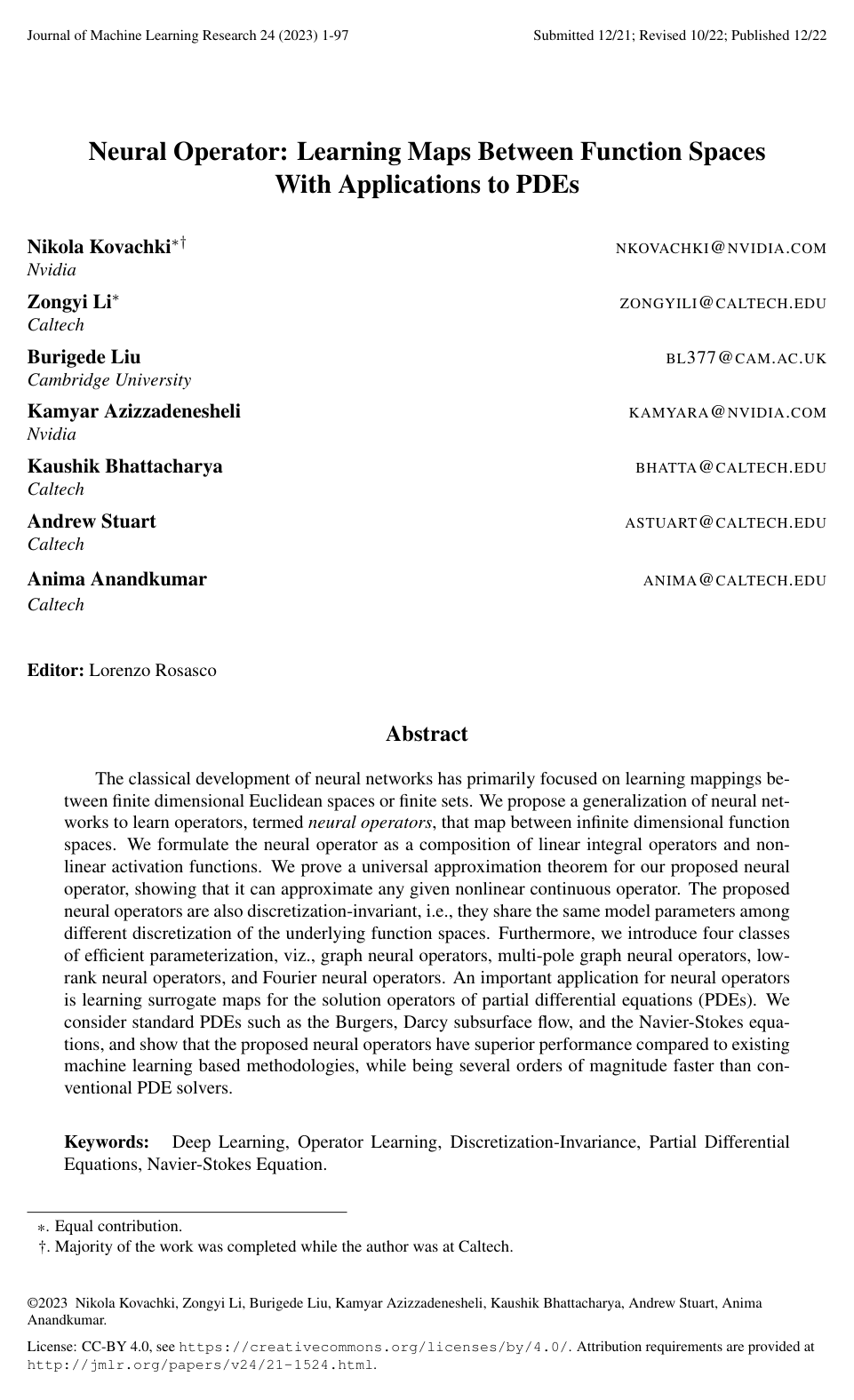
Cover for Neural Operator: Learning Maps Between Function Spaces With Applications to PDEs

Abstract

The classical development of neural networks has primarily focused on learning mappings between finite dimensional Euclidean spaces or finite sets. We propose a generalization of neural networks to learn operators, termed neural operators, that map between infinite dimensional function spaces. We formulate the neural operator as a composition of linear integral operators and non-linear activation functions. We prove a universal approximation theorem for our proposed neural operator, showing that it can approximate any given nonlinear continuous operator. The proposed neural operators are also discretization-invariant, i.e., they share the same model parameters among different discretization of the underlying function spaces. Furthermore, we introduce four classes of efficient parameterization, viz., graph neural operators, multi-pole graph neural operators, low-rank neural operators, and Fourier neural operators. An important application for neural operators is learning surrogate maps for the solution operators of partial differential equations (PDEs). We consider standard PDEs such as the Burgers, Darcy subsurface flow, and the Navier-Stokes equations, and show that the proposed neural operators have superior performance compared to existing machine learning based methodologies, while being several orders of magnitude faster than conventional PDE solvers.

Topics

fourier neural networks parameterization approximation theory diffusion equations ordinary differential equations numerical solution

Keywords

neural operator operator learning function spaces PDE solvers Fourier operators discretization-invariant models Banach space approximation integral operators universal approximation theorems

1. Introduction
1.1 Our Approach
1.2 Background and Context
2. Learning Operators
2.1 Generic Parametric PDEs
2.2 Problem Setting
2.3 Discretization
3. Neural Operators
4. Parameterization and Computation
4.1 Graph Neural Operator (GNO)
4.2 Low-rank Neural Operator (LNO)
4.3 Multipole Graph Neural Operator (MGNO)
4.4 Fourier Neural Operator (FNO)
4.5 Summary
5. Neural Operators and Other Deep Learning Models
5.1 DeepONets
5.2 Transformers as a Special Case of Neural Operators
6. Test Problems
6.1 Poisson Equation
6.2 Darcy Flow
6.3 Burgers’ Equation
6.4 Navier-Stokes Equation
6.4.1 BAYESIAN INVERSE PROBLEM
6.4.2 SPECTRA
6.5 Choice of Loss Criteria
7. Numerical Results
7.1 Poisson Equation
7.2 Darcy and Burgers Equations
7.2.1 DARCY FLOW
7.2.2 BURGERS’ EQUATION
7.2.3 ZERO-SHOT SUPER-RESOLUTION.
7.3 Navier-Stokes Equation
7.3.1 ZERO-SHOT SUPER-RESOLUTION.
7.3.2 SPECTRAL ANALYSIS
7.3.3 NON-PERIODIC BOUNDARY CONDITION.
7.3.4 BAYESIAN INVERSE PROBLEM
7.4 Discussion and Comparison of the Four methods
7.4.1 INGENUITY
7.4.2 EXPRESSIVENESS
7.4.3 COMPLEXITY
7.4.4 REFINABILITY
7.4.5 ROBUSTNESS
8. Literature Review
9. Approximation Theory
9.1 Neural Operators
9.2 Discretization Invariance
9.3 Approximation Theorems
10. Conclusions
10.1 Future Directions
10.1.1 NEW APPLICATIONS
10.1.2 NEW METHODOLOGIES
10.1.3 THEORY
Acknowledgements
References
Appendix A.
Appendix B.
Appendix C.
Appendix D.
Appendix E.
Appendix F.
Appendix G.

Knowls

Knowl 1 — Neural Operator Architecture Framework
model/method
The neural operator generalizes deep neural networks to learn continuous nonlinear maps $G_\theta: \mathcal{A} \to \mathcal{U}$ between infinite-dimensional Banach spaces of functions $\mathcal{A} = C(D; \mathbb{R}^{d_a})$ and $\mathcal{U} = C(D'; \mathbb{R}^{d_u})$ defined on bounded domains $D \subset \mathbb{R}^d$ and $D' \subset \mathbb{R}^{d'}$ .

The architecture is defined by composing local lifting, iterative non-local integral kernel layers, and local projection:

$G_\theta = Q \circ \sigma_T(W_{T-1} + K_{T-1} + b_{T-1}) \circ \dots \circ \sigma_1(W_0 + K_0 + b_0) \circ P$
1. Local Lifting ( $P$ ): The input function $a(x) \in \mathbb{R}^{d_a}$ is pointwise mapped to a higher-dimensional representation $v_0(x) = P(a(x)) \in \mathbb{R}^{d_{v_0}}$ using a local operator (typically a shallow feed-forward network), with $d_{v_0} > d_a$ .
2. Iterative Kernel Integration ( $t = 0, \dots, T-1$ ): Each hidden state $v_t: D_t \to \mathbb{R}^{d_{v_t}}$ is updated to $v_{t+1}: D_{t+1} \to \mathbb{R}^{d_{v_{t+1}}}$ via:
$v_{t+1}(x) = \sigma_{t+1} \left( W_t v_t(\Pi_t(x)) + \int_{D_t} \kappa^{(t)}(x, y) v_t(y) \, d\nu_t(y) + b_t(x) \right) \quad \forall x \in D_{t+1}$

where $\Pi_t: D_{t+1} \to D_t$ is a projection (typically identity when $D_t = D$ ), $W_t \in \mathbb{R}^{d_{v_{t+1}} \times d_{v_t}}$ is a local linear transformation (acting like a residual skip connection), $b_t: D_{t+1} \to \mathbb{R}^{d_{v_{t+1}}}$ is a bias function (often parameterized as a constant vector), $\nu_t$ is a Borel measure on $D_t$ (commonly Lebesgue measure), $\sigma_{t+1}$ is a fixed pointwise activation function, and $\kappa^{(t)}: D_{t+1} \times D_t \to \mathbb{R}^{d_{v_{t+1}} \times d_{v_t}}$ is a continuous kernel function parameterized by neural networks.
1. Local Projection ( $Q$ ): The final hidden state $v_T: D' \to \mathbb{R}^{d_{v_T}}$ is mapped pointwise to the target solution function $u(x) = Q(v_T(x)) \in \mathbb{R}^{d_u}$ .
Parameterized kernel variations include input-dependent kernels $\kappa^{(t)}(x, y, a(x), a(y))$ to propagate parameter influence across deep layers, and state-dependent kernels $\kappa^{(t)}(x, y, v_t(x), v_t(y))$ .
Knowl 2 — Mathematical Formulation of Discretization Invariance
definition
Let $D \subset \mathbb{R}^d$ be a bounded domain, and let $\mathcal{A}$ be a Banach space of $\mathbb{R}^m$ -valued functions on $D$ and $\mathcal{U}$ be a Banach space of functions.
1. Discrete Refinement: A discrete refinement of $D$ is any sequence of nested finite subsets $D_1 \subset D_2 \subset \dots \subset D$ with $|D_L| = L$ such that for any $\epsilon > 0$ , there exists $L(\epsilon) \in \mathbb{N}$ satisfying:
$D \subseteq \bigcup_{x \in D_L} \{y \in \mathbb{R}^d : \|y - x\|_2 < \epsilon\}$

Any set $D_L$ in this sequence is termed an $L$ -point discretization of $D$ .
1. Discretized Uniform Risk: For an operator $G: \mathcal{A} \to \mathcal{U}$ , an $L$ -point discretization $D_L$ , a finite-dimensional map $\hat{G}: \mathbb{R}^{Ld} \times \mathbb{R}^{Lm} \to \mathcal{U}$ , and a compact set $K \subset \mathcal{A}$ , the discretized uniform risk is defined as:
$R_K(G, \hat{G}, D_L) = \sup_{a \in K} \|\hat{G}(D_L, a|_{D_L}) - G(a)\|_{\mathcal{U}}$
1. Discretization Invariance: A parametric operator class $G: \mathcal{A} \times \Theta \to \mathcal{U}$ with parameter space $\Theta \subseteq \mathbb{R}^p$ is called discretization-invariant if for any discrete refinement $(D_n)_{n=1}^\infty$ , there exists a sequence of maps $\hat{G}_L: \mathbb{R}^{Ld} \times \mathbb{R}^{Lm} \times \Theta \to \mathcal{U}$ such that for any parameter $\theta \in \Theta$ and any compact set $K \subset \mathcal{A}$ :
$\lim_{L \to \infty} R_K(G(\cdot, \theta), \hat{G}_L(\cdot, \cdot, \theta), D_L) = 0$

A discretization-invariant model accepts inputs at arbitrary discretizations, evaluates outputs at any query point, and converges to the continuum operator with a fixed parameter count as the mesh is refined.
Knowl 3 — Universal Approximation Theorems for Neural Operators
theoretical result
Let $D \subset \mathbb{R}^d$ and $D' \subset \mathbb{R}^{d'}$ be bounded Lipschitz domains, and let $\mathcal{A}$ and $\mathcal{U}$ be real-valued Banach function spaces on $D$ and $D'$ respectively satisfying:
- $\mathcal{A} \in \{L^{p_1}(D), W^{m_1, p_1}(D), C(\bar{D})\}$ with $1 \le p_1 < \infty, m_1 \in \mathbb{N}$
- $\mathcal{U} \in \{L^{p_2}(D'), W^{m_2, p_2}(D'), C^{m_2}(\bar{D}')\}$ with $1 \le p_2 < \infty, m_2 \in \mathbb{N}_0$
Let activation functions satisfy $\sigma_1 \in \mathcal{A}_0^L$ (linearly bounded continuous activations), $\sigma_2 \in \mathcal{A}_0$ , and $\sigma_3 \in \mathcal{A}_{m_2}$ (activations whose networks are dense in $C^{m_2}$ on compacta).
1. Uniform Approximation on Compact Sets: For any continuous operator $G^\dagger: \mathcal{A} \to \mathcal{U}$ , any compact set $K \subset \mathcal{A}$ , and any tolerance $0 < \epsilon \le 1$ , there exists an $N$ -layer neural operator $G \in \mathcal{NO}_N(\sigma_1, \sigma_2, \sigma_3; D, D')$ such that:
$\sup_{a \in K} \|G^\dagger(a) - G(a)\|_{\mathcal{U}} \le \epsilon$

Furthermore, if $\mathcal{U}$ is a Hilbert space, $\sigma_1 \in \text{BA}$ (boundedly approximating identity), and $\|G^\dagger(a)\|_{\mathcal{U}} \le M$ for all $a \in \mathcal{A}$ , then $G$ can be constructed such that $\|G(a)\|_{\mathcal{U}} \le 4M$ for all $a \in \mathcal{A}$ .
1. Extension to Continuously Differentiable Input Spaces: For $\mathcal{A} = C^{m_1}(\bar{D})$ , the density result holds using $m_1$ -th order neural operators $\mathcal{NO}_N^{m_1}$ which explicitly receive all partial derivatives $\{\partial^\alpha a : 0 \le |\alpha|_1 \le m_1\}$ .
2. Bochner Space Density: Let $\mu$ be a probability measure on $\mathcal{A}$ , and let $\mathcal{U} = H^{m_2}(D')$ be a Sobolev-Hilbert space. If $G^\dagger: \mathcal{A} \to H^{m_2}(D')$ is $\mu$ -measurable and $G^\dagger \in L^2_\mu(\mathcal{A}; H^{m_2}(D'))$ , then for any $\epsilon > 0$ there exists a neural operator $G$ such that:
$\|G^\dagger - G\|_{L^2_\mu(\mathcal{A}; H^{m_2}(D'))} = \left( \mathbb{E}_{a \sim \mu} \|G^\dagger(a) - G(a)\|_{H^{m_2}(D')}^2 \right)^{1/2} \le \epsilon$
Knowl 4 — Discretization Invariance Theorem for Neural Operators
theoretical result
Let $D \subset \mathbb{R}^d$ and $D' \subset \mathbb{R}^{d'}$ be bounded domains, and let $\mathcal{A}$ and $\mathcal{U}$ be real-valued Banach function spaces on $D$ and $D'$ that are continuously embedded in $C(\bar{D})$ and $C(\bar{D}')$ respectively. Let $\sigma_1, \sigma_2, \sigma_3 \in C(\mathbb{R})$ .

For any depth $n \in \mathbb{N}$ , the family of $n$ -layer neural operators $\mathcal{NO}_n(\sigma_1, \sigma_2, \sigma_3; D, D')$ mapping $\mathcal{A} \to \mathcal{U}$ is discretization-invariant in the sense of the formal definition.

Given an $L$ -point discrete refinement $D_L$ and a finite-dimensional instantiation $\hat{G}_\theta(D_L, a|_{D_L})$ , the total operator approximation error decomposes into discretization error and intrinsic function-space approximation error:

$\|\hat{G}_\theta(D_L, a|_{D_L}) - G^\dagger(a)\|_{\mathcal{U}} \le \underbrace{\|\hat{G}_\theta(D_L, a|_{D_L}) - G_\theta(a)\|_{\mathcal{U}}}_{\text{Discretization Error}} + \underbrace{\|G_\theta(a) - G^\dagger(a)\|_{\mathcal{U}}}_{\text{Approximation Error}}$

Fixing the network parameters $\theta$ ensures that the approximation error is bounded, while refining the mesh resolution ( $L \to \infty$ ) drives the discretization error to zero independently of parameter re-training.
Knowl 5 — Fourier Neural Operator (FNO)
model/method
The Fourier Neural Operator (FNO) parameterizes the integral kernel operator in Fourier space by assuming translation invariance $\kappa(x, y) = \kappa(x - y)$ on the periodic unit torus domain $D = \mathbb{T}^d$ . By the convolution theorem, the integral operator becomes multiplication in the frequency domain:

$(K v)(x) = \mathcal{F}^{-1}\left( R_\phi \cdot (\mathcal{F} v) \right)(x) \quad \forall x \in D$

where $\mathcal{F}$ denotes the Fourier transform and $\mathcal{F}^{-1}$ its inverse.
1. Mode Truncation: The Fourier series is truncated to the lowest $k_{\max}$ modes, defined by $Z_{k_{\max}} = \{k = (k_1, \dots, k_d) \in \mathbb{Z}^d : |k_j| \le k_{\max, j}, j = 1, \dots, d\}$ . The parameter tensor $R \in \mathbb{C}^{k_{\max} \times d_{\text{out}} \times d_{\text{in}}}$ is learned directly as complex weight matrices across the active frequencies.
2. Conjugate Symmetry: For real-valued functions, conjugate symmetry is enforced:
$R(-k)_{j,l} = R^*(k)_{j,l} \quad \forall k \in Z_{k_{\max}}$
1. Discrete Fast Fourier Transform (FFT): On a uniform grid of resolution $s_1 \times \dots \times s_d = J$ , the continuous transforms are implemented via the FFT $\hat{\mathcal{F}}$ and inverse FFT $\hat{\mathcal{F}}^{-1}$ :
$\left( R \cdot (\hat{\mathcal{F}} v) \right)_{k, l} = \sum_{j=1}^{d_{\text{in}}} R_{k, l, j} (\hat{\mathcal{F}} v)_{k, j}, \quad k \in Z_{k_{\max}}, \, l = 1, \dots, d_{\text{out}}$
1. Computational Complexity: Truncation bounds mode multiplication to $\mathcal{O}(k_{\max})$ , making the overall layer complexity dominated by FFT at $\mathcal{O}(J \log J)$ operations per channel, achieving quasi-linear scaling with discretization size $J$ .
2. Non-Periodic and Complex Geometries: For non-periodic domains, zero-padding with Fourier continuation embeds the domain into $\mathbb{T}^d$ , while the parallel local linear bypass $W v(x)$ preserves boundary values.
Knowl 6 — Graph Neural Operator (GNO) with Truncated Kernel Integration
model/method
The Graph Neural Operator (GNO) approximates the continuous integral kernel operator $(K v)(x) = \int_D \kappa(x, y) v(y) \, dy$ using spatial domain truncation and Nyström sampling on arbitrary meshes.
1. Domain Truncation: To reduce integration cost from the full domain $D$ to localized interactions, integration is restricted to a ball of radius $r > 0$ , $s(x) = B(x, r) \cap D$ :
$u(x) = \int_{B(x, r) \cap D} \kappa(x, y) v(y) \, dy$

Composing $L$ truncated layers with radius $r$ expands the effective receptive field to $B(x, 2^{L-1}r) \cap D = D$ whenever $2^{L-1}r \ge \text{diam}(D)$ .
1. Nyström Monte Carlo Approximation on Graphs: For an arbitrary grid $\{x_1, \dots, x_J\} \subset D$ , a weighted directed graph is formed where nodes $x_j$ have features $v(x_j)$ and edges exist to neighbors $\mathcal{N}(x_j) = B(x_j, r) \cap \{x_1, \dots, x_J\}$ . Using Nyström subsampling with $J' \ll J$ randomly selected nodes, the update is computed via message passing:
$u(x_j) = \frac{1}{|\mathcal{N}(x_j)|} \sum_{y \in \mathcal{N}(x_j)} \kappa(x_j, y) v(y)$

where $\kappa: \mathbb{R}^{2d} \to \mathbb{R}^{d_{v_{t+1}} \times d_{v_t}}$ is parameterized by a neural network taking coordinate pairs $(x_j, y)$ as input edge attributes.
1. Complexity: Truncation and Nyström subsampling reduce computational complexity to $\mathcal{O}(J J' r^d)$ .
Knowl 7 — Low-Rank Neural Operator (LNO)
model/method
The Low-Rank Neural Operator (LNO) parameterizes the integral kernel $\kappa: D \times D \to \mathbb{R}^{m \times n}$ as a separable tensor product of rank $r \in \mathbb{N}$ :

$\kappa(x, y) = \sum_{j=1}^r \phi^{(j)}(x) \psi^{(j)}(y)^T \quad \forall x, y \in D$

where $\phi^{(j)}: D \to \mathbb{R}^m$ and $\psi^{(j)}: D \to \mathbb{R}^n$ are continuous vector-valued functions parameterized by neural networks.

The action of the integral operator on a function $v \in L^2(D; \mathbb{R}^n)$ is evaluated by separating the spatial integration:

$u(x) = \int_D \kappa(x, y) v(y) \, dy = \sum_{j=1}^r \left( \int_D \psi^{(j)}(y)^T v(y) \, dy \right) \phi^{(j)}(x) = \sum_{j=1}^r \langle \psi^{(j)}, v \rangle_{L^2(D; \mathbb{R}^n)} \phi^{(j)}(x)$

Because the inner products $\langle \psi^{(j)}, v \rangle$ are independent of the evaluation position $x$ , they are computed once across all query points. For a discretization with $J$ nodes, the block kernel matrix factorizes as $K = K_{Jr} K_{rJ}$ , reducing computational complexity to strictly linear $\mathcal{O}(r J)$ operations.
Knowl 8 — Multipole Graph Neural Operator (MGNO) and Multiscale V-Cycle Algorithm
model/method
The Multipole Graph Neural Operator (MGNO) decomposes the kernel operator hierarchically across interaction ranges inspired by the Fast Multipole Method (FMM):

$K = K_1 + K_2 + \dots + K_L$

where $K_1$ represents high-resolution, short-range interactions (sparse, full-rank) and $K_L$ represents coarse-resolution, long-range interactions (dense, low-rank).

A hierarchy of $L$ discretizations is constructed with decreasing node counts $J_1 \ge J_2 \ge \dots \ge J_L$ and increasing integration radii $r_1 \le r_2 \le \dots \le r_L$ . Three classes of neural kernel operators are defined:
- Level kernel: $K_{l,l}(v_l)(x) = \int_{B(x, r_{l,l})} \kappa_{l,l}(x, y) v_l(y) \, dy$
- Downward restriction: $K_{l+1,l}(v_l)(x) = \int_{B(x, r_{l+1,l})} \kappa_{l+1,l}(x, y) v_l(y) \, dy$
- Upward prolongation: $K_{l,l+1}(v_{l+1})(x) = \int_{B(x, r_{l,l+1})} \kappa_{l,l+1}(x, y) v_{l+1}(y) \, dy$
Each layer executes an $L$ -level V-cycle:
Input: Fine-grid representation $v_1$ , transition kernels $K_{l+1,l}, K_{l,l+1}$ , center kernels $K_{l,l}$ , linear operators $W_l$ , activation $\sigma$ , levels $L$
Output: Updated representation $u_1$
Initialize $\check{v}_1 = v_1$
// Downward Pass (Fine to Coarse)
for level $l = 1$ to $L - 1$ do
$\check{v}_{l+1} = \sigma(K_{l+1,l} \check{v}_l)$
end for
// Upward Pass (Coarse to Fine)
Initialize $\hat{v}_L = \sigma((W_L + K_{L,L}) \check{v}_L)$
for level $l = L - 1$ down to $1$ do
$\hat{v}_l = \sigma((W_l + K_{l,l}) \check{v}_l + K_{l,l+1} \hat{v}_{l+1})$
end for
return $u_1 = \hat{v}_1$
By setting $J_l = \mathcal{O}(2^{-l} J)$ and $r_l = 1/\sqrt{J_l}$ in $d=2$ , total complexity across all levels satisfies $\sum_{l=1}^L \mathcal{O}(J_l^2 r_l^d) = \mathcal{O}(J)$ , achieving linear scaling in grid size.
Knowl 9 — Subsumption and Generalization of DeepONets and Transformers by Neural Operators
theoretical result
1. DeepONet Subsumption and Discretization-Invariant Extension: Under a single-hidden-layer neural operator ( $T=2, W_0=0, b_0=b$ ) with real-valued functions, choosing the first kernel as $\kappa^{(0)}_j(y, z) = 1(y) w_j(z)$ and applying a Monte Carlo approximation on input evaluations $\tilde{a} = (a(x_1), \dots, a(x_q)) \in \mathbb{R}^q$ yields the classical DeepONet:
$(G_\theta(a))(x) = \sum_{k=1}^p \left( \sum_{j=1}^n \tilde{c}_{jk} \sigma(\langle \tilde{w}_j, \tilde{a} \rangle_{\mathbb{R}^q} + \tilde{b}_j) \right) \phi_k(x) = \sum_{k=1}^p G_k(\tilde{a}) \phi_k(x)$

Because parameterization depends on grid evaluations $\tilde{a} \in \mathbb{R}^q$ , standard DeepONet is not discretization-invariant. Replacing the finite-dimensional dot product $\langle \tilde{w}_j, \tilde{a} \rangle_{\mathbb{R}^q}$ with the continuous $L^2$ function-space inner product $\langle w_j, a \rangle$ with neural network parameterized $w_j$ yields the discretization-invariant DeepONet-Operator:

$(G_\theta(a))(x) = \sum_{k=1}^p \left( \sum_{j=1}^n \tilde{c}_{jk} \sigma(\langle w_j, a \rangle + \tilde{b}_j) \right) \phi_k(x)$
1. Attention Mechanism in Transformers as a Non-linear Neural Operator: A single-head self-attention transformer block is the Monte Carlo discretization of a non-linear continuous neural operator layer:
$u(x) = \sigma\left( v(x) + \int_D \kappa_v(v(x), v(y)) v(y) \, dy \right)$

where $\kappa_v(v(x), v(y)) = g_v(v(x), v(y)) R$ with query matrix $A \in \mathbb{R}^{m \times n}$ , key matrix $B \in \mathbb{R}^{m \times n}$ , projection matrix $R = R^{\text{out}} R^{\text{val}}$ , and normalization kernel:

$g_v(v(x), v(y)) = \left( \int_D \exp\left( \frac{\langle A v(s), B v(y) \rangle}{\sqrt{m}} \right) ds \right)^{-1} \exp\left( \frac{\langle A v(x), B v(y) \rangle}{\sqrt{m}} \right)$

Applying a $k$ -point Monte Carlo quadrature over uniform grid points $\{x_1, \dots, x_k\}$ yields the standard transformer attention update $u_j = \sigma\left( v_j + R^{\text{out}} \sum_{q=1}^k S_j(z_q) R^{\text{val}} v_q \right)$ with softmax function $S$ .

Knowl 10 — Performance Benchmark on 2D Darcy Flow and 1D Burgers' Equation Across Mesh Resolutions

data/table

Neural operators (FNO, GNO, LNO, MGNO) and baseline deep learning architectures were trained on $N = 1000$ instances with relative $L^2$ loss using the Adam optimizer for 500 epochs. Models were trained and evaluated across various spatial grid resolutions $s$ .

Networks	$s = 85$	$s = 141$	$s = 211$	$s = 421$
NN	0.1716	0.1716	0.1716	0.1716
FCN	0.0253	0.0493	0.0727	0.1097
PCANN	0.0299	0.0298	0.0298	0.0299
RBM	0.0244	0.0251	0.0255	0.0259
DeepONet	0.0476	0.0479	0.0462	0.0487
GNO	0.0346	0.0332	0.0342	0.0369
LNO	0.0520	0.0461	0.0445	–
MGNO	0.0416	0.0428	0.0428	0.0420
FNO	0.0108	0.0109	0.0109	0.0098

Networks	$s = 256$	$s = 512$	$s = 1024$	$s = 2048$	$s = 4096$	$s = 8192$
NN	0.4714	0.4561	0.4803	0.4645	0.4779	0.4452
GCN	0.3999	0.4138	0.4176	0.4157	0.4191	0.4198
FCN	0.0958	0.1407	0.1877	0.2313	0.2855	0.3238
PCANN	0.0398	0.0395	0.0391	0.0383	0.0392	0.0393
DeepONet	0.0569	0.0617	0.0685	0.0702	0.0833	0.0857
GNO	0.0555	0.0594	0.0651	0.0663	0.0666	0.0699
LNO	0.0212	0.0221	0.0217	0.0219	0.0200	0.0189
MGNO	0.0243	0.0355	0.0374	0.0360	0.0364	0.0364
FNO	0.0018	0.0018	0.0018	0.0019	0.0020	0.0019

Findings:

Discretization Invariance: FNO, GNO, MGNO, LNO, PCANN, and RBM exhibit resolution-invariant test errors across all mesh resolutions. In contrast, standard CNNs (FCN) suffer severe error escalation as resolution increases ( $0.0253 \to 0.1097$ on Darcy; $0.0958 \to 0.3238$ on Burgers).
Accuracy: FNO achieves the lowest relative error on both benchmarks, outperforming baseline operator methods by nearly an order of magnitude (achieving $0.0018$ on 1D Burgers and $0.0098$ on 2D Darcy).

Knowl 11 — Benchmarking and Space-Time Super-Resolution on 2D Navier-Stokes Turbulence

data/table

The 2D incompressible Navier-Stokes equation in vorticity formulation was evaluated on a $64 \times 64$ spatial mesh for viscosities $\nu \in \{10^{-3}, 10^{-4}, 10^{-5}\}$ with corresponding Reynolds numbers up to $\text{Re} \approx 200$ , mapping initial trajectories $t \in (0, 10]$ to subsequent states $t \in (10, T]$ .

Model	Parameters	Time/epoch	$\nu=10^{-3}, T=50$	$\nu=10^{-4}, T=30$	$\nu=10^{-4}, T=30$	$\nu=10^{-5}, T=20$
			$N=1000$	$N=1000$	$N=10000$	$N=1000$
FNO-3D	6,558,537	38.99s	0.0086	0.1918	0.0820	0.1893
FNO-2D	414,517	127.80s	0.0128	0.1559	0.0834	0.1556
U-Net	24,950,491	48.67s	0.0245	0.2051	0.1190	0.1982
TF-Net	7,451,724	47.21s	0.0225	0.2253	0.1168	0.2268
ResNet	266,641	78.47s	0.0701	0.2871	0.2311	0.2753

Networks	$s = 64$	$s = 128$	$s = 256$
FNO-3D	0.0098	0.0101	0.0106
FNO-2D	0.0129	0.0128	0.0126
U-Net	0.0253	0.0289	0.0344
TF-Net	0.0277	0.0278	0.0301

Findings:

Performance: FNO-3D (direct space-time 3D convolution) achieves $< 1\%$ relative error ( $0.0086$ ) for $\nu = 10^{-3}$ and $8.20\%$ error for $\nu = 10^{-4}$ ( $N=10000$ ), significantly outperforming U-Net ( $11.90\%$ ) and TF-Net ( $11.68\%$ ).
Zero-Shot Space-Time Super-Resolution: FNO-3D trained exclusively on coarse $64 \times 64 \times 20$ resolution directly generalizes to $256 \times 256 \times 80$ without retraining, maintaining constant relative error ( $0.0098 \to 0.0106$ ).

Knowl 12 — Accelerated MCMC for Navier-Stokes Bayesian Inverse Problems
empirical result
The Fourier Neural Operator was evaluated as an accelerated surrogate model in a Bayesian inverse problem to recover the initial vorticity $w_0 \in L^2(\mathbb{T}^2; \mathbb{R})$ of the 2D Navier-Stokes equation from noisy, sparse observations $y = \mathcal{O}(\Psi(w_0, 50)) + \eta$ on a uniform $7 \times 7$ grid (49 sensor points) with Gaussian noise $\eta \sim \mathcal{N}(0, 0.01 I)$ .

Posterior sampling was performed via pre-conditioned Crank-Nicolson (pCN) MCMC targeting the Radon-Nikodym posterior density:

$\frac{d\pi^y}{d\mu}(w_0) \propto \exp\left( -\frac{1}{2} \|y - \mathcal{O}(G_\theta(w_0))\|_\Gamma^2 \right)$

Sampling used 5,000 burn-in iterations followed by 25,000 evaluation samples (totaling 30,000 forward solves on a GPU):
1. Inference Speed:
  - Traditional pseudo-spectral solver: 2.2 seconds per forward evaluation $\implies$ 18.3 hours for 30,000 evaluations.
  - FNO surrogate model: 0.005 seconds per forward evaluation $\implies$ 2.5 minutes for 30,000 evaluations.
  - Overall speedup during MCMC sampling is approximately $440\times$ .
2. Posterior Fidelity: The posterior mean field $\mathbb{E}_{w_0 \sim \pi^y}[w_0]$ reconstructed by the FNO surrogate and pushed forward to $T=50$ is virtually indistinguishable from that obtained by the ground-truth numerical solver, demonstrating high posterior fidelity without accuracy degradation.

Knowl 13 — Robustness of Fourier Neural Operators Under Input Noise Perturbations

data/table

The robustness of the Fourier Neural Operator was evaluated under additive Gaussian noise perturbations $a'(x) = a(x) + 0.1 \|a\|_\infty \xi$ with $\xi \sim \mathcal{N}(0, 1)$ drawn i.i.d. at every grid point, comparing models trained on clean data versus models trained with noisy data.

Problem	Training Error	Test (Clean)	Test (Noisy)
Burgers	0.002	0.002	0.018
Advection	0.002	0.002	0.094
Darcy Flow	0.006	0.011	0.012
Navier-Stokes	0.024	0.024	0.039
Burgers (trained with noise)	0.011	0.004	0.011
Advection (trained with noise)	0.020	0.010	0.019
Darcy Flow (trained with noise)	0.007	0.012	0.012
Navier-Stokes (trained with noise)	0.026	0.026	0.025

Findings:

For smoothing operators (Darcy and Navier-Stokes), FNO is naturally robust to input noise, maintaining test errors under $4\%$ even when tested on noisy data without noise augmentation during training.
For non-smoothing equations with sharp fronts or discontinuities (Burgers and Advection), training with noise eliminates the generalization gap between clean and noisy evaluations (e.g., test error on noisy Advection drops from $0.094$ to $0.019$ ).

Coverage note — Intermediate mathematical proofs in the appendices (such as the Banach approximation property for Lipschitz domains and the Riesz representation lemma for continuously differentiable functions) were omitted as standalone knowls because their primary purpose is establishing the main universal approximation and discretization invariance theorems.

References

1.J. Aaronson. An Introduction to Infinite Ergodic Theory. Mathematical surveys and monographs. American Mathematical Society, 1997. ISBN 9780821804940.
2.R. A. Adams and J. J. Fournier. Sobolev Spaces. Elsevier Science, 2003.
3.Jonas Adler and Ozan Oktem. Solving ill-posed inverse problems using iterative deep neural networks. Inverse Problems, nov 2017. doi: 10.1088/1361-6420/aa9581. URL https://doi.org/10.1088%2F1361-6420%2Faa9581.
4.Fernando Albiac and Nigel J. Kalton. Topics in Banach space theory. Graduate Texts in Mathematics. Springer, 1 edition, 2006.
5.Ferran Alet, Adarsh Keshav Jeewajee, Maria Bauza Villalonga, Alberto Rodriguez, Tomas Lozano-Perez, and Leslie Kaelbling. Graph element networks: adaptive, structured computation and memory. In 36th International Conference on Machine Learning. PMLR, 2019. URL http://proceedings.mlr.press/v97/alet19a.html.
6.Jimmy Lei Ba, Jamie Ryan Kiros, and Geoffrey E Hinton. Layer normalization. arXiv preprint arXiv:1607.06450, 2016.
7.Francis Bach. Sharp analysis of low-rank kernel matrix approximations. In Conference on Learning Theory, pages 185–209, 2013.
8.Leah Bar and Nir Sochen. Unsupervised deep learning algorithm for PDE-based forward and inverse problems. arXiv preprint arXiv:1904.05417, 2019.
9.Peter W Battaglia, Jessica B Hamrick, Victor Bapst, Alvaro Sanchez-Gonzalez, Vinicius Zambaldi, Mateusz Malinowski, Andrea Tacchetti, David Raposo, Adam Santoro, Ryan Faulkner, et al. Relational inductive biases, deep learning, and graph networks. arXiv preprint arXiv:1806.01261, 2018.
10.Christian Beck, Sebastian Becker, Philipp Grohs, Nor Jaafari, and Arnulf Jentzen. Solving the kolmogorov pde by means of deep learning. Journal of Scientific Computing, 88(3), 2021.
11.Serge Belongie, Charless Fowlkes, Fan Chung, and Jitendra Malik. Spectral partitioning with indefinite kernels using the nyström extension. In European conference on computer vision. Springer, 2002.
12.Yoshua Bengio, Yann LeCun, et al. Scaling learning algorithms towards ai. Large-scale kernel machines, 34(5):1–41, 2007.
13.Saakaar Bhatnagar, Yaser Afshar, Shaowu Pan, Karthik Duraisamy, and Shailendra Kaushik. Prediction of aerodynamic flow fields using convolutional neural networks. Computational Mechanics, pages 1–21, 2019.
14.Kaushik Bhattacharya, Bamdad Hosseini, Nikola B Kovachki, and Andrew M Stuart. Model reduction and neural networks for parametric PDEs. arXiv preprint arXiv:2005.03180, 2020.
15.V. I. Bogachev. Measure Theory, volume 2. Springer-Verlag Berlin Heidelberg, 2007.
16.Andrea Bonito, Albert Cohen, Ronald DeVore, Diane Guignard, Peter Jantsch, and Guergana Petrova. Nonlinear methods for model reduction. arXiv preprint arXiv:2005.02565, 2020.
17.Steffen Börm, Lars Grasedyck, and Wolfgang Hackbusch. Hierarchical matrices. Lecture notes, 21:2003, 2003.
18.George EP Box. Science and statistics. Journal of the American Statistical Association, 71(356):791–799, 1976.
19.John P Boyd. Chebyshev and Fourier spectral methods. Courier Corporation, 2001.
20.Tom B Brown, Benjamin Mann, Nick Ryder, Melanie Subbiah, Jared Kaplan, Prafulla Dhariwal, Arvind Neelakantan, Pranav Shyam, Girish Sastry, Amanda Askell, et al. Language models are few-shot learners. arXiv preprint arXiv:2005.14165, 2020.
21.Alexander Brudnyi and Yuri Brudnyi. Methods of Geometric Analysis in Extension and Trace Problems, volume 1. Birkhäuser Basel, 2012.
22.Oscar P Bruno, Youngae Han, and Matthew M Pohlman. Accurate, high-order representation of complex three-dimensional surfaces via fourier continuation analysis. Journal of computational Physics, 227(2):1094–1125, 2007.
23.Gary J. Chandler and Rich R. Kerswell. Invariant recurrent solutions embedded in a turbulent two-dimensional kolmogorov flow. Journal of Fluid Mechanics, 722:554–595, 2013.
24.Chi Chen, Weike Ye, Yunxing Zuo, Chen Zheng, and Shyue Ping Ong. Graph networks as a universal machine learning framework for molecules and crystals. Chemistry of Materials, 31(9):3564–3572, 2019.
25.Tianping Chen and Hong Chen. Universal approximation to nonlinear operators by neural networks with arbitrary activation functions and its application to dynamical systems. IEEE Transactions on Neural Networks, 6(4):911–917, 1995.
26.Krzysztof Choromanski, Valerii Likhosherstov, David Dohan, Xingyou Song, Andreea Gane, Tamas Sarlos, Peter Hawkins, Jared Davis, Afroz Mohiuddin, Lukasz Kaiser, et al. Rethinking attention with performers. arXiv preprint arXiv:2009.14794, 2020.
27.Z. Ciesielski and J. Domsta. Construction of an orthonormal basis in cm(id) and wmp(id). Studia Mathematica, 41:211–224, 1972.
28.Albert Cohen and Ronald DeVore. Approximation of high-dimensional parametric PDEs. Acta Numerica, 2015. doi: 10.1017/S0962492915000033.
29.Albert Cohen, Ronald Devore, Guergana Petrova, and Przemyslaw Wojtaszczyk. Optimal stable nonlinear approximation. arXiv preprint arXiv:2009.09907, 2020.
30.J. B. Conway. A Course in Functional Analysis. Springer-Verlag New York, 2007.
31.S. L. Cotter, G. O. Roberts, A. M. Stuart, and D. White. Mcmc methods for functions: Modifying old algorithms to make them faster. Statistical Science, 28(3):424–446, Aug 2013. ISSN 0883-4237. doi: 10.1214/13-sts421. URL http://dx.doi.org/10.1214/13-STS421.
32.Simon L Cotter, Massoumeh Dashti, James Cooper Robinson, and Andrew M Stuart. Bayesian inverse problems for functions and applications to fluid mechanics. Inverse problems, 25(11):115008, 2009.
33.Andreas Damianou and Neil Lawrence. Deep gaussian processes. In Artificial Intelligence and Statistics, pages 207–215, 2013.
34.Maarten De Hoop, Daniel Zhengyu Huang, Elizabeth Qian, and Andrew M Stuart. The cost-accuracy trade-off in operator learning with neural networks. Journal of Machine Learning, to appear; arXiv preprint arXiv:2203.13181, 2022.
35.Jacob Devlin, Ming-Wei Chang, Kenton Lee, and Kristina Toutanova. Bert: Pre-training of deep bidirectional transformers for language understanding. arXiv preprint arXiv:1810.04805, 2018.
36.Ronald A. DeVore. Nonlinear approximation. Acta Numerica, 7:51–150, 1998.
37.Ronald A. DeVore. Chapter 3: The Theoretical Foundation of Reduced Basis Methods. 2014. doi: 10.1137/1.9781611974829.ch3.
38.Alexey Dosovitskiy, Lucas Beyer, Alexander Kolesnikov, Dirk Weissenborn, Xiaohua Zhai, Thomas Unterthiner, Mostafa Dehghani, Matthias Minderer, Georg Heigold, Sylvain Gelly, et al. An image is worth 16x16 words: Transformers for image recognition at scale. arXiv preprint arXiv:2010.11929, 2020.
39.R. Dudley and Rimas Norvaisa. Concrete Functional Calculus, volume 149. 01 2011. ISBN 978-1-4419-6949-1.
40.R.M. Dudley and R. Norvaiša. Concrete Functional Calculus. Springer Monographs in Mathematics. Springer New York, 2010.
41.J. Dugundji. An extension of tietze’s theorem. Pacific Journal of Mathematics, 1(3):353 – 367, 1951.
42.Matthew M Dunlop, Mark A Girolami, Andrew M Stuart, and Aretha L Teckentrup. How deep are deep gaussian processes? The Journal of Machine Learning Research, 19(1):2100–2145, 2018.
43.W E. A proposal on machine learning via dynamical systems. Communications in Mathematics and Statistics, 5(1):1–11, 2017.
44.Weinan E. Principles of Multiscale Modeling. Cambridge University Press, Cambridge, 2011.
45.Weinan E and Bing Yu. The deep ritz method: A deep learning-based numerical algorithm for solving variational problems. Communications in Mathematics and Statistics, 3 2018. ISSN 2194-6701. doi: 10.1007/s40304-018-0127-z.
46.Yuwei Fan, Cindy Orozco Bohorquez, and Lexing Ying. Bcr-net: A neural network based on the nonstandard wavelet form. Journal of Computational Physics, 384:1–15, 2019a.
47.Yuwei Fan, Jordi Feliu-Faba, Lin Lin, Lexing Ying, and Leonardo Zepeda-Núñez. A multiscale neural network based on hierarchical nested bases. Research in the Mathematical Sciences, 6(2):21, 2019b.
48.Yuwei Fan, Lin Lin, Lexing Ying, and Leonardo Zepeda-Núñez. A multiscale neural network based on hierarchical matrices. Multiscale Modeling & Simulation, 17(4):1189–1213, 2019c.
49.Charles Fefferman. Cm extension by linear operators. Annals of Mathematics, 166:779–835, 2007.
50.Stefania Fresca and Andrea Manzoni. Pod-dl-rom: Enhancing deep learning-based reduced order models for nonlinear parametrized pdes by proper orthogonal decomposition. Computer Methods in Applied Mechanics and Engineering, 388:114–181, 2022.
51.Jacob R Gardner, Geoff Pleiss, Ruihan Wu, Kilian Q Weinberger, and Andrew Gordon Wilson. Product kernel interpolation for scalable gaussian processes. arXiv preprint arXiv:1802.08903, 2018.
52.Adrià Garriga-Alonso, Carl Edward Rasmussen, and Laurence Aitchison. Deep Convolutional Networks as shallow Gaussian Processes. arXiv e-prints, art. arXiv:1808.05587, Aug 2018.
53.Justin Gilmer, Samuel S Schoenholz, Patrick F Riley, Oriol Vinyals, and George E Dahl. Neural message passing for quantum chemistry. In Proceedings of the 34th International Conference on Machine Learning, 2017.
54.Amir Globerson and Roi Livni. Learning infinite-layer networks: Beyond the kernel trick. CoRR, abs/1606.05316, 2016. URL http://arxiv.org/abs/1606.05316.
55.Daniel Greenfeld, Meirav Galun, Ronen Basri, Irad Yavneh, and Ron Kimmel. Learning to optimize multigrid PDE solvers. In International Conference on Machine Learning, pages 2415–2423. PMLR, 2019.
56.Leslie Greengard and Vladimir Rokhlin. A new version of the fast multipole method for the laplace equation in three dimensions. Acta numerica, 6:229–269, 1997.
57.A Grothendieck. Produits tensoriels topologiques et espaces nucléaires, volume 16. American Mathematical Society Providence, 1955.
58.John Guibas, Morteza Mardani, Zongyi Li, Andrew Tao, Anima Anandkumar, and Bryan Catanzaro. Adaptive fourier neural operators: Efficient token mixers for transformers. arXiv preprint arXiv:2111.13587, 2021.
59.Xiaoxiao Guo, Wei Li, and Francesco Iorio. Convolutional neural networks for steady flow approximation. In Proceedings of the 22nd ACM SIGKDD International Conference on Knowledge Discovery and Data Mining, 2016.
60.Morton E Gurtin. An introduction to continuum mechanics. Academic press, 1982.
61.William H. Guss. Deep Function Machines: Generalized Neural Networks for Topological Layer Expression. arXiv e-prints, art. arXiv:1612.04799, Dec 2016.
62.Eldad Haber and Lars Ruthotto. Stable architectures for deep neural networks. Inverse Problems, 34(1):014004, 2017.
63.Will Hamilton, Zhitao Ying, and Jure Leskovec. Inductive representation learning on large graphs. In Advances in neural information processing systems, pages 1024–1034, 2017.
64.Juncai He and Jinchao Xu. Mgnet: A unified framework of multigrid and convolutional neural network. Science china mathematics, 62(7):1331–1354, 2019.
65.Kaiming He, Xiangyu Zhang, Shaoqing Ren, and Jian Sun. Deep residual learning for image recognition. In Proceedings of the IEEE conference on computer vision and pattern recognition, pages 770–778, 2016.
66.L Herrmann, Ch Schwab, and J Zech. Deep relu neural network expression rates for data-to-qoi maps in bayesian PDE inversion. 2020.
67.Kurt Hornik, Maxwell Stinchcombe, Halbert White, et al. Multilayer feedforward networks are universal approximators. Neural networks, 2(5):359–366, 1989.
68.Chiyu Max Jiang, Soheil Esmaeilzadeh, Kamyar Azizzadenesheli, Karthik Kashinath, Mustafa Mustafa, Hamdi A Tchelepi, Philip Marcus, Anima Anandkumar, et al. Meshfreeflownet: A physics-constrained deep continuous space-time super-resolution framework. arXiv preprint arXiv:2005.01463, 2020.
69.Claes Johnson. Numerical solution of partial differential equations by the finite element method. Courier Corporation, 2012.
70.Karthik Kashinath, Philip Marcus, et al. Enforcing physical constraints in cnns through differentiable PDE layer. In ICLR 2020 Workshop on Integration of Deep Neural Models and Differential Equations, 2020.
71.Yuehaw Khoo and Lexing Ying. Switchnet: a neural network model for forward and inverse scattering problems. SIAM Journal on Scientific Computing, 41(5):A3182–A3201, 2019.
72.Yuehaw Khoo, Jianfeng Lu, and Lexing Ying. Solving parametric PDE problems with artificial neural networks. European Journal of Applied Mathematics, 32(3):421–435, 2021.
73.Thomas N Kipf and Max Welling. Semi-supervised classification with graph convolutional networks. arXiv preprint arXiv:1609.02907, 2016.
74.Risi Kondor, Nedelina Teneva, and Vikas Garg. Multiresolution matrix factorization. In International Conference on Machine Learning, pages 1620–1628, 2014.
75.Nikola Kovachki, Samuel Lanthaler, and Siddhartha Mishra. On universal approximation and error bounds for Fourier Neural Operators. arXiv preprint arXiv:2107.07562, 2021.
76.Robert H. Kraichnan. Inertial ranges in two-dimensional turbulence. The Physics of Fluids, 10(7):1417–1423, 1967.
77.Brian Kulis, Mátyás Sustik, and Inderjit Dhillon. Learning low-rank kernel matrices. In Proceedings of the 23rd international conference on Machine learning, pages 505–512, 2006.
78.Gitta Kutyniok, Philipp Petersen, Mones Raslan, and Reinhold Schneider. A theoretical analysis of deep neural networks and parametric pdes. Constructive Approximation, 55(1):73–125, 2022.
79.Liang Lan, Kai Zhang, Hancheng Ge, Wei Cheng, Jun Liu, Andreas Rauber, Xiao-Li Li, Jun Wang, and Hongyuan Zha. Low-rank decomposition meets kernel learning: A generalized nyström method. Artificial Intelligence, 250:1–15, 2017.
80.Samuel Lanthaler, Siddhartha Mishra, and George Em Karniadakis. Error estimates for deeponets: A deep learning framework in infinite dimensions. arXiv preprint arXiv:2102.09618, 2021.
81.G. Leoni. A First Course in Sobolev Spaces. Graduate studies in mathematics. American Mathematical Soc., 2009.
82.Zongyi Li, Nikola Kovachki, Kamyar Azizzadenesheli, Burigede Liu, Kaushik Bhattacharya, Andrew Stuart, and Anima Anandkumar. Fourier neural operator for parametric partial differential equations, 2020a.
83.Zongyi Li, Nikola Kovachki, Kamyar Azizzadenesheli, Burigede Liu, Kaushik Bhattacharya, Andrew Stuart, and Anima Anandkumar. Multipole graph neural operator for parametric partial differential equations, 2020b.
84.Zongyi Li, Nikola Kovachki, Kamyar Azizzadenesheli, Burigede Liu, Kaushik Bhattacharya, Andrew Stuart, and Anima Anandkumar. Neural operator: Graph kernel network for partial differential equations. arXiv preprint arXiv:2003.03485, 2020c.
85.Zongyi Li, Hongkai Zheng, Nikola Kovachki, David Jin, Haoxuan Chen, Burigede Liu, Kamyar Azizzadenesheli, and Anima Anandkumar. Physics-informed neural operator for learning partial differential equations. arXiv preprint arXiv:2111.03794, 2021.
86.Lu Lu, Pengzhan Jin, and George Em Karniadakis. Deeponet: Learning nonlinear operators for identifying differential equations based on the universal approximation theorem of operators. arXiv preprint arXiv:1910.03193, 2019.
87.Lu Lu, Pengzhan Jin, Guofei Pang, Zhongqiang Zhang, and George Em Karniadakis. Learning nonlinear operators via deeponet based on the universal approximation theorem of operators. Nature Machine Intelligence, 3(3):218–229, 2021a.
88.Lu Lu, Xuhui Meng, Shengze Cai, Zhiping Mao, Somdatta Goswami, Zhongqiang Zhang, and George Em Karniadakis. A comprehensive and fair comparison of two neural operators (with practical extensions) based on fair data. arXiv preprint arXiv:2111.05512, 2021b.
89.Michael Mathieu, Mikael Henaff, and Yann LeCun. Fast training of convolutional networks through ffts, 2013.
90.Alexander G. de G. Matthews, Mark Rowland, Jiri Hron, Richard E. Turner, and Zoubin Ghahramani. Gaussian Process Behaviour in Wide Deep Neural Networks. Apr 2018.
91.Luis Mingo, Levon Aslanyan, Juan Castellanos, Miguel Diaz, and Vladimir Riazanov. Fourier neural networks: An approach with sinusoidal activation functions. 2004.
92.Ryan L Murphy, Balasubramaniam Srinivasan, Vinayak Rao, and Bruno Ribeiro. Janossy pooling: Learning deep permutation-invariant functions for variable-size inputs. arXiv preprint arXiv:1811.01900, 2018.
93.Radford M. Neal. Bayesian Learning for Neural Networks. Springer-Verlag, 1996. ISBN 0387947248.
94.Nicholas H Nelsen and Andrew M Stuart. The random feature model for input-output maps between banach spaces. SIAM Journal on Scientific Computing, 43(5):A3212–A3243, 2021.
95.Evert J Nyström. Über die praktische auflösung von integralgleichungen mit anwendungen auf randwertaufgaben. Acta Mathematica, 1930.
96.Thomas O’Leary-Roseberry, Umberto Villa, Peng Chen, and Omar Ghattas. Derivative-informed projected neural networks for high-dimensional parametric maps governed by pdes. arXiv preprint arXiv:2011.15110, 2020.
97.Joost A.A. Opschoor, Christoph Schwab, and Jakob Zech. Deep learning in high dimension: Relu network expression rates for bayesian PDE inversion. SAM Research Report, 2020-47, 2020.
98.Shaowu Pan and Karthik Duraisamy. Physics-informed probabilistic learning of linear embeddings of nonlinear dynamics with guaranteed stability. SIAM Journal on Applied Dynamical Systems, 19(1):480–509, 2020.
99.Jaideep Pathak, Mustafa Mustafa, Karthik Kashinath, Emmanuel Motheau, Thorsten Kurth, and Marcus Day. Using machine learning to augment coarse-grid computational fluid dynamics simulations, 2020.
100.Aleksander Pełczyński and Michał Wojciechowski. Contribution to the isomorphic classification of sobolev spaces lpk(omega). Recent Progress in Functional Analysis, 189:133–142, 2001.
101.Tobias Pfaff, Meire Fortunato, Alvaro Sanchez-Gonzalez, and Peter W. Battaglia. Learning mesh-based simulation with graph networks, 2020.
102.A. Pinkus. N-Widths in Approximation Theory. Springer-Verlag Berlin Heidelberg, 1985.
103.Allan Pinkus. Approximation theory of the mlp model in neural networks. Acta Numerica, 8:143–195, 1999.
104.Ben Poole, Subhaneil Lahiri, Maithra Raghu, Jascha Sohl-Dickstein, and Surya Ganguli. Exponential expressivity in deep neural networks through transient chaos. Advances in neural information processing systems, 29:3360–3368, 2016.
105.Joaquin Quiñonero Candela and Carl Edward Rasmussen. A unifying view of sparse approximate gaussian process regression. J. Mach. Learn. Res., 6:1939–1959, 2005.
106.Ali Rahimi and Benjamin Recht. Uniform approximation of functions with random bases. In 2008 46th Annual Allerton Conference on Communication, Control, and Computing, pages 555–561. IEEE, 2008.
107.Maziar Raissi, Paris Perdikaris, and George E Karniadakis. Physics-informed neural networks: A deep learning framework for solving forward and inverse problems involving nonlinear partial differential equations. Journal of Computational Physics, 378:686–707, 2019.
108.Olaf Ronneberger, Philipp Fischer, and Thomas Brox. U-net: Convolutional networks for biomedical image segmentation. In International Conference on Medical image computing and computer-assisted intervention, pages 234–241. Springer, 2015.
109.Nicolas Le Roux and Yoshua Bengio. Continuous neural networks. In Marina Meila and Xiaotong Shen, editors, Proceedings of the Eleventh International Conference on Artificial Intelligence and Statistics, 2007.
110.Franco Scarselli, Marco Gori, Ah Chung Tsoi, Markus Hagenbuchner, and Gabriele Monfardini. The graph neural network model. IEEE transactions on neural networks, 20(1):61–80, 2008.
111.Christoph Schwab and Jakob Zech. Deep learning in high dimension: Neural network expression rates for generalized polynomial chaos expansions in UQ. Analysis and Applications, 17(01):19–55, 2019.
112.Justin Sirignano and Konstantinos Spiliopoulos. Dgm: A deep learning algorithm for solving partial differential equations. Journal of computational physics, 375:1339–1364, 2018.
113.Vincent Sitzmann, Julien NP Martel, Alexander W Bergman, David B Lindell, and Gordon Wetzstein. Implicit neural representations with periodic activation functions. arXiv preprint arXiv:2006.09661, 2020.
114.Jonathan D Smith, Kamyar Azizzadenesheli, and Zachary E Ross. Eikonet: Solving the eikonal equation with deep neural networks. arXiv preprint arXiv:2004.00361, 2020.
115.Elias M. Stein. Singular Integrals and Differentiability Properties of Functions. Princeton University Press, 1970.
116.A. M. Stuart. Inverse problems: A bayesian perspective. Acta Numerica, 19:451–559, 2010.
117.Lloyd N Trefethen. Spectral methods in MATLAB, volume 10. Siam, 2000.
118.Nicolas Garcia Trillos and Dejan Slepčev. A variational approach to the consistency of spectral clustering. Applied and Computational Harmonic Analysis, 45(2):239–281, 2018.
119.Nicolás García Trillos, Moritz Gerlach, Matthias Hein, and Dejan Slepčev. Error estimates for spectral convergence of the graph laplacian on random geometric graphs toward the laplace–beltrami operator. Foundations of Computational Mathematics, 20(4):827–887, 2020.
120.Kiwon Um, Philipp Holl, Robert Brand, Nils Thuerey, et al. Solver-in-the-loop: Learning from differentiable physics to interact with iterative PDE-solvers. arXiv preprint arXiv:2007.00016, 2020a.
121.Kiwon Um, Raymond, Fei, Philipp Holl, Robert Brand, and Nils Thuerey. Solver-in-the-loop: Learning from differentiable physics to interact with iterative PDE-solvers, 2020b.
122.Benjamin Ummenhofer, Lukas Prantl, Nils Thürey, and Vladlen Koltun. Lagrangian fluid simulation with continuous convolutions. In International Conference on Learning Representations, 2020.
123.Vladimir N. Vapnik. Statistical Learning Theory. Wiley-Interscience, 1998.
124.Ashish Vaswani, Noam Shazeer, Niki Parmar, Jakob Uszkoreit, Llion Jones, Aidan N Gomez, Ł ukasz Kaiser, and Illia Polosukhin. Attention is all you need. In I. Guyon, U. V. Luxburg, S. Bengio, H. Wallach, R. Fergus, S. Vishwanathan, and R. Garnett, editors, Advances in Neural Information Processing Systems, volume 30. Curran Associates, Inc., 2017.
125.Petar Veličković, Guillem Cucurull, Arantxa Casanova, Adriana Romero, Pietro Lio, and Yoshua Bengio. Graph attention networks. 2017.
126.Ulrike Von Luxburg, Mikhail Belkin, and Olivier Bousquet. Consistency of spectral clustering. The Annals of Statistics, pages 555–586, 2008.
127.Rui Wang, Karthik Kashinath, Mustafa Mustafa, Adrian Albert, and Rose Yu. Towards physics-informed deep learning for turbulent flow prediction. In Proceedings of the 26th ACM SIGKDD International Conference on Knowledge Discovery & Data Mining, pages 1457–1466, 2020.
128.Sifan Wang, Hanwen Wang, and Paris Perdikaris. Learning the solution operator of parametric partial differential equations with physics-informed deeponets. arXiv preprint arXiv:2103.10974, 2021.
129.Gege Wen, Zongyi Li, Kamyar Azizzadenesheli, Anima Anandkumar, and Sally M Benson. U-fno–an enhanced fourier neural operator based-deep learning model for multiphase flow. arXiv preprint arXiv:2109.03697, 2021.
130.Hassler Whitney. Functions differentiable on the boundaries of regions. Annals of Mathematics, 35(3):482–485, 1934.
131.Christopher K. I. Williams. Computing with infinite networks. In Proceedings of the 9th International Conference on Neural Information Processing Systems, Cambridge, MA, USA, 1996. MIT Press.
132.Chen Zhu, Wei Ping, Chaowei Xiao, Mohammad Shoeybi, Tom Goldstein, Anima Anandkumar, and Bryan Catanzaro. Long-short transformer: Efficient transformers for language and vision. In Advances in Neural Information Processing Systems, 2021.
133.Yinhao Zhu and Nicholas Zabaras. Bayesian deep convolutional encoder–decoder networks for surrogate modeling and uncertainty quantification. Journal of Computational Physics, 2018. ISSN 0021-9991. doi: https://doi.org/10.1016/j.jcp.2018.04.018. URL http://www.sciencedirect.com/science/article/pii/S0021999118302341.

Citation

MLA

Kovachki, N., et al. “Neural Operator: Learning Maps Between Function Spaces With Applications to PDEs”. Journal of Machine Learning Research, vol. 24, no. 89, 2023, pp. 1–7, https://www.jmlr.org/papers/v24/21-1524.html.

APA

Kovachki, N., Li, Z., Liu, B., Azizzadenesheli, K., Bhattacharya, K., Stuart, A., & Anandkumar, A. (2023). Neural Operator: Learning Maps Between Function Spaces With Applications to PDEs. Journal of Machine Learning Research, 24(89), 1–97. https://www.jmlr.org/papers/v24/21-1524.html

Chicago

Kovachki, N., Z. Li, B. Liu, et al. 2023. “Neural Operator: Learning Maps Between Function Spaces With Applications to PDEs”. Journal of Machine Learning Research 24 (89): 1–97. https://www.jmlr.org/papers/v24/21-1524.html.

Harvard

Kovachki, N. et al. (2023) “Neural Operator: Learning Maps Between Function Spaces With Applications to PDEs”, Journal of Machine Learning Research, 24(89), pp. 1–97. Available at: https://www.jmlr.org/papers/v24/21-1524.html.

Vancouver

1. Kovachki N, Li Z, Liu B, Azizzadenesheli K, Bhattacharya K, Stuart A, Anandkumar A (2023) Neural Operator: Learning Maps Between Function Spaces With Applications to PDEs. Journal of Machine Learning Research 24:1–97

BibTeX

@article{JMLR:v24:21-1524,
  author  = {Nikola Kovachki and Zongyi Li and Burigede Liu and Kamyar Azizzadenesheli and Kaushik Bhattacharya and Andrew Stuart and Anima Anandkumar},
  title   = {Neural Operator: Learning Maps Between Function Spaces With Applications to PDEs},
  journal = {Journal of Machine Learning Research},
  year    = {2023},
  volume  = {24},
  number  = {89},
  pages   = {1--97},
  url     = {http://jmlr.org/papers/v24/21-1524.html}
}

Metadata:DOI registry

Source Code

This paper has an official code repository available. Click below to access the source code.

View Repository

Access the Paper

This paper is available from its original source. Click below to access the PDF.

Open PDF

License: https://creativecommons.org/licenses/by/4.0/

Neural Operator: Learning Maps Between Function Spaces With Applications to PDEs

Abstract

Topics

Keywords

Table of Contents

Knowls

Knowl 1 — Neural Operator Architecture Framework

Knowl 2 — Mathematical Formulation of Discretization Invariance

Knowl 3 — Universal Approximation Theorems for Neural Operators

Knowl 4 — Discretization Invariance Theorem for Neural Operators

Knowl 5 — Fourier Neural Operator (FNO)

Knowl 6 — Graph Neural Operator (GNO) with Truncated Kernel Integration

Knowl 7 — Low-Rank Neural Operator (LNO)

Knowl 8 — Multipole Graph Neural Operator (MGNO) and Multiscale V-Cycle Algorithm

Knowl 9 — Subsumption and Generalization of DeepONets and Transformers by Neural Operators

Knowl 10 — Performance Benchmark on 2D Darcy Flow and 1D Burgers' Equation Across Mesh Resolutions

Knowl 11 — Benchmarking and Space-Time Super-Resolution on 2D Navier-Stokes Turbulence

Knowl 12 — Accelerated MCMC for Navier-Stokes Bayesian Inverse Problems

Knowl 13 — Robustness of Fourier Neural Operators Under Input Noise Perturbations

References

Citation

BibTeX

Source Code

Access the Paper