KAN: Kolmogorov–Arnold Networks

Ziming Liu$^{1,4,*}$
Yixuan Wang$^{2}$
Sachin Vaidya$^{1}$
Fabian Ruehle$^{3,4}$
James Halverson$^{3,4}$
Marin Soljačić$^{1,4}$
Thomas Y. Hou$^{2}$
Max Tegmark$^{1,4}$
$^{1}$ Massachusetts Institute of Technology
$^{2}$ California Institute of Technology
$^{3}$ Northeastern University
$^{4}$ The NSF Institute for Artificial Intelligence and Fundamental Interactions

$^{*}$ [email protected]

Abstract

Inspired by the Kolmogorov-Arnold representation theorem, we propose Kolmogorov-Arnold Networks (KANs) as promising alternatives to Multi-Layer Perceptrons (MLPs). While MLPs have fixed activation functions on nodes (“neurons”), KANs have learnable activation functions on edges (“weights”). KANs have no linear weights at all – every weight parameter is replaced by a univariate function parametrized as a spline. We show that this seemingly simple change makes KANs outperform MLPs in terms of accuracy and interpretability, on small-scale AI + Science tasks. For accuracy, smaller KANs can achieve comparable or better accuracy than larger MLPs in function fitting tasks. Theoretically and empirically, KANs possess faster neural scaling laws than MLPs. For interpretability, KANs can be intuitively visualized and can easily interact with human users. Through two examples in mathematics and physics, KANs are shown to be useful “collaborators” helping scientists (re)discover mathematical and physical laws. In summary, KANs are promising alternatives for MLPs, opening opportunities for further improving today’s deep learning models which rely heavily on MLPs.

Executive Summary: Deep learning models, particularly multi-layer perceptrons (MLPs), form the backbone of many artificial intelligence systems today. However, MLPs often struggle with interpretability, making it hard for scientists to understand or trust their outputs, especially in fields like physics and mathematics where discovering underlying laws is key. They also face challenges in high-dimensional problems due to the curse of dimensionality, requiring vast amounts of data and compute to achieve accuracy. With growing interest in AI for scientific discovery, there is an urgent need for models that balance strong performance with human-readable insights, particularly as compute resources become strained and explainability drives adoption in regulated or exploratory domains.

This paper introduces and evaluates Kolmogorov-Arnold Networks (KANs) as a potential upgrade to MLPs. Drawing from a mathematical theorem that decomposes complex functions into sums of simpler one-variable functions, the work aims to demonstrate whether KANs can deliver superior accuracy and interpretability for small-scale tasks in AI-assisted science.

Researchers built KANs by redesigning neural network layers: instead of fixed nonlinear activations on nodes (as in MLPs), KANs place learnable one-dimensional functions, parametrized as flexible splines, directly on the connections between nodes. Nodes themselves perform simple sums. They tested KANs on synthetic datasets, special mathematical functions, physics equations from textbooks, partial differential equation (PDE) solving, and real scientific problems in knot theory and quantum physics. Training involved standard optimization techniques, with innovations like grid refinement for accuracy and pruning for simplicity. Comparisons used metrics like error rates and parameter counts, drawing from datasets spanning 2020–2023, with sample sizes from hundreds to thousands of points. Key assumptions included the existence of smooth, low-dimensional structures in scientific functions.

The analysis revealed several standout results. First, KANs matched or exceeded MLP accuracy using 10–100 times fewer parameters; for instance, in solving a sample PDE, a small KAN achieved errors 100 times lower than a larger MLP. Second, KANs followed faster "scaling laws," where test errors dropped roughly four times quicker than MLPs as model size grew, avoiding the dimensionality curse when functions had additive structures. Third, KANs excelled in interpretability: visualizations showed clear, sparse connections, and automated pruning often reduced networks to simple forms revealing exact symbolic equations, like exponentials or sines, in over 80% of tested physics formulas. Fourth, in applications, KANs rediscovered known relations in knot invariants (e.g., linking geometric and algebraic properties with 82% accuracy using just 200 parameters) and pinpointed phase boundaries in quantum localization models, matching analytical solutions. Finally, KANs resisted "catastrophic forgetting" in sequential learning tasks, retaining prior knowledge better than MLPs by updating only local spline regions.

These findings suggest KANs could transform AI in science by enabling models that not only predict but also explain, acting as collaborative tools for researchers. Unlike opaque MLPs, KANs' edge-based design uncovers function compositions, potentially cutting costs in compute-heavy simulations (e.g., PDEs for engineering) and risks in safety-critical applications like quantum materials design. They outperform expectations from prior theories, as deeper KANs handle complexities MLPs approximate inefficiently, fostering discoveries in math and physics without exhaustive human trial-and-error.

Leaders should pilot KANs in targeted scientific workflows, such as equation fitting or boundary detection, starting with open-source code provided. For broader use, integrate KANs into hybrid systems (e.g., replacing MLPs in transformers) to boost efficiency, weighing trade-offs like initial setup time against long-term gains in insight. Further steps include optimizing training speed through parallelization and testing on larger datasets; if results hold, scale to real-world problems like fluid dynamics simulations. If deeper analysis confirms limits in non-smooth functions, combine with MLPs for robustness.

While promising, KANs have drawbacks: they train about 10 times slower than MLPs due to per-edge computations, and results rely on functions admitting smooth decompositions, which may not hold universally. Data gaps exist for very high dimensions, and assumptions about grid uniformity could introduce boundary errors. Confidence is high for the tested small-scale tasks—reproducible across seeds and datasets—but cautious extrapolation to general AI applications is advised until efficiency improvements and larger benchmarks confirm scalability.

1. Introduction

Section Summary: Multi-layer perceptrons, or MLPs, are basic building blocks in modern deep learning, great for approximating complex functions but limited by issues like poor interpretability and inefficiency in certain tasks. This introduction proposes Kolmogorov-Arnold Networks (KANs) as a better option, drawing from a mathematical theorem to replace fixed neuron activations with learnable spline functions on connections, allowing for smaller, more accurate models without traditional weight matrices. KANs combine the strengths of MLPs and splines to handle high-dimensional data effectively, improve interpretability for scientific discovery, and show superior performance in experiments on tasks like data fitting and solving equations, as explored further in the paper.

Multi-layer perceptrons (MLPs) [1, 2, 3], also known as fully-connected feedforward neural networks, are foundational building blocks of today's deep learning models. The importance of MLPs can never be overstated, since they are the default models in machine learning for approximating nonlinear functions, due to their expressive power guaranteed by the universal approximation theorem [3]. However, are MLPs the best nonlinear regressors we can build? Despite the prevalent use of MLPs, they have significant drawbacks. In transformers [4] for example, MLPs consume almost all non-embedding parameters and are typically less interpretable (relative to attention layers) without post-analysis tools [5].

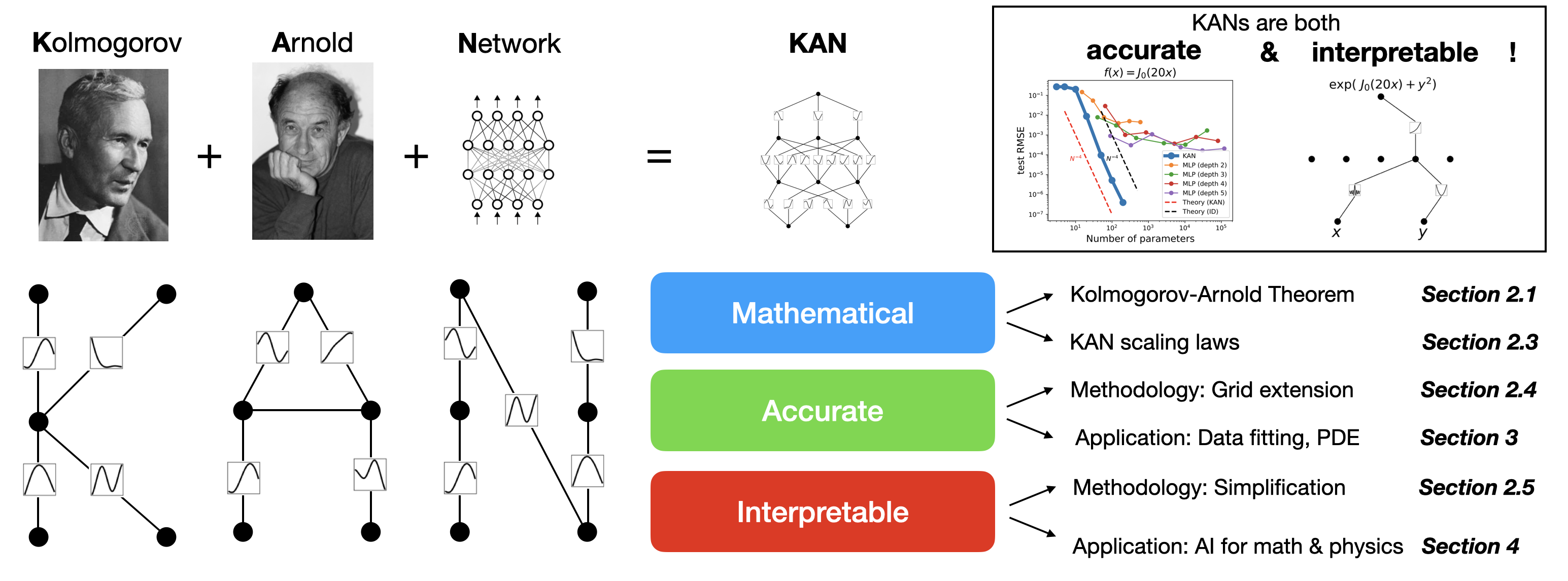
We propose a promising alternative to MLPs, called Kolmogorov-Arnold Networks (KANs). Whereas MLPs are inspired by the universal approximation theorem, KANs are inspired by the Kolmogorov-Arnold representation theorem [6, 7, 8]. Like MLPs, KANs have fully-connected structures. However, while MLPs place fixed activation functions on nodes ("neurons"), KANs place learnable activation functions on edges ("weights"), as illustrated in Figure 1. As a result, KANs have no linear weight matrices at all: instead, each weight parameter is replaced by a learnable 1D function parametrized as a spline. KANs' nodes simply sum incoming signals without applying any non-linearities. One might worry that KANs are hopelessly expensive, since each MLP's weight parameter becomes KAN's spline function. Fortunately, KANs usually allow much smaller computation graphs than MLPs.

Unsurprisingly, the possibility of using Kolmogorov-Arnold representation theorem to build neural networks has been studied [9, 10, 11, 12, 13, 14, 15, 16]. However, most work has stuck with the original depth-2 width-($2n+1$) representation, and many did not have the chance to leverage more modern techniques (e.g., back propagation) to train the networks. In [12], a depth-2 width-($2n+1$) representation was investigated, with breaking of the curse of dimensionality observed both empirically and with an approximation theory given compositional structures of the function. Our contribution lies in generalizing the original Kolmogorov-Arnold representation to arbitrary widths and depths, revitalizing and contextualizing it in today's deep learning world, as well as using extensive empirical experiments to highlight its potential for AI + Science due to its accuracy and interpretability.

Despite their elegant mathematical interpretation, KANs are nothing more than combinations of splines and MLPs, leveraging their respective strengths and avoiding their respective weaknesses. Splines are accurate for low-dimensional functions, easy to adjust locally, and able to switch between different resolutions. However, splines have a serious curse of dimensionality (COD) problem, because of their inability to exploit compositional structures. MLPs, on the other hand, suffer less from COD thanks to their feature learning, but are less accurate than splines in low dimensions, because of their inability to optimize univariate functions. The link between MLPs using ReLU-k as activation functions and splines have been established in [17, 18]. To learn a function accurately, a model should not only learn the compositional structure (external degrees of freedom), but should also approximate well the univariate functions (internal degrees of freedom). KANs are such models since they have MLPs on the outside and splines on the inside. As a result, KANs can not only learn features (thanks to their external similarity to MLPs), but can also optimize these learned features to great accuracy (thanks to their internal similarity to splines). For example, given a high dimensional function

$ \begin{align} f(x_1, \cdots, x_N)=\exp\left(\frac{1}{N}\sum_{i=1}^N {\rm sin}^2 (x_i)\right), \end{align} $

splines would fail for large $N$ due to COD; MLPs can potentially learn the the generalized additive structure, but they are very inefficient for approximating the exponential and sine functions with say, ReLU activations. In contrast, KANs can learn both the compositional structure and the univariate functions quite well, hence outperforming MLPs by a large margin (see Figure 6).

Throughout this paper, we will use extensive numerical experiments to show that KANs can lead to accuracy and interpretability improvement over MLPs, at least on small-scale AI + Science tasks. The organization of the paper is illustrated in Figure 2. In Section 2, we introduce the KAN architecture and its mathematical foundation, introduce network simplification techniques to make KANs interpretable, and introduce a grid extension technique to make KANs more accurate. In Section 3, we show that KANs are more accurate than MLPs for data fitting: KANs can beat the curse of dimensionality when there is a compositional structure in data, achieving better scaling laws than MLPs. We also demonstrate the potential of KANs in PDE solving via a simple example of the Poisson equation. In Section 4, we show that KANs are interpretable and can be used for scientific discoveries. We use two examples from mathematics (knot theory) and physics (Anderson localization) to demonstrate that KANs can be helpful "collaborators" for scientists to (re)discover math and physical laws. Section 5 summarizes related works. In Section 6, we conclude by discussing broad impacts and future directions. Codes are available at https://github.com/KindXiaoming/pykan and can also be installed via pip install pykan.

2. Kolmogorov–Arnold Networks (KAN)

Section Summary: Kolmogorov-Arnold Networks, or KANs, are a new kind of neural network inspired by a mathematical theorem from Andrey Kolmogorov and Vladimir Arnold, which shows that any complex, multi-variable continuous function can be broken down into simpler sums and compositions of single-variable functions. Unlike traditional multi-layer perceptrons that place activation functions on nodes, KANs put learnable one-dimensional functions, like smooth B-spline curves, directly on the connections between nodes, starting from the theorem's basic two-layer structure and extending it to deeper and wider networks for better performance. This design not only promises strong theoretical guarantees for accuracy but also allows techniques to refine precision through grid adjustments and simplify the network for easier human interpretation, making it potentially more useful for real-world machine learning tasks involving smooth, structured data.

Multi-Layer Perceptrons (MLPs) are inspired by the universal approximation theorem. We instead focus on the Kolmogorov-Arnold representation theorem, which can be realized by a new type of neural network called Kolmogorov-Arnold networks (KAN). We review the Kolmogorov-Arnold theorem in Section 2.1, to inspire the design of Kolmogorov-Arnold Networks in Section 2.2. In Section 2.3, we provide theoretical guarantees for the expressive power of KANs and their neural scaling laws, relating them to existing approximation and generalization theories in the literature. In Section 2.4, we propose a grid extension technique to make KANs increasingly more accurate. In Section 2.5, we propose simplification techniques to make KANs interpretable.

2.1 Kolmogorov-Arnold Representation theorem

Vladimir Arnold and Andrey Kolmogorov established that if $f$ is a multivariate continuous function on a bounded domain, then $f$ can be written as a finite composition of continuous functions of a single variable and the binary operation of addition. More specifically, for a smooth $f:[0, 1]^n\to\mathbb{R}$,

$ f(\mathbf{x}) = f(x_1, \cdots, x_n)=\sum_{q=1}^{2n+1} \Phi_q\left(\sum_{p=1}^n\phi_{q, p}(x_p)\right),\tag{1} $

where $\phi_{q, p}:[0, 1]\to\mathbb{R}$ and $\Phi_q:\mathbb{R}\to\mathbb{R}$. In a sense, they showed that the only true multivariate function is addition, since every other function can be written using univariate functions and sum. One might naively consider this great news for machine learning: learning a high-dimensional function boils down to learning a polynomial number of 1D functions. However, these 1D functions can be non-smooth and even fractal, so they may not be learnable in practice [19, 20]. Because of this pathological behavior, the Kolmogorov-Arnold representation theorem was basically sentenced to death in machine learning, regarded as theoretically sound but practically useless [19, 20].

However, we are more optimistic about the usefulness of the Kolmogorov-Arnold theorem for machine learning. First of all, we need not stick to the original Eq. (1) which has only two-layer non-linearities and a small number of terms ($2n+1$) in the hidden layer: we will generalize the network to arbitrary widths and depths. Secondly, most functions in science and daily life are often smooth and have sparse compositional structures, potentially facilitating smooth Kolmogorov-Arnold representations. The philosophy here is close to the mindset of physicists, who often care more about typical cases rather than worst cases. After all, our physical world and machine learning tasks must have structures to make physics and machine learning useful or generalizable at all [21].

2.2 KAN architecture

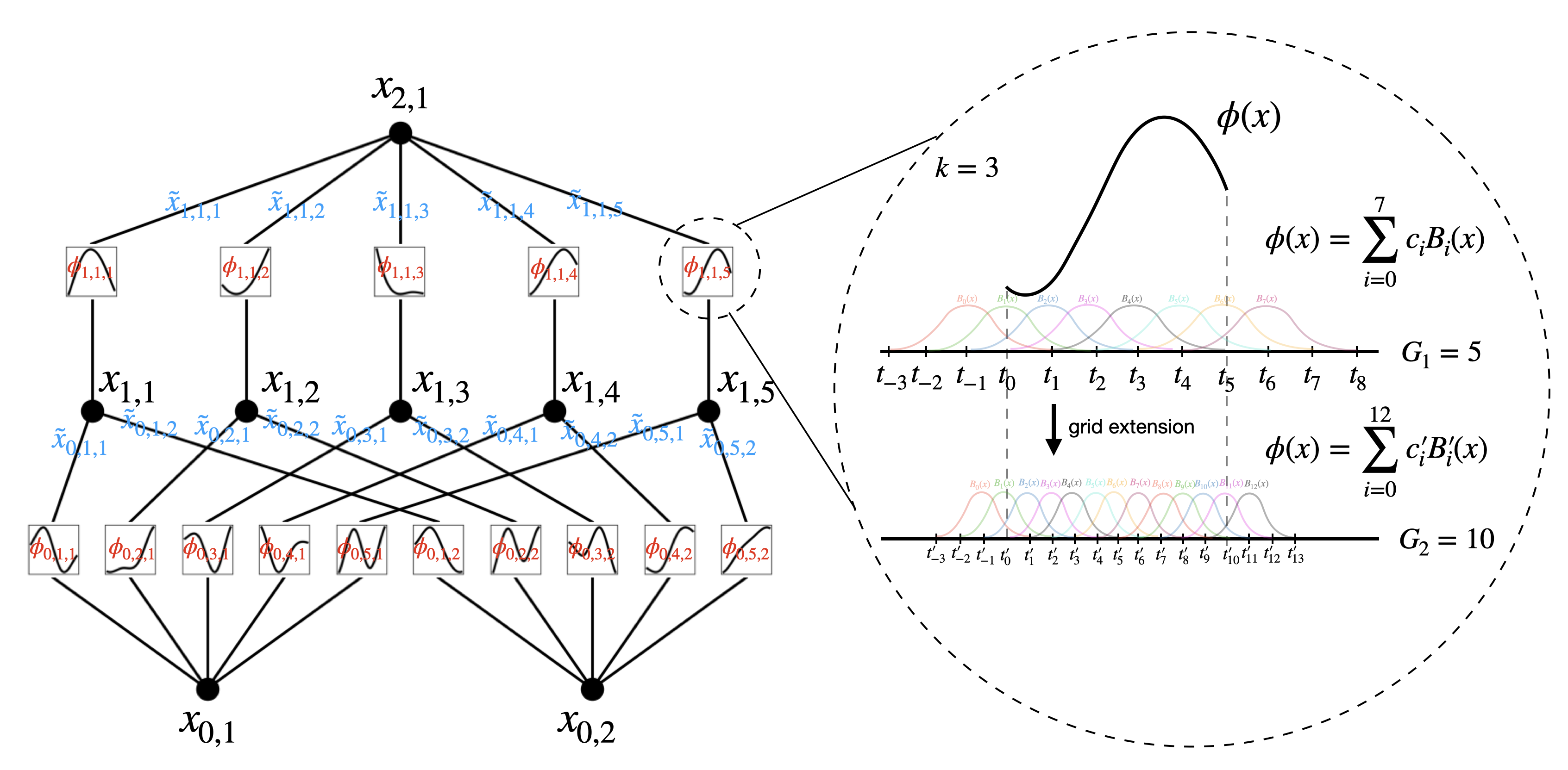
Suppose we have a supervised learning task consisting of input-output pairs ${\mathbf{x}_i, y_i}$, where we want to find $f$ such that $y_i\approx f(\mathbf{x}i)$ for all data points. Eq. (1) implies that we are done if we can find appropriate univariate functions $\phi{q, p}$ and $\Phi_q$. This inspires us to design a neural network which explicitly parametrizes Eq. (1). Since all functions to be learned are univariate functions, we can parametrize each 1D function as a B-spline curve, with learnable coefficients of local B-spline basis functions (see Figure 3 right). Now we have a prototype of KAN, whose computation graph is exactly specified by Eq. (1) and illustrated in Figure 1 (b) (with the input dimension $n=2$), appearing as a two-layer neural network with activation functions placed on edges instead of nodes (simple summation is performed on nodes), and with width $2n+1$ in the middle layer.

As mentioned, such a network is known to be too simple to approximate any function arbitrarily well in practice with smooth splines! We therefore generalize our KAN to be wider and deeper. It is not immediately clear how to make KANs deeper, since Kolmogorov-Arnold representations correspond to two-layer KANs. To the best of our knowledge, there is not yet a "generalized" version of the theorem that corresponds to deeper KANs.

The breakthrough occurs when we notice the analogy between MLPs and KANs. In MLPs, once we define a layer (which is composed of a linear transformation and nonlinearties), we can stack more layers to make the network deeper. To build deep KANs, we should first answer: "what is a KAN layer?" It turns out that a KAN layer with $n_{\rm in}$-dimensional inputs and $n_{\rm out}$-dimensional outputs can be defined as a matrix of 1D functions

$ \begin{align} {\mathbf\Phi}={\phi_{q, p}}, \qquad p=1, 2, \cdots, n_{\rm in}, \qquad q=1, 2\cdots, n_{\rm out}, \end{align} $

where the functions $\phi_{q, p}$ have trainable parameters, as detaild below. In the Kolmogov-Arnold theorem, the inner functions form a KAN layer with $n_{\rm in}=n$ and $n_{\rm out}=2n+1$, and the outer functions form a KAN layer with $n_{\rm in}=2n+1$ and $n_{\rm out}=1$. So the Kolmogorov-Arnold representations in Eq. (1) are simply compositions of two KAN layers. Now it becomes clear what it means to have deeper Kolmogorov-Arnold representations: simply stack more KAN layers!

Let us introduce some notation. This paragraph will be a bit technical, but readers can refer to Figure 3 (left) for a concrete example and intuitive understanding. The shape of a KAN is represented by an integer array

$ \begin{align} [n_0, n_1, \cdots, n_L], \end{align} $

where $n_i$ is the number of nodes in the $i^{\rm th}$ layer of the computational graph. We denote the $i^{\rm th}$ neuron in the $l^{\rm th}$ layer by $(l, i)$, and the activation value of the $(l, i)$-neuron by $x_{l, i}$. Between layer $l$ and layer $l+1$, there are $n_ln_{l+1}$ activation functions: the activation function that connects $(l, i)$ and $(l+1, j)$ is denoted by

$ \begin{align} \phi_{l, j, i}, \quad l=0, \cdots, L-1, \quad i=1, \cdots, n_{l}, \quad j=1, \cdots, n_{l+1}. \end{align} $

The pre-activation of $\phi_{l, j, i}$ is simply $x_{l, i}$; the post-activation of $\phi_{l, j, i}$ is denoted by $\tilde{x}{l, j, i}\equiv \phi{l, j, i}(x_{l, i})$. The activation value of the $(l+1, j)$ neuron is simply the sum of all incoming post-activations:

$ x_{l+1, j} = \sum_{i=1}^{n_l} \tilde{x}{l, j, i} = \sum{i=1}^{n_l}\phi_{l, j, i}(x_{l, i}), \qquad j=1, \cdots, n_{l+1}.\tag{2} $

In matrix form, this reads

$ \mathbf{x}{l+1} = \underbrace{\begin{pmatrix} \phi{l, 1, 1}(\cdot) & \phi_{l, 1, 2}(\cdot) & \cdots & \phi_{l, 1, n_{l}}(\cdot) \ \phi_{l, 2, 1}(\cdot) & \phi_{l, 2, 2}(\cdot) & \cdots & \phi_{l, 2, n_{l}}(\cdot) \ \vdots & \vdots & & \vdots \ \phi_{l, n_{l+1}, 1}(\cdot) & \phi_{l, n_{l+1}, 2}(\cdot) & \cdots & \phi_{l, n_{l+1}, n_{l}}(\cdot) \ \end{pmatrix}}_{\mathbf{\Phi}l} \mathbf{x}{l},\tag{3} $

where ${\mathbf \Phi}_l$ is the function matrix corresponding to the $l^{\rm th}$ KAN layer. A general KAN network is a composition of $L$ layers: given an input vector $\mathbf{x}_0\in\mathbb{R}^{n_0}$, the output of KAN is

$ {\rm KAN}(\mathbf{x}) = (\mathbf{\Phi}{L-1}\circ \mathbf{\Phi}{L-2}\circ\cdots\circ\mathbf{\Phi}{1}\circ\mathbf{\Phi}{0})\mathbf{x}.\tag{4} $

We can also rewrite the above equation to make it more analogous to Eq. (1), assuming output dimension $n_{L}=1$, and define $f(\mathbf{x})\equiv {\rm KAN}(\mathbf{x})$:

$ f(\mathbf{x})=\sum_{i_{L-1}=1}^{n_{L-1}}\phi_{L-1, i_{L}, i_{L-1}}\left(\sum_{i_{L-2}=1}^{n_{L-2}}\cdots\left(\sum_{i_2=1}^{n_2}\phi_{2, i_3, i_2}\left(\sum_{i_1=1}^{n_1}\phi_{1, i_2, i_1}\left(\sum_{i_0=1}^{n_0}\phi_{0, i_1, i_0}(x_{i_0})\right)\right)\right)\cdots\right), $

which is quite cumbersome. In contrast, our abstraction of KAN layers and their visualizations are cleaner and intuitive. The original Kolmogorov-Arnold representation Eq. (1) corresponds to a 2-Layer KAN with shape $[n, 2n+1, 1]$. Notice that all the operations are differentiable, so we can train KANs with back propagation. For comparison, an MLP can be written as interleaving of affine transformations $\mathbf{W}$ and non-linearities $\sigma$:

$ {\rm MLP}(\mathbf{x}) = (\mathbf{W}{L-1}\circ\sigma\circ \mathbf{W}{L-2}\circ\sigma\circ\cdots\circ\mathbf{W}_1\circ\sigma\circ\mathbf{W}_0)\mathbf{x}. $

It is clear that MLPs treat linear transformations and nonlinearities separately as $\mathbf{W}$ and $\sigma$, while KANs treat them all together in $\mathbf{\Phi}$. In Figure 1 (c) and (d), we visualize a three-layer MLP and a three-layer KAN, to clarify their differences.

Implementation details. Although a KAN layer Eq. (2) looks extremely simple, it is non-trivial to make it well optimizable. The key tricks are:

• (1) Residual activation functions. We include a basis function $b(x)$ (similar to residual connections) such that the activation function $\phi(x)$ is the sum of the basis function $b(x)$ and the spline function:

$ \begin{align} \phi(x)=w_{b} b(x)+w_{s}{\rm spline}(x). \end{align} $

We set

$ \begin{align} b(x)={\rm silu}(x)=x/(1+e^{-x}) \end{align} $

in most cases. ${\rm spline}(x)$ is parametrized as a linear combination of B-splines such that

$ \begin{align} {\rm spline}(x) = \sum_i c_iB_i(x) \end{align} $

where $c_i$ s are trainable (see Figure 3 for an illustration). In principle $w_b$ and $w_s$ are redundant since it can be absorbed into $b(x)$ and ${\rm spline}(x)$. However, we still include these factors (which are by default trainable) to better control the overall magnitude of the activation function.

• (2) Initialization scales. Each activation function is initialized to have $w_s=1$ and ${\rm spline}(x)\approx 0$ [^1]. $w_b$ is initialized according to the Xavier initialization, which has been used to initialize linear layers in MLPs.
• (3) Update of spline grids. We update each grid on the fly according to its input activations, to address the issue that splines are defined on bounded regions but activation values can evolve out of the fixed region during training [^2].

[^1]: This is done by drawing B-spline coefficients $c_i\sim\mathcal{N}(0,\sigma^2)$ with a small $\sigma$, typically we set $\sigma=0.1$.

[^2]: Other possibilities are: (a) the grid is learnable with gradient descent, e.g., [22]; (b) use normalization such that the input range is fixed. We tried (b) at first but its performance is inferior to our current approach.

Parameter count. For simplicity, let us assume a network

• (1) of depth $L$,
• (2) with layers of equal width $n_0=n_1=\cdots=n_{L}=N$,
• (3) with each spline of order $k$ (usually $k=3$) on $G$ intervals (for $G+1$ grid points).

Then there are in total $O(N^2L(G+k))\sim O(N^2LG)$ parameters. In contrast, an MLP with depth $L$ and width $N$ only needs $O(N^2L)$ parameters, which appears to be more efficient than KAN. Fortunately, KANs usually require much smaller $N$ than MLPs, which not only saves parameters, but also achieves better generalization (see e.g., Figure 6 and Figure 8) and facilitates interpretability. We remark that for 1D problems, we can take $N=L=1$ and the KAN network in our implementation is nothing but a spline approximation. For higher dimensions, we characterize the generalization behavior of KANs with a theorem below.

2.3 KAN's Approximation Abilities and Scaling Laws

Recall that in Equation 1, the 2-Layer width- $(2n+1)$ representation may be non-smooth. However, deeper representations may bring the advantages of smoother activations. For example, the 4-variable function

$ \begin{align} f(x_1, x_2, x_3, x_4)=\exp\left({\sin}(x_1^2+x_2^2)+{\sin}(x_3^2+x_4^2)\right) \end{align} $

can be smoothly represented by a $[4, 2, 1, 1]$ KAN which is 3-Layer, but may not admit a 2-Layer KAN with smooth activations. To facilitate an approximation analysis, we still assume smoothness of activations, but allow the representations to be arbitrarily wide and deep, as in Eq. (4). To emphasize the dependence of our KAN on the finite set of grid points, we use $\mathbf{\Phi}l^G$ and $\Phi{l, i, j}^G$ below to replace the notation $\mathbf{\Phi}l$ and $\Phi{l, i, j}$ used in Equation 2 and 3.

########## {caption="Theorem 1: Approximation theory, KAT"}

Let $\mathbf{x}=(x_1, x_2, \cdots, x_n)$. Suppose that a function $f(\mathbf{x})$ admits a representation

$ f = (\mathbf{\Phi}{L-1}\circ\mathbf{\Phi}{L-2}\circ\cdots\circ\mathbf{\Phi}{1}\circ\mathbf{\Phi}{0})\mathbf{x}, , $

as in Equation 4, where each one of the $\Phi_{l, i, j}$ are $(k+1)$-times continuously differentiable. Then there exists a constant $C$ depending on $f$ and its representation, such that we have the following approximation bound in terms of the grid size $G$: there exist $k$-th order B-spline functions $\Phi_{l, i, j}^G$ such that for any $0\leq m\leq k$, we have the bound

$ |f-(\mathbf{\Phi}^G_{L-1}\circ\mathbf{\Phi}^G_{L-2}\circ\cdots\circ\mathbf{\Phi}^G_{1}\circ\mathbf{\Phi}^G_{0})\mathbf{x}|_{C^m}\leq CG^{-k-1+m}, .\tag{5} $

Here we adopt the notation of $C^m$-norm measuring the magnitude of derivatives up to order $m$:

$ |g|_{C^m}=\max _{|\beta| \leq m} \sup _{x\in [0, 1]^n}\left|D^\beta g(x)\right| . $

Proof: By the classical 1D B-spline theory [23] and the fact that $\Phi_{l, i, j}$ as continuous functions can be uniformly bounded on a bounded domain, we know that there exist finite-grid B-spline functions $\Phi_{l, i, j}^G$ such that for any 0 $\leq m\leq k$,

$ |(\Phi_{l, i, j}\circ\mathbf{\Phi}{l-1}\circ\mathbf{\Phi}{l-2}\circ\cdots\circ\mathbf{\Phi}{1}\circ\mathbf{\Phi}{0})\mathbf{x}-(\Phi_{l, i, j}^G\circ\mathbf{\Phi}{l-1}\circ\mathbf{\Phi}{l-2}\circ\cdots\circ\mathbf{\Phi}{1}\circ\mathbf{\Phi}{0})\mathbf{x}|_{C^m}\leq CG^{-k-1+m}, , $

with a constant $C$ independent of $G$. We fix those B-spline approximations. Therefore we have that the residue $R_l$ defined via

$ R_l\coloneqq (\mathbf{\Phi}^G_{L-1}\circ\cdots\circ\mathbf{\Phi}^G_{l+1}\circ\mathbf{\Phi}{l}\circ\mathbf{\Phi}{l-1}\circ\cdots\circ\mathbf{\Phi}{0})\mathbf{x}-(\mathbf{\Phi}{L-1}^G\circ\cdots\circ\mathbf{\Phi}{l+1}^G\circ\mathbf{\Phi}{l}^G\circ\mathbf{\Phi}{l-1}\circ\cdots\circ\mathbf{\Phi}{0})\mathbf{x} $

satisfies

$ |R_l|_{C^m}\leq CG^{-k-1+m}, , $

with a constant independent of $G$. Finally notice that

$ f-(\mathbf{\Phi}^G_{L-1}\circ\mathbf{\Phi}^G_{L-2}\circ\cdots\circ\mathbf{\Phi}^G_{1}\circ\mathbf{\Phi}^G_{0})\mathbf{x}=R_{L-1}+R_{L-2}+\cdots+R_1+R_0, , $

we know that Equation 5 holds.

We know that asymptotically, provided that the assumption in Theorem 1 holds, KANs with finite grid size can approximate the function well with a residue rate independent of the dimension, hence beating curse of dimensionality! This comes naturally since we only use splines to approximate 1D functions. In particular, for $m=0$, we recover the accuracy in $L^\infty$ norm, which in turn provides a bound of RMSE on the finite domain, which gives a scaling exponent $k+1$. Of course, the constant $C$ is dependent on the representation; hence it will depend on the dimension. We will leave the discussion of the dependence of the constant on the dimension as a future work.

We remark that although the Kolmogorov-Arnold theorem Eq. (1) corresponds to a KAN representation with shape $[d, 2d+1, 1]$, its functions are not necessarily smooth. On the other hand, if we are able to identify a smooth representation (maybe at the cost of extra layers or making the KAN wider than the theory prescribes), then Theorem 1 indicates that we can beat the curse of dimensionality (COD). This should not come as a surprise since we can inherently learn the structure of the function and make our finite-sample KAN approximation interpretable.

Neural scaling laws: comparison to other theories. Neural scaling laws are the phenomenon where test loss decreases with more model parameters, i.e., $\ell\propto N^{-\alpha}$ where $\ell$ is test RMSE, $N$ is the number of parameters, and $\alpha$ is the scaling exponent. A larger $\alpha$ promises more improvement by simply scaling up the model. Different theories have been proposed to predict $\alpha$. Sharma & Kaplan [24] suggest that $\alpha$ comes from data fitting on an input manifold of intrinsic dimensionality $d$. If the model function class is piecewise polynomials of order $k$ ($k=1$ for ReLU), then the standard approximation theory implies $\alpha=(k+1)/d$ from the approximation theory. This bound suffers from the curse of dimensionality, so people have sought other bounds independent of $d$ by leveraging compositional structures. In particular, Michaud et al. [25] considered computational graphs that only involve unary (e.g., squared, sine, exp) and binary ($+$ and $\times$) operations, finding $\alpha=(k+1)/d^*=(k+1)/2$, where $d^*=2$ is the maximum arity. Poggio et al. [19] leveraged the idea of compositional sparsity and proved that given function class $W_m$ (function whose derivatives are continuous up to $m$-th order), one needs $N=O(\epsilon^{-\frac{2}{m}})$ number of parameters to achieve error $\epsilon$, which is equivalent to $\alpha=\frac{m}{2}$. Our approach, which assumes the existence of smooth Kolmogorov-Arnold representations, decomposes the high-dimensional function into several 1D functions, giving $\alpha=k+1$ (where $k$ is the piecewise polynomial order of the splines). We choose $k=3$ cubic splines so $\alpha=4$ which is the largest and best scaling exponent compared to other works. We will show in Section 3.1 that this bound $\alpha=4$ can in fact be achieved empirically with KANs, while previous work [25] reported that MLPs have problems even saturating slower bounds (e.g., $\alpha=1$) and plateau quickly. Of course, we can increase $k$ to match the smoothness of functions, but too high $k$ might be too oscillatory, leading to optimization issues.

Comparison between KAT and UAT. The power of fully-connected neural networks is justified by the universal approximation theorem (UAT), which states that given a function and error tolerance $\epsilon>0$, a two-layer network with $k>N(\epsilon)$ neurons can approximate the function within error $\epsilon$. However, the UAT guarantees no bound for how $N(\epsilon)$ scales with $\epsilon$. Indeed, it suffers from the COD, and $N$ has been shown to grow exponentially with $d$ in some cases [21]. The difference between KAT and UAT is a consequence that KANs take advantage of the intrinsically low-dimensional representation of the function while MLPs do not. In KAT, we highlight quantifying the approximation error in the compositional space. In the literature, generalization error bounds, taking into account finite samples of training data, for a similar space have been studied for regression problems; see [26, 27], and also specifically for MLPs with ReLU activations [28]. On the other hand, for general function spaces like Sobolev or Besov spaces, the nonlinear $n$-widths theory [29, 30, 31] indicates that we can never beat the curse of dimensionality, while MLPs with ReLU activations can achieve the tight rate [32, 33, 34]. This fact again motivates us to consider functions of compositional structure, the much "nicer" functions that we encounter in practice and in science, to overcome the COD. Compared with MLPs, we may use a smaller architecture in practice, since we learn general nonlinear activation functions; see also [28] where the depth of the ReLU MLPs needs to reach at least $\log n$ to have the desired rate, where $n$ is the number of samples. Indeed, we will show that KANs are nicely aligned with symbolic functions while MLPs are not.

2.4 For accuracy: Grid Extension

In principle, a spline can be made arbitrarily accurate to a target function as the grid can be made arbitrarily fine-grained. This good feature is inherited by KANs. By contrast, MLPs do not have the notion of "fine-graining". Admittedly, increasing the width and depth of MLPs can lead to improvement in performance ("neural scaling laws"). However, these neural scaling laws are slow (discussed in the last section). They are also expensive to obtain, because models of varying sizes are trained independently. By contrast, for KANs, one can first train a KAN with fewer parameters and then extend it to a KAN with more parameters by simply making its spline grids finer, without the need to retraining the larger model from scratch.

We next describe how to perform grid extension (illustrated in Figure 3 right), which is basically fitting a new fine-grained spline to an old coarse-grained spline. Suppose we want to approximate a 1D function $f$ in a bounded region $[a, b]$ with B-splines of order $k$. A coarse-grained grid with $G_1$ intervals has grid points at ${t_0=a, t_1, t_2, \cdots, t_{G_1}=b}$, which is augmented to ${t_{-k}, \cdots, t_{-1}, t_0, \cdots, t_{G_1}, t_{G_1+1}, \cdots, t_{G_1+k}}$. There are $G_1+k$ B-spline basis functions, with the $i^{\rm th}$ B-spline $B_i(x)$ being non-zero only on $[t_{-k+i}, t_{i+1}]$ $(i=0, \cdots, G_1+k-1)$. Then $f$ on the coarse grid is expressed in terms of linear combination of these B-splines basis functions $f_{\rm coarse}(x)=\sum_{i=0}^{G_1+k-1} c_i B_i(x)$. Given a finer grid with $G_2$ intervals, $f$ on the fine grid is correspondingly $f_{\rm fine}(x)=\sum_{j=0}^{G_2+k-1}c_j'B_j'(x)$. The parameters $c'j$ s can be initialized from the parameters $c_i$ by minimizing the distance between $f{\rm fine}(x)$ to $f_{\rm coarse}(x)$ (over some distribution of $x$):

$ {c_j'} = \underset{{c_j'}}{\rm argmin}\ \mathop{\mathbb{E}}{x\sim p(x)}\left(\sum{j=0}^{G_2+k-1}c_j'B_j'(x)-\sum_{i=0}^{G_1+k-1} c_i B_i(x)\right)^2, $

which can be implemented by the least squares algorithm. We perform grid extension for all splines in a KAN independently.

Toy example: staricase-like loss curves. We use a toy example $f(x, y)={\rm exp}({\rm sin}(\pi x)+y^2)$ to demonstrate the effect of grid extension. In Figure 4 (top left), we show the train and test RMSE for a $[2, 5, 1]$ KAN. The number of grid points starts as 3, increases to a higher value every 200 LBFGS steps, ending up with 1000 grid points. It is clear that every time fine graining happens, the training loss drops faster than before (except for the finest grid with 1000 points, where optimization ceases to work probably due to bad loss landscapes). However, the test losses first go down then go up, displaying a U-shape, due to the bias-variance tradeoff (underfitting vs. overfitting). We conjecture that the optimal test loss is achieved at the interpolation threshold when the number of parameters match the number of data points. Since our training samples are 1000 and the total parameters of a $[2, 5, 1]$ KAN is $15G$ ($G$ is the number of grid intervals), we expect the interpolation threshold to be $G=1000/15\approx 67$, which roughly agrees with our experimentally observed value $G\sim 50$.

Small KANs generalize better. Is this the best test performance we can achieve? Notice that the synthetic task can be represented exactly by a $[2, 1, 1]$ KAN, so we train a $[2, 1, 1]$ KAN and present the training dynamics in Figure 4 top right. Interestingly, it can achieve even lower test losses than the $[2, 5, 1]$ KAN, with clearer staircase structures and the interpolation threshold is delayed to a larger grid size as a result of fewer parameters. This highlights a subtlety of choosing KAN architectures. If we do not know the problem structure, how can we determine the minimal KAN shape? In Section 2.5, we will propose a method to auto-discover such minimal KAN architecture via regularization and pruning.

Scaling laws: comparison with theory. We are also interested in how the test loss decreases as the number of grid parameters increases. In Figure 4 (bottom left), a [2, 1, 1] KAN scales roughly as ${\rm test \ RMSE}\propto G^{-3}$. However, according to the Theorem 1, we would expect ${\rm test \ RMSE}\propto G^{-4}$. We found that the errors across samples are not uniform. This is probably attributed to boundary effects [25]. In fact, there are a few samples that have significantly larger errors than others, making the overall scaling slow down. If we plot the square root of the median (not mean) of the squared losses, we get a scaling closer to $G^{-4}$. Despite this suboptimality (probably due to optimization), KANs still have much better scaling laws than MLPs, for data fitting (Figure 6) and PDE solving (Figure 8). In addition, the training time scales favorably with the number of grid points $G$, shown in Figure 4 bottom right [^3].

[^3]: When $G=1000$, training becomes significantly slower, which is specific to the use of the LBFGS optimizer with line search. We conjecture that the loss landscape becomes bad for $G=1000$, so line search with trying to find an optimal step size within maximal iterations without early stopping.

External vs Internal degrees of freedom. A new concept that KANs highlights is a distinction between external versus internal degrees of freedom (parameters). The computational graph of how nodes are connected represents external degrees of freedom ("dofs"), while the grid points inside an activation function are internal degrees of freedom. KANs benefit from the fact that they have both external dofs and internal dofs. External dofs (that MLPs also have but splines do not) are responsible for learning compositional structures of multiple variables. Internal dofs (that splines also have but MLPs do not) are responsible for learning univariate functions.

2.5 For Interpretability: Simplifying KANs and Making them interactive

One loose end from the last subsection is that we do not know how to choose the KAN shape that best matches the structure of a dataset. For example, if we know that the dataset is generated via the symbolic formula $f(x, y) = {\rm exp}({\rm sin}(\pi x)+y^2)$, then we know that a $[2, 1, 1]$ KAN is able to express this function. However, in practice we do not know the information a priori, so it would be nice to have approaches to determine this shape automatically. The idea is to start from a large enough KAN and train it with sparsity regularization followed by pruning. We will show that these pruned KANs are much more interpretable than non-pruned ones. To make KANs maximally interpretable, we propose a few simplification techniques in Section 2.5.1, and an example of how users can interact with KANs to make them more interpretable in Section 2.5.2.

2.5.1 Simplification techniques

1. Sparsification. For MLPs, L1 regularization of linear weights is used to favor sparsity. KANs can adapt this high-level idea, but need two modifications:

• (1) There is no linear "weight" in KANs. Linear weights are replaced by learnable activation functions, so we should define the L1 norm of these activation functions.
• (2) We find L1 to be insufficient for sparsification of KANs; instead an additional entropy regularization is necessary (see Appendix C for more details).

We define the L1 norm of an activation function $\phi$ to be its average magnitude over its $N_p$ inputs, i.e.,

$ \left|\phi\right|1 \equiv \frac{1}{N_p}\sum{s=1}^{N_p} \left|\phi(x^{(s)})\right|. $

Then for a KAN layer $\mathbf{\Phi}$ with $n_{\rm in}$ inputs and $n_{\rm out}$ outputs, we define the L1 norm of $\mathbf{\Phi}$ to be the sum of L1 norms of all activation functions, i.e.,

$ \left|\mathbf{\Phi}\right|1 \equiv \sum{i=1}^{n_{\rm in}}\sum_{j=1}^{n_{\rm out}} \left|\phi_{i, j}\right|_1. $

In addition, we define the entropy of $\mathbf{\Phi}$ to be

$ S(\mathbf{\Phi}) \equiv -\sum_{i=1}^{n_{\rm in}}\sum_{j=1}^{n_{\rm out}} \frac{\left|\phi_{i, j}\right|_1}{\left|\mathbf{\Phi}\right|1}{\rm log}\left(\frac{\left|\phi{i, j}\right|_1}{\left|\mathbf{\Phi}\right|_1}\right). $

The total training objective $\ell_{\rm total}$ is the prediction loss $\ell_{\rm pred}$ plus L1 and entropy regularization of all KAN layers:

$ \ell_{\rm total} = \ell_{\rm pred} + \lambda \left(\mu_1 \sum_{l=0}^{L-1}\left|\mathbf{\Phi}_l\right|1 + \mu_2 \sum{l=0}^{L-1}S(\mathbf{\Phi}_l)\right), $

where $\mu_1, \mu_2$ are relative magnitudes usually set to $\mu_1=\mu_2=1$, and $\lambda$ controls overall regularization magnitude.

2. Visualization. When we visualize a KAN, to get a sense of magnitudes, we set the transparency of an activation function $\phi_{l, i, j}$ proportional to ${\rm tanh}(\beta A_{l, i, j})$ where $\beta=3$ . Hence, functions with small magnitude appear faded out to allow us to focus on important ones.

3. Pruning. After training with sparsification penalty, we may also want to prune the network to a smaller subnetwork. We sparsify KANs on the node level (rather than on the edge level). For each node (say the $i^{\rm th}$ neuron in the $l^{\rm th}$ layer), we define its incoming and outgoing score as

$ I_{l, i} = \underset{k}{\rm max}(\left|\phi_{l-1, i, k}\right|1), \qquad O{l, i} = \underset{j}{\rm max}(\left|\phi_{l+1, j, i}\right|_1), $

and consider a node to be important if both incoming and outgoing scores are greater than a threshold hyperparameter $\theta=10^{-2}$ by default. All unimportant neurons are pruned.

4. Symbolification. In cases where we suspect that some activation functions are in fact symbolic (e.g., ${\rm cos}$ or ${\rm log}$), we provide an interface to set them to be a specified symbolic form, $\texttt{fix_symbolic(l, i, j, f)}$ can set the $(l, i, j)$ activation to be $f$. However, we cannot simply set the activation function to be the exact symbolic formula, since its inputs and outputs may have shifts and scalings. So, we obtain preactivations $x$ and postactivations $y$ from samples, and fit affine parameters $(a, b, c, d)$ such that $y\approx cf(ax+b)+d$. The fitting is done by iterative grid search of $a, b$ and linear regression.

Besides these techniques, we provide additional tools that allow users to apply more fine-grained control to KANs, listed in Appendix A.

2.5.2 A toy example: how humans can interact with KANs

Above we have proposed a number of simplification techniques for KANs. We can view these simplification choices as buttons one can click on. A user interacting with these buttons can decide which button is most promising to click next to make KANs more interpretable. We use an example below to showcase how a user could interact with a KAN to obtain maximally interpretable results.

Let us again consider the regression task

$ \begin{align} f(x, y) = \exp\left({\sin}(\pi x)+y^2\right). \end{align} $

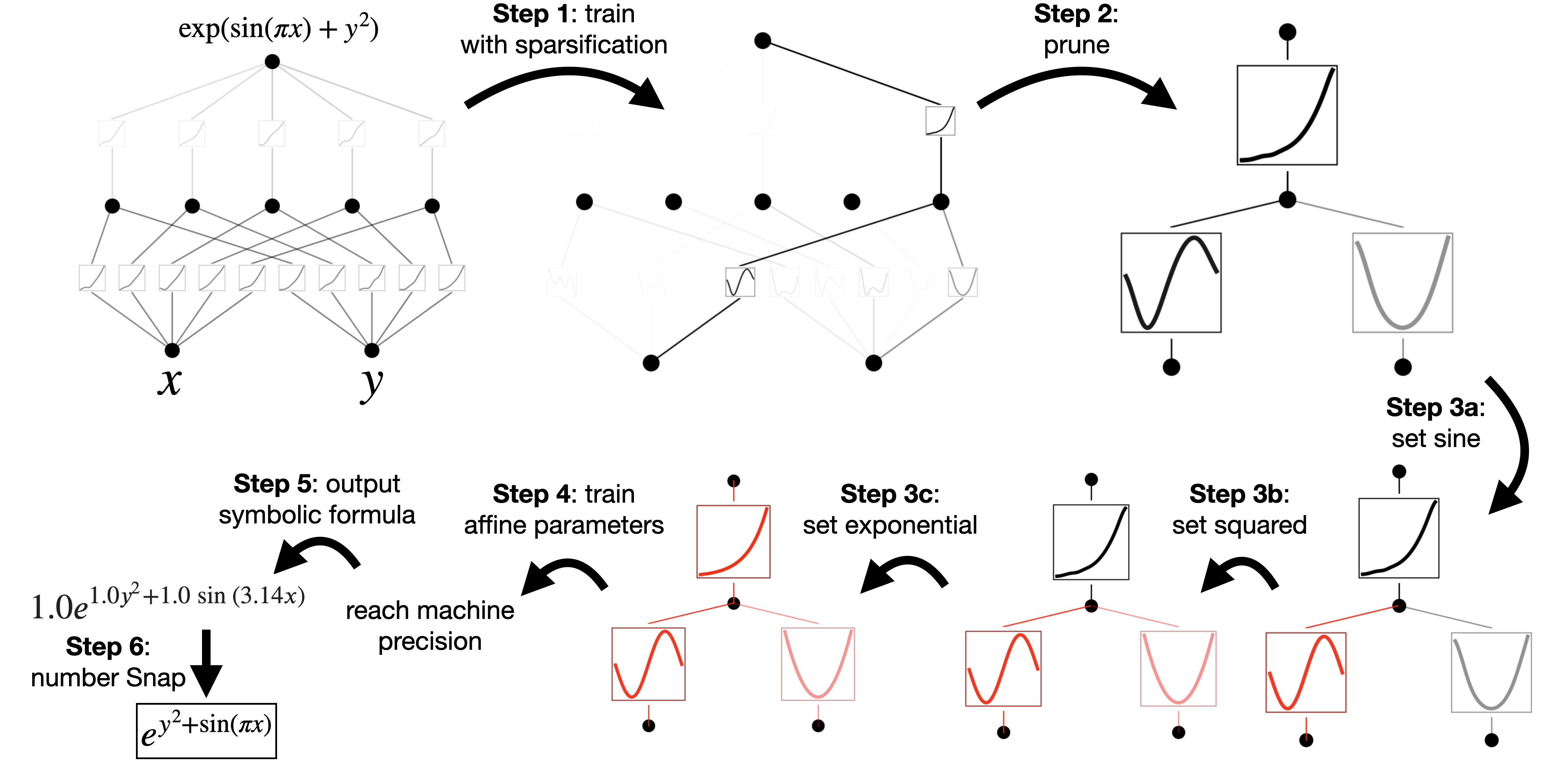
Given data points $(x_i, y_i, f_i)$, $i=1, 2, \cdots, N_p$, a hypothetical user Alice is interested in figuring out the symbolic formula. The steps of Alice's interaction with the KANs are described below (illustrated in Figure 5):

Step 1: Training with sparsification. Starting from a fully-connected $[2, 5, 1]$ KAN, training with sparsification regularization can make it quite sparse. 4 out of 5 neurons in the hidden layer appear useless, hence we want to prune them away.

Step 2: Pruning. Automatic pruning is seen to discard all hidden neurons except the last one, leaving a $[2, 1, 1]$ KAN. The activation functions appear to be known symbolic functions.

Step 3: Setting symbolic functions. Assuming that the user can correctly guess these symbolic formulas from staring at the KAN plot, they can set

$ \begin{aligned} &\texttt{fix_symbolic(0, 0, 0, sin')} \\ &\texttt{fix\_symbolic(0, 1, 0, x^2')} \ &\texttt{fix_symbolic(1, 0, 0, `exp')}. \end{aligned} $

In case the user has no domain knowledge or no idea which symbolic functions these activation functions might be, we provide a function $\texttt{suggest_symbolic}$ to suggest symbolic candidates.

Step 4: Further training. After symbolifying all the activation functions in the network, the only remaining parameters are the affine parameters. We continue training these affine parameters, and when we see the loss dropping to machine precision, we know that we have found the correct symbolic expression.

Step 5: Output the symbolic formula. Sympy is used to compute the symbolic formula of the output node. The user obtains $1.0e^{1.0y^2+1.0{\rm sin}(3.14x)}$, which is the true answer (we only displayed two decimals for $\pi$).

Remark: Why not symbolic regression (SR)? It is reasonable to use symbolic regression for this example. However, symbolic regression methods are in general brittle and hard to debug. They either return a success or a failure in the end without outputting interpretable intermediate results. In contrast, KANs do continuous search (with gradient descent) in function space, so their results are more continuous and hence more robust. Moreover, users have more control over KANs as compared to SR due to KANs' transparency. The way we visualize KANs is like displaying KANs' "brain" to users, and users can perform "surgery" (debugging) on KANs. This level of control is typically unavailable for SR. We will show examples of this in Section 4.4. More generally, when the target function is not symbolic, symbolic regression will fail but KANs can still provide something meaningful. For example, a special function (e.g., a Bessel function) is impossible to SR to learn unless it is provided in advance, but KANs can use splines to approximate it numerically anyway (see Figure 10 (d)).

3. KANs are accurate

Section Summary: This section explains how Kolmogorov-Arnold Networks (KANs) outperform multilayer perceptrons (MLPs) in accurately representing various functions, such as in regression tasks and solving partial differential equations, by achieving lower errors with fewer parameters. On toy datasets with known simple structures, KANs scale efficiently toward theoretical performance limits, closely fitting complex curves like Bessel functions or exponentials, while MLPs converge slowly and hit plateaus. For special mathematical functions, like those used in physics, KANs even discover compact representations without prior knowledge, consistently showing superior accuracy and efficiency compared to MLPs across multiple examples.

In this section, we demonstrate that KANs are more effective at representing functions than MLPs in various tasks (regression and PDE solving). When comparing two families of models, it is fair to compare both their accuracy (loss) and their complexity (number of parameters). We will show that KANs display more favorable Pareto Frontiers than MLPs. Moreover, in Section 3.5, we show that KANs can naturally work in continual learning without catastrophic forgetting.

3.1 Toy datasets

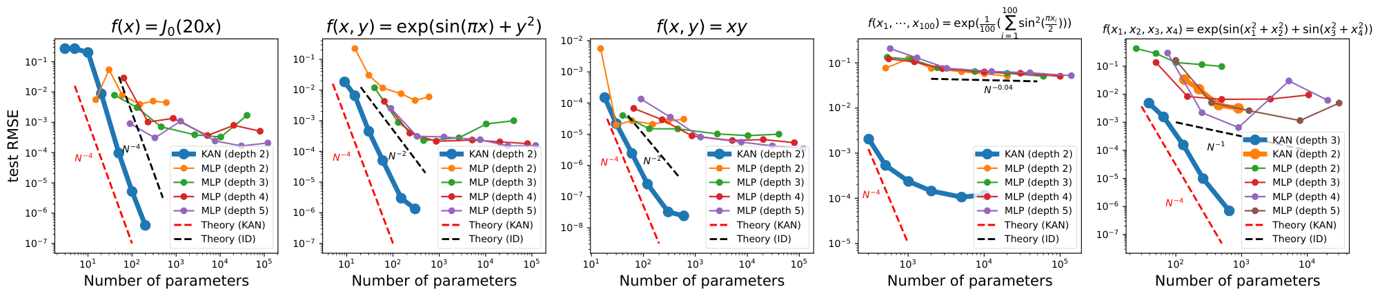
In Section 2.3, our theory suggested that test RMSE loss $\ell$ scales as $\ell\propto N^{-4}$ with model parameters $N$. However, this relies on the existence of a Kolmogorov-Arnold representation. As a sanity check, we construct five examples we know have smooth KA representations:

• (1) $f(x)=J_0(20x)$, which is the Bessel function. Since it is a univariate function, it can be represented by a spline, which is a $[1, 1]$ KAN.
• (2) $f(x, y)={\rm exp}({\rm sin}(\pi x)+y^2)$. We know that it can be exactly represented by a $[2, 1, 1]$ KAN.
• (3) $f(x, y)=xy$. We know from Figure 10 that it can be exactly represented by a $[2, 2, 1]$ KAN.
• (4) A high-dimensional example $f(x_1, \cdots, x_{100})={\rm exp}(\frac{1}{100}\sum_{i=1}^{100}{\rm sin}^2(\frac{\pi x_i}{2}))$ which can be represented by a $[100, 1, 1]$ KAN.
• (5) A four-dimensional example $f(x_1, x_2, x_3, x_4)={\rm exp}(\frac{1}{2}({\rm sin}(\pi(x_1^2+x_2^2))+{\rm sin}(\pi(x_3^2+x_4^2))))$ which can be represented by a $[4, 4, 2, 1]$ KAN.

We train these KANs by increasing grid points every 200 steps, in total covering $G={3, 5, 10, 20, 50, 100, 200, 500, 1000}$. We train MLPs with different depths and widths as baselines. Both MLPs and KANs are trained with LBFGS for 1800 steps in total. We plot test RMSE as a function of the number of parameters for KANs and MLPs in Figure 6, showing that KANs have better scaling curves than MLPs, especially for the high-dimensional example. For comparison, we plot the lines predicted from our KAN theory as red dashed ($\alpha=k+1=4$), and the lines predicted from Sharma & Kaplan [24] as black-dashed ($\alpha=(k+1)/d=4/d$). KANs can almost saturate the steeper red lines, while MLPs struggle to converge even as fast as the slower black lines and plateau quickly. We also note that for the last example, the 2-Layer KAN $[4, 9, 1]$ behaves much worse than the 3-Layer KAN (shape $[4, 2, 2, 1]$). This highlights the greater expressive power of deeper KANs, which is the same for MLPs: deeper MLPs have more expressive power than shallower ones. Note that we have adopted the vanilla setup where both KANs and MLPs are trained with LBFGS without advanced techniques, e.g., switching between Adam and LBFGS, or boosting [35]. We leave the comparison of KANs and MLPs in advanced setups for future work.

3.2 Special functions

One caveat for the above results is that we assume knowledge of the "true" KAN shape. In practice, we do not know the existence of KA representations. Even when we are promised that such a KA representation exists, we do not know the KAN shape a priori. Special functions in more than one variables are such cases, because it would be (mathematically) surprising if multivariate special functions (e.g., a Bessel function $f(\nu, x)=J_\nu(x)$) could be written in KA represenations, involving only univariate functions and sums). We show below that:

• (1) Finding (approximate) compact KA representations of special functions is possible, revealing novel mathematical properties of special functions from the perspective of Kolmogorov-Arnold representations.
• (2) KANs are more efficient and accurate in representing special functions than MLPs.

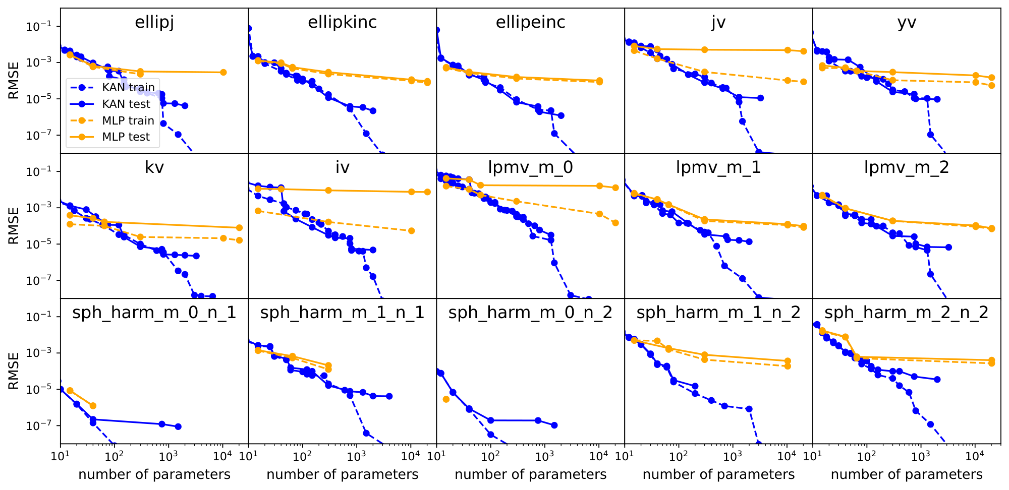
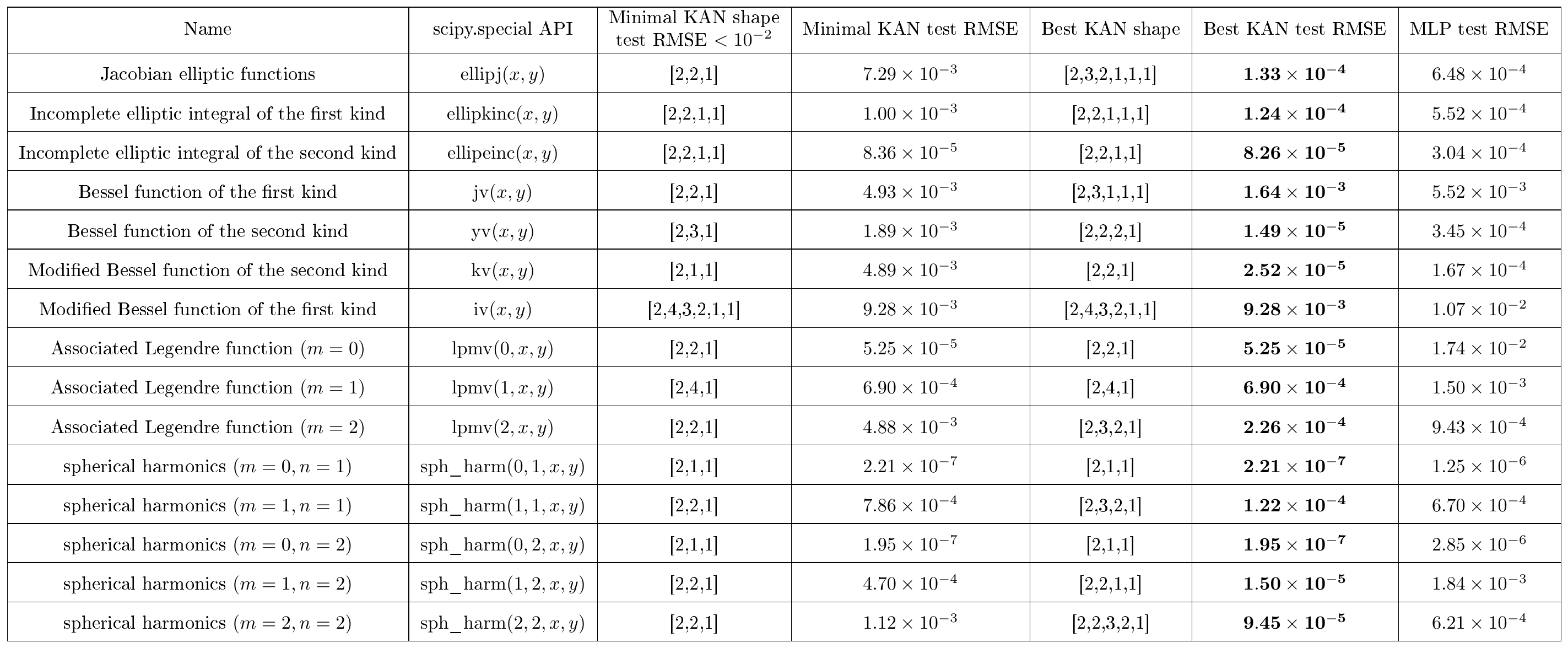
We collect 15 special functions common in math and physics, summarized in Table 1. We choose MLPs with fixed width 5 or 100 and depths swept in ${2, 3, 4, 5, 6}$. We run KANs both with and without pruning. KANs without pruning: We fix the shape of KAN, whose width are set to 5 and depths are swept in 2, 3, 4, 5, 6. KAN with pruning. We use the sparsification $(\lambda=10^{-2}\ {\rm or}\ 10^{-3})$ and pruning technique in Section 2.5.1 to obtain a smaller KAN pruned from a fixed-shape KAN. Each KAN is initialized to have $G=3$, trained with LBFGS, with increasing number of grid points every 200 steps to cover $G={3, 5, 10, 20, 50, 100, 200}$. For each hyperparameter combination, we run 3 random seeds.

For each dataset and each model family (KANs or MLPs), we plot the Pareto frontier [^4], in the (number of parameters, RMSE) plane, shown in Figure 7. KANs' performance is shown to be consistently better than MLPs, i.e., KANs can achieve lower training/test losses than MLPs, given the same number of parameters. Moreover, we report the (surprisingly compact) shapes of our auto-discovered KANs for special functions in Table 1. On one hand, it is interesting to interpret what these compact representations mean mathematically (we include the KAN illustrations in Figure 24 and Figure 25 in Appendix F). On the other hand, these compact representations imply the possibility of breaking down a high-dimensional lookup table into several 1D lookup tables, which can potentially save a lot of memory, with the (almost negligible) overhead to perform a few additions at inference time.

[^4]: Pareto frontier is defined as fits that are optimal in the sense of no other fit being both simpler and more accurate.

::: {caption="Table 1: Special functions"}

:::

3.3 Feynman datasets

The setup in Section 3.1 is when we clearly know "true" KAN shapes. The setup in Section 3.2 is when we clearly do not know "true" KAN shapes. This part investigates a setup lying in the middle: Given the structure of the dataset, we may construct KANs by hand, but we are not sure if they are optimal. In this regime, it is interesting to compare human-constructed KANs and auto-discovered KANs via pruning (techniques in Section 2.5.1).

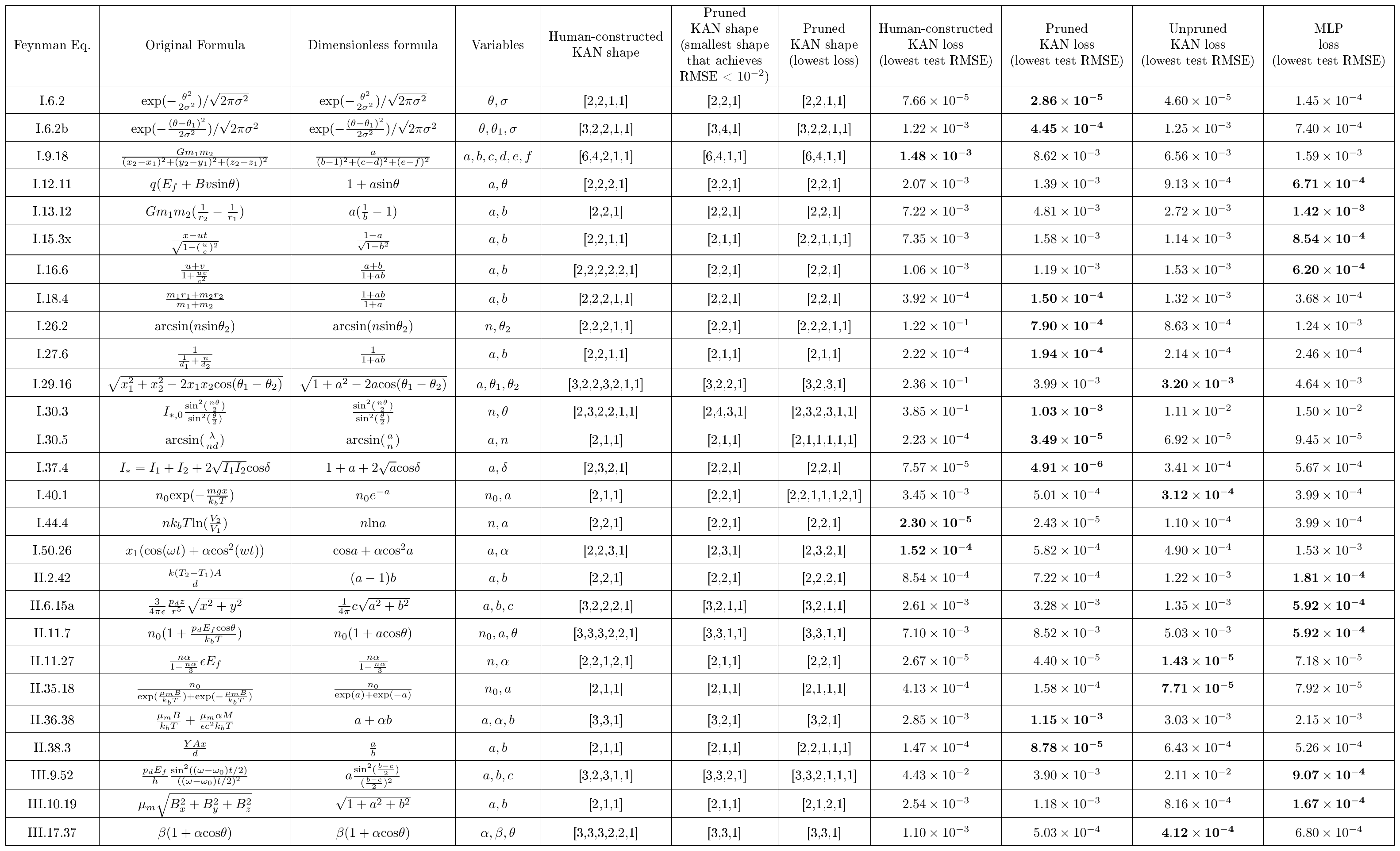
::: {caption="Table 2: Feynman dataset"}

:::

Feynman dataset. The Feynman dataset collects many physics equations from Feynman's textbooks [36, 37]. For our purpose, we are interested in problems in the Feynman_no_units dataset that have at least 2 variables, since univariate problems are trivial for KANs (they simplify to 1D splines). A sample equation from the Feynman dataset is the relativisic velocity addition formula

$ \begin{align} f(u, v) = (u+v)/(1+uv). \end{align} $

The dataset can be constructed by randomly drawing $u_i\in (-1, 1)$, $v_i\in (-1, 1)$, and computing $f_i=f(u_i, v_i)$. Given many tuples $(u_i, v_i, f_i)$, a neural network is trained and aims to predict $f$ from $u$ and $v$. We are interested in (1) how well a neural network can perform on test samples; (2) how much we can learn about the structure of the problem from neural networks.

We compare four kinds of neural networks:

• (1) Human-constructued KAN. Given a symbolic formula, we rewrite it in Kolmogorov-Arnold representations. For example, to multiply two numbers $x$ and $y$, we can use the identity $xy=\frac{(x+y)^2}{4}-\frac{(x-y)^2}{4}$, which corresponds to a $[2, 2, 1]$ KAN. The constructued shapes are listed in the "Human-constructed KAN shape" in Table 2.
• (2) KANs without pruning. We fix the KAN shape to width 5 and depths are swept over 2, 3, 4, 5, 6.
• (3) KAN with pruning. We use the sparsification $(\lambda=10^{-2}\ {\rm or}\ 10^{-3})$ and the pruning technique from Section 2.5.1 to obtain a smaller KAN from a fixed-shape KAN from (2).
• (4) MLPs with fixed width 5, depths swept in ${2, 3, 4, 5, 6}$, and activations chosen from ${{\rm Tanh}, {\rm ReLU}, {\rm SiLU}}$.

Each KAN is initialized to have $G=3$, trained with LBFGS, with increasing number of grid points every 200 steps to cover $G={3, 5, 10, 20, 50, 100, 200}$. For each hyperparameter combination, we try 3 random seeds. For each dataset (equation) and each method, we report the results of the best model (minimal KAN shape, or lowest test loss) over random seeds and depths in Table 2. We find that MLPs and KANs behave comparably on average. For each dataset and each model family (KANs or MLPs), we plot the Pareto frontier in the plane spanned by the number of parameters and RMSE losses, shown in Figure 21 in Appendix D. We conjecture that the Feynman datasets are too simple to let KANs make further improvements, in the sense that variable dependence is usually smooth or monotonic, which is in contrast to the complexity of special functions which often demonstrate oscillatory behavior.

Auto-discovered KANs are smaller than human-constructed ones. We report the pruned KAN shape in two columns of Table 2; one column is for the minimal pruned KAN shape that can achieve reasonable loss (i.e., test RMSE smaller than $10^{-2}$); the other column is for the pruned KAN that achieves lowest test loss. For completeness, we visualize all 54 pruned KANs in Appendix D (Figure 22 and Figure 23). It is interesting to observe that auto-discovered KAN shapes (for both minimal and best) are usually smaller than our human constructions. This means that KA representations can be more efficient than we imagine. At the same time, this may make interpretability subtle because information is being squashed into a smaller space than what we are comfortable with.

Consider the relativistic velocity composition $f(u, v)=\frac{u+v}{1+uv}$, for example. Our construction is quite deep because we were assuming that multiplication of $u, v$ would use two layers (see Figure 10 (a)), inversion of $1+uv$ would use one layer, and multiplication of $u+v$ and $1/(1+uv)$ would use another two layers[^5], resulting a total of 5 layers. However, the auto-discovered KANs are only 2 layers deep! In hindsight, this is actually expected if we recall the rapidity trick in relativity: define the two "rapidities" $a\equiv {\rm arctanh}\ u$ and $b\equiv {\rm arctanh}\ v$. The relativistic composition of velocities are simple additions in rapidity space, i.e., $\frac{u+v}{1+uv}={\rm tanh}({\rm arctanh}\ u + {\rm arctanh}\ v)$, which can be realized by a two-layer KAN. Pretending we do not know the notion of rapidity in physics, we could potentially discover this concept right from KANs without trial-and-error symbolic manipulations. The interpretability of KANs which can facilitate scientific discovery is the main topic in Section 4.

[^5]: Note that we cannot use the logarithmic construction for division, because $u$ and $v$ here might be negative numbers.

3.4 Solving partial differential equations

We consider a Poisson equation with zero Dirichlet boundary data. For $\Omega=[-1, 1]^2$, consider the PDE

$ \begin{aligned} u_{xx}+u_{yy}&=f\quad \text{in}, , \Omega, , \u&=0\quad \text{on}, , \partial\Omega, . \end{aligned} $

We consider the data $f=-\pi^2(1+4y^2)\sin(\pi x)\sin(\pi y^2)+2\pi\sin(\pi x)\cos(\pi y^2)$ for which $u=\sin(\pi x)\sin(\pi y^2)$ is the true solution. We use the framework of physics-informed neural networks (PINNs) [38, 39] to solve this PDE, with the loss function given by

$ \text{loss}{\text{pde}}=\alpha\text{loss}i+\text{loss}b\coloneqq\alpha\frac{1}{n_i}\sum{i=1}^{n_i}|u{xx}(z_i)+u{yy}(z_i)-f(z_i)|^2+\frac{1}{n_b}\sum_{i=1}^{n_b}u^2, , $

where we use $\text{loss}_i$ to denote the interior loss, discretized and evaluated by a uniform sampling of $n_i$ points $z_i=(x_i, y_i)$ inside the domain, and similarly we use $\text{loss}_b$ to denote the boundary loss, discretized and evaluated by a uniform sampling of $n_b$ points on the boundary. $\alpha$ is the hyperparameter balancing the effect of the two terms.

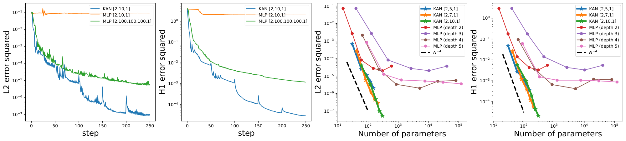
We compare the KAN architecture with that of MLPs using the same hyperparameters $n_i=10000$, $n_b=800$, and $\alpha=0.01$. We measure both the error in the $L^2$ norm and energy ($H^1$) norm and see that KAN achieves a much better scaling law with a smaller error, using smaller networks and fewer parameters; see Figure 8. A 2-Layer width-10 KAN is 100 times more accurate than a 4-Layer width-100 MLP ($10^{-7}$ vs $10^{-5}$ MSE) and 100 times more parameter efficient ($10^2$ vs $10^4$ parameters). Therefore we speculate that KANs might have the potential of serving as a good neural network representation for model reduction of PDEs. However, we want to note that our implementation of KANs are typically 10x slower than MLPs to train. The ground truth being a symbolic formula might be an unfair comparison for MLPs since KANs are good at representing symbolic formulas. In general, KANs and MLPs are good at representing different function classes of PDE solutions, which needs detailed future study to understand their respective boundaries.

3.5 Continual Learning

Catastrophic forgetting is a serious problem in current machine learning [40]. When a human masters a task and switches to another task, they do not forget how to perform the first task. Unfortunately, this is not the case for neural networks. When a neural network is trained on task 1 and then shifted to being trained on task 2, the network will soon forget about how to perform task 1. A key difference between artificial neural networks and human brains is that human brains have functionally distinct modules placed locally in space. When a new task is learned, structure re-organization only occurs in local regions responsible for relevant skills [41, 42], leaving other regions intact. Most artificial neural networks, including MLPs, do not have this notion of locality, which is probably the reason for catastrophic forgetting.

We show that KANs have local plasticity and can avoid catastrophic forgetting by leveraging the locality of splines. The idea is simple: since spline bases are local, a sample will only affect a few nearby spline coefficients, leaving far-away coefficients intact (which is desirable since far-away regions may have already stored information that we want to preserve). By contrast, since MLPs usually use global activations, e.g., ReLU/Tanh/SiLU etc., any local change may propagate uncontrollably to regions far away, destroying the information being stored there.

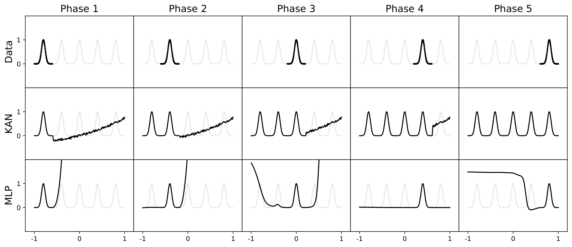
We use a toy example to validate this intuition. The 1D regression task is composed of 5 Gaussian peaks. Data around each peak is presented sequentially (instead of all at once) to KANs and MLPs, as shown in Figure 9 top row. KAN and MLP predictions after each training phase are shown in the middle and bottom rows. As expected, KAN only remodels regions where data is present on in the current phase, leaving previous regions unchanged. By contrast, MLPs remodels the whole region after seeing new data samples, leading to catastrophic forgetting.

Here we simply present our preliminary results on an extremely simple example, to demonstrate how one could possibly leverage locality in KANs (thanks to spline parametrizations) to reduce catastrophic forgetting. However, it remains unclear whether our method can generalize to more realistic setups, especially in high-dimensional cases where it is unclear how to define "locality". In future work, We would also like to study how our method can be connected to and combined with SOTA methods in continual learning [43, 44].

4. KANs are interpretable

Section Summary: This section explains how Kolmogorov-Arnold Networks (KANs) are interpretable, meaning they can reveal the underlying math and structures in data, thanks to special techniques that make them user-friendly and insightful. On simple test problems, KANs accurately learn and display formulas for tasks like multiplication, division, and even complex patterns such as phase changes or special math functions, often simplifying into clear, visual graphs. Beyond these examples, KANs apply to real science, rediscovering tricky relationships in knot theory and physics phase transitions, positioning them as a promising tool for AI-driven discoveries due to their blend of precision and clarity.

In this section, we show that KANs are interpretable and interactive thanks to the techniques we developed in Section 2.5. We want to test the use of KANs not only on synthetic tasks (Section 4.1 and Section 4.2), but also in real-life scientific research. We demonstrate that KANs can (re)discover both highly non-trivial relations in knot theory (Section 4.3) and phase transition boundaries in condensed matter physics (Section 4.4). KANs could potentially be the foundation model for AI + Science due to their accuracy (last section) and interpretability (this section).

4.1 Supervised toy datasets

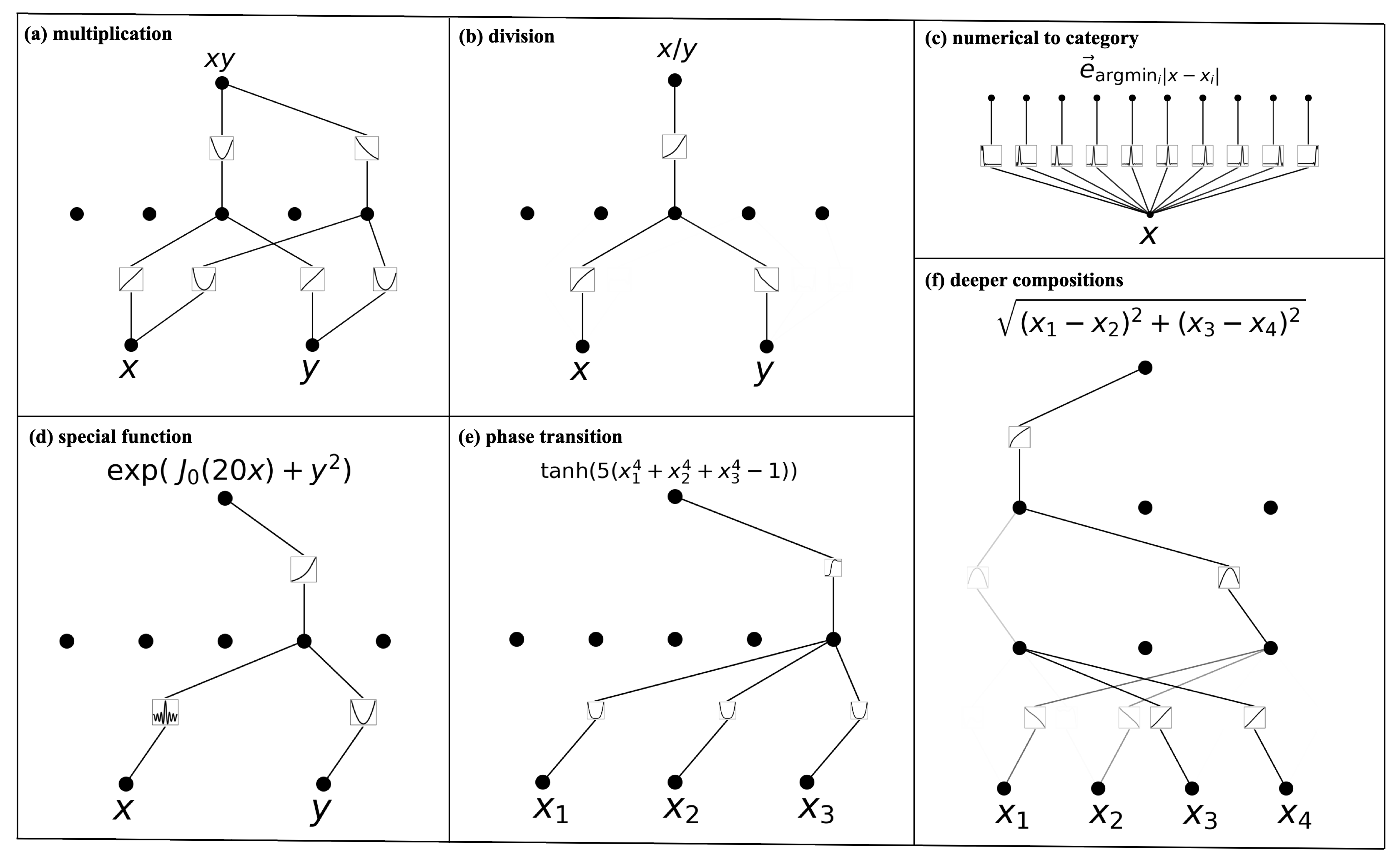
We first examine KANs' ability to reveal the compositional structures in symbolic formulas. Six examples are listed below and their KANs are visualized in Figure 10. KANs are able to reveal the compositional structures present in these formulas, as well as learn the correct univariate functions.

• (a) Multiplication $f(x, y)=xy$. A $[2, 5, 1]$ KAN is pruned to a $[2, 2, 1]$ KAN. The learned activation functions are linear and quadratic. From the computation graph, we see that the way it computes $xy$ is leveraging $2xy=(x+y)^2-(x^2+y^2)$.
• (b) Division of positive numbers $f(x, y)=x/y$. A $[2, 5, 1]$ KAN is pruned to a $[2, 1, 1]$ KAN. The learned activation functions are logarithmic and exponential functions, and the KAN is computing $x/y$ by leveraging the identity $x/y={\exp}({\log}x-{\log}y)$.
• (c) Numerical to categorical. The task is to convert a real number in $[0, 1]$ to its first decimal digit (as one hots), e.g., $0.0618\to [1, 0, 0, 0, 0, \cdots]$, $0.314\to [0, 0, 0, 1, 0, \cdots]$. Notice that activation functions are learned to be spikes located around the corresponding decimal digits.
• (d) Special function $f(x, y)={\rm exp}(J_0(20x)+y^2)$. One limitation of symbolic regression is that it will never find the correct formula of a special function if the special function is not provided as prior knowledge. KANs can learn special functions – the highly wiggly Bessel function $J_0(20x)$ is learned (numerically) by KAN.
• (e) Phase transition $f(x_1, x_2, x_3)={\rm tanh}(5(x_1^4+x_2^4+x_3^4-1))$. Phase transitions are of great interest in physics, so we want KANs to be able to detect phase transitions and to identify the correct order parameters. We use the tanh function to simulate the phase transition behavior, and the order parameter is the combination of the quartic terms of $x_1, x_2, x_3$. Both the quartic dependence and tanh dependence emerge after KAN training. This is a simplified case of a localization phase transition discussed in Section 4.4.
• (f) Deeper compositions $f(x_1, x_2, x_3, x_4)=\sqrt{(x_1-x_2)^2+(x_3-x_4)^2}$. To compute this, we would need the identity function, squared function, and square root, which requires at least a three-layer KAN. Indeed, we find that a $[4, 3, 3, 1]$ KAN can be auto-pruned to a $[4, 2, 1, 1]$ KAN, which exactly corresponds to the computation graph we would expect.

More examples from the Feynman dataset and the special function dataset are visualized in Figure 22, Figure 23, Figure 24, Figure 25 in Appendix D and Appendix F.

4.2 Unsupervised toy dataset

Often, scientific discoveries are formulated as supervised learning problems, i.e., given input variables $x_1, x_2, \cdots, x_d$ and output variable(s) $y$, we want to find an interpretable function $f$ such that $y\approx f(x_1, x_2, \cdots, x_d)$. However, another type of scientific discovery can be formulated as unsupervised learning, i.e., given a set of variables $(x_1, x_2, \cdots, x_d)$, we want to discover a structural relationship between the variables. Specifically, we want to find a non-zero $f$ such that

$ \begin{align} f(x_1, x_2, \cdots, x_d)\approx 0. \end{align} $

For example, consider a set of features $(x_1, x_2, x_3)$ that satisfies $x_3={\rm exp}({\rm sin}(\pi x_1)+x_2^2)$. Then a valid $f$ is $f(x_1, x_2, x_3)={\rm sin}(\pi x_1)+x_2^2-{\rm log}(x_3)=0$, implying that points of $(x_1, x_2, x_3)$ form a 2D submanifold specified by $f=0$ instead of filling the whole 3D space.

If an algorithm for solving the unsupervised problem can be devised, it has a considerable advantage over the supervised problem, since it requires only the sets of features $S=(x_1, x_2, \cdots, x_d)$. The supervised problem, on the other hand, tries to predict subsets of features in terms of the others, i.e. it splits $S=S_\text{in} \cup S_\text{out}$ into input and output features of the function to be learned. Without domain expertise to advise the splitting, there are $2^d-2$ possibilities such that $|S_\text{in}|>0$ and $|S_\text{out}|>0$. This exponentially large space of supervised problems can be avoided by using the unsupervised approach. This unsupervised learning approach will be valuable to the knot dataset in Section 4.3. A Google Deepmind team [45] manually chose signature to be the target variable, otherwise they would face this combinatorial problem described above. This raises the question whether we can instead tackle the unsupervised learning directly. We present our method and a toy example below.

We tackle the unsupervised learning problem by turning it into a supervised learning problem on all of the $d$ features, without requiring the choice of a splitting. The essential idea is to learn a function $f(x_1, \dots, x_d)=0$ such that $f$ is not the $0$-function. To do this, similar to contrastive learning, we define positive samples and negative samples: positive samples are feature vectors of real data. Negative samples are constructed by feature corruption. To ensure that the overall feature distribution for each topological invariant stays the same, we perform feature corruption by random permutation of each feature across the entire training set. Now we want to train a network $g$ such that $g(\mathbf{x}{\rm real})=1$ and $g(\mathbf{x}{\rm fake})=0$ which turns the problem into a supervised problem. However, remember that we originally want $f(\mathbf{x}{\rm real})=0$ and $f(\mathbf{x}{\rm fake})\neq 0$. We can achieve this by having $g=\sigma\circ f$ where $\sigma(x)={\rm exp}(-\frac{x^2}{2w^2})$ is a Gaussian function with a small width $w$, which can be conveniently realized by a KAN with shape $[..., 1, 1]$ whose last activation is set to be the Gaussian function $\sigma$ and all previous layers form $f$. Except for the modifications mentioned above, everything else is the same for supervised training.

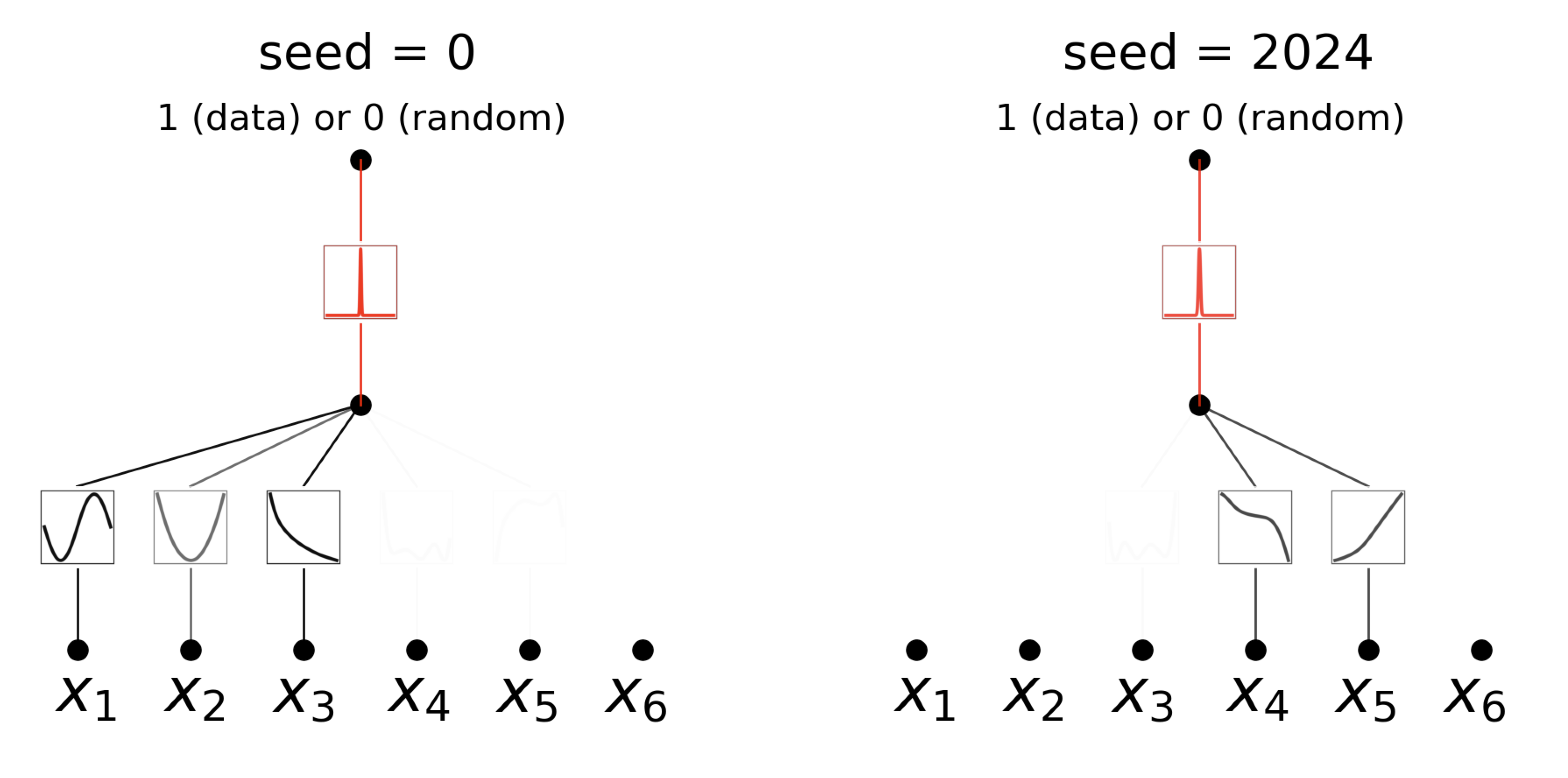
Now we demonstrate that the unsupervised paradigm works for a synthetic example. Let us consider a 6D dataset, where $(x_1, x_2, x_3)$ are dependent variables such that $x_3=\exp(\sin(x_1)+x_2^2)$; $(x_4, x_5)$ are dependent variables with $x_5=x_4^3$; $x_6$ is independent of the other variables. In Figure 11, we show that for seed = 0, KAN reveals the functional dependence among $x_1$, $x_2$, and $x_3$; for another seed = 2024, KAN reveals the functional dependence between $x_4$ and $x_5$. Our preliminary results rely on randomness (different seeds) to discover different relations; in the future we would like to investigate a more systematic and more controlled way to discover a complete set of relations. Even so, our tool in its current status can provide insights for scientific tasks. We present our results with the knot dataset in Section 4.3.

4.3 Application to Mathematics: Knot Theory

Knot theory is a subject in low-dimensional topology that sheds light on topological aspects of three-manifolds and four-manifolds and has a variety of applications, including in biology and topological quantum computing. Mathematically, a knot $K$ is an embedding of $S^1$ into $S^3$. Two knots $K$ and $K'$ are topologically equivalent if one can be deformed into the other via deformation of the ambient space $S^3$, in which case we write $[K]=[K']$. Some knots are topologically trivial, meaning that they can be smoothly deformed to a standard circle. Knots have a variety of deformation-invariant features $f$ called topological invariants, which may be used to show that two knots are topologically inequivalent, $[K]\neq [K']$ if $f(K) \neq f(K')$. In some cases the topological invariants are geometric in nature. For instance, a hyperbolic knot $K$ has a knot complement $S^3\setminus K$ that admits a canonical hyperbolic metric $g$ such that $\text{vol}_g(K)$ is a topological invariant known as the hyperbolic volume. Other topological invariants are algebraic in nature, such as the Jones polynomial.

Given the fundamental nature of knots in mathematics and the importance of its applications, it is interesting to study whether ML can lead to new results. For instance, in [46] reinforcement learning was utilized to establish ribbonness of certain knots, which ruled out many potential counterexamples to the smooth 4d Poincaré conjecture.

Supervised learning In [45], supervised learning and human domain experts were utilized to arrive at a new theorem relating algebraic and geometric knot invariants. In this case, gradient saliency identified key invariants for the supervised problem, which led the domain experts to make a conjecture that was subsequently refined and proven. We study whether a KAN can achieve good interpretable results on the same problem, which predicts the signature of a knot. Their main results from studying the knot theory dataset are:

• (1) They use network attribution methods to find that the signature $\sigma$ is mostly dependent on meridinal distance $\mu$ (real $\mu_r$, imag $\mu_i$) and longitudinal distance $\lambda$.
• (2) Human scientists later identified that $\sigma$ has high correlation with the ${\rm slope}\equiv {\rm Re}(\frac{\lambda}{\mu})=\frac{\lambda\mu_r}{\mu_r^2+\mu_i^2}$ and derived a bound for $|2\sigma-{\rm slope}|$.

We show below that KANs not only rediscover these results with much smaller networks and much more automation, but also present some interesting new results and insights.

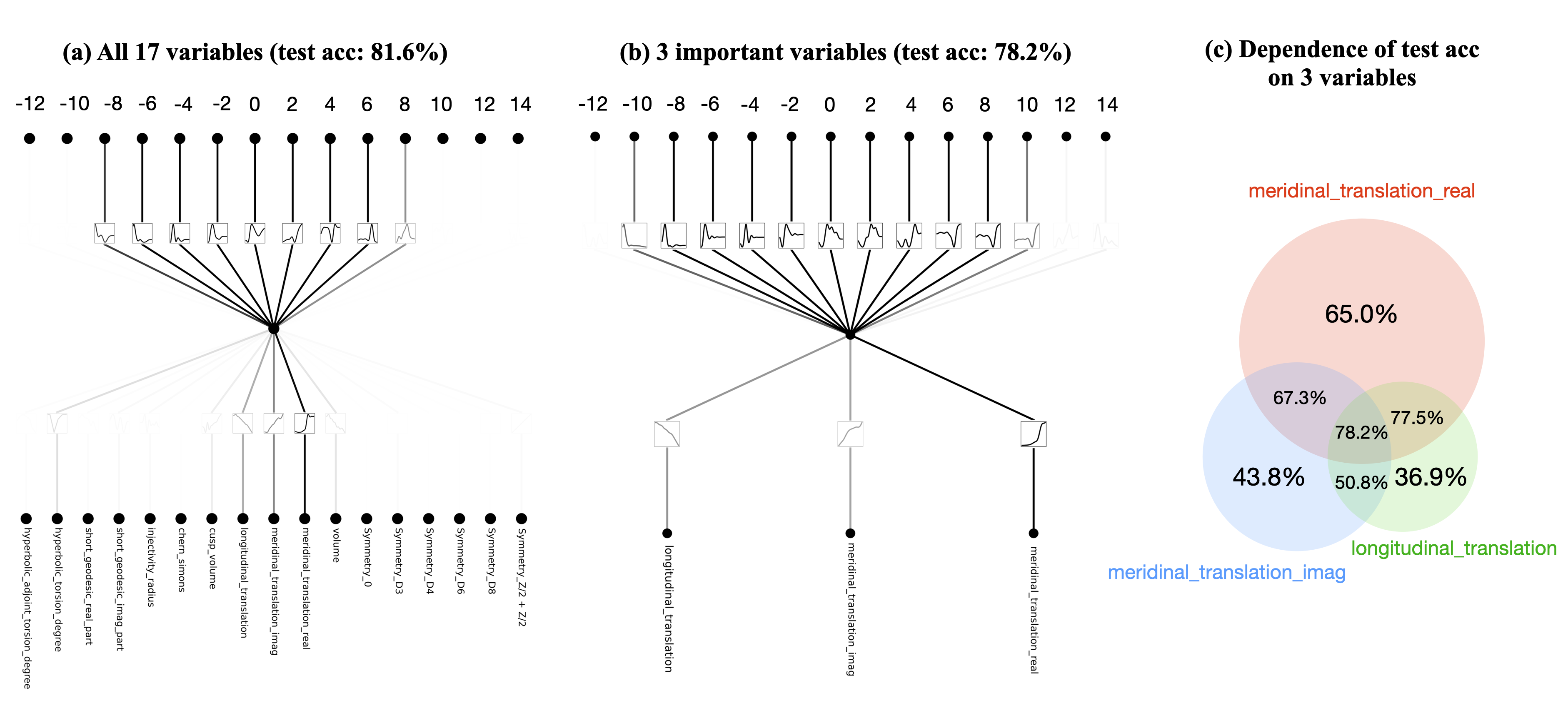
To investigate (1), we treat 17 knot invariants as inputs and signature as outputs. Similar to the setup in [45], signatures (which are even numbers) are encoded as one-hot vectors and networks are trained with cross-entropy loss. We find that an extremely small $[17, 1, 14]$ KAN is able to achieve $81.6%$ test accuracy (while Deepmind's 4-layer width-300 MLP achieves 78% test accuracy). The $[17, 1, 14]$ KAN ($G=3$, $k=3$) has $\approx 200$ parameters, while the MLP has $\approx 3\times 10^5$ parameters, shown in Table 3. It is remarkable that KANs can be both more accurate and much more parameter efficient than MLPs at the same time. In terms of interpretability, we scale the transparency of each activation according to its magnitude, so it becomes immediately clear which input variables are important without the need for feature attribution (see Figure 12 left): signature is mostly dependent on $\mu_r$, and slightly dependent on $\mu_i$ and $\lambda$, while dependence on other variables is small. We then train a $[3, 1, 14]$ KAN on the three important variables, obtaining test accuracy $78.2%$. Our results have one subtle difference from results in [45]: they find that signature is mostly dependent on $\mu_i$, while we find that signature is mostly dependent on $\mu_r$. This difference could be due to subtle algorithmic choices, but has led us to carry out the following experiments: (a) ablation studies. We show that $\mu_r$ contributes more to accuracy than $\mu_i$ (see Figure 12): for example, $\mu_r$ alone can achieve $65.0%$ accuracy, while $\mu_i$ alone can only achieve $43.8%$ accuracy. (b) We find a symbolic formula (in Table 4) which only involves $\mu_r$ and $\lambda$, but can achieve $77.8%$ test accuracy.

: Table 3: KANs can achieve better accuracy than MLPs with much fewer parameters in the signature classification problem. Soon after our preprint was first released, Prof. Shi Lab from Georgia tech discovered that an MLP with only 60 parameters is sufficient to achieve 80% accuracy (public but unpublished results). This is good news for AI + Science because this means perhaps many AI + Science tasks are not that computationally demanding than we might think (either with MLPs or with KANs), hence many new scientific discoveries are possible even on personal laptops.

Method	Architecture	Parameter Count	Accuracy
Deepmind's MLP	4 layer, width-300	$3\times 10^5$	$78.0%$
KANs	2 layer, $[17, 1, 14]$ ($G=3$, $k=3$)	$2\times 10^2$	$81.6%$

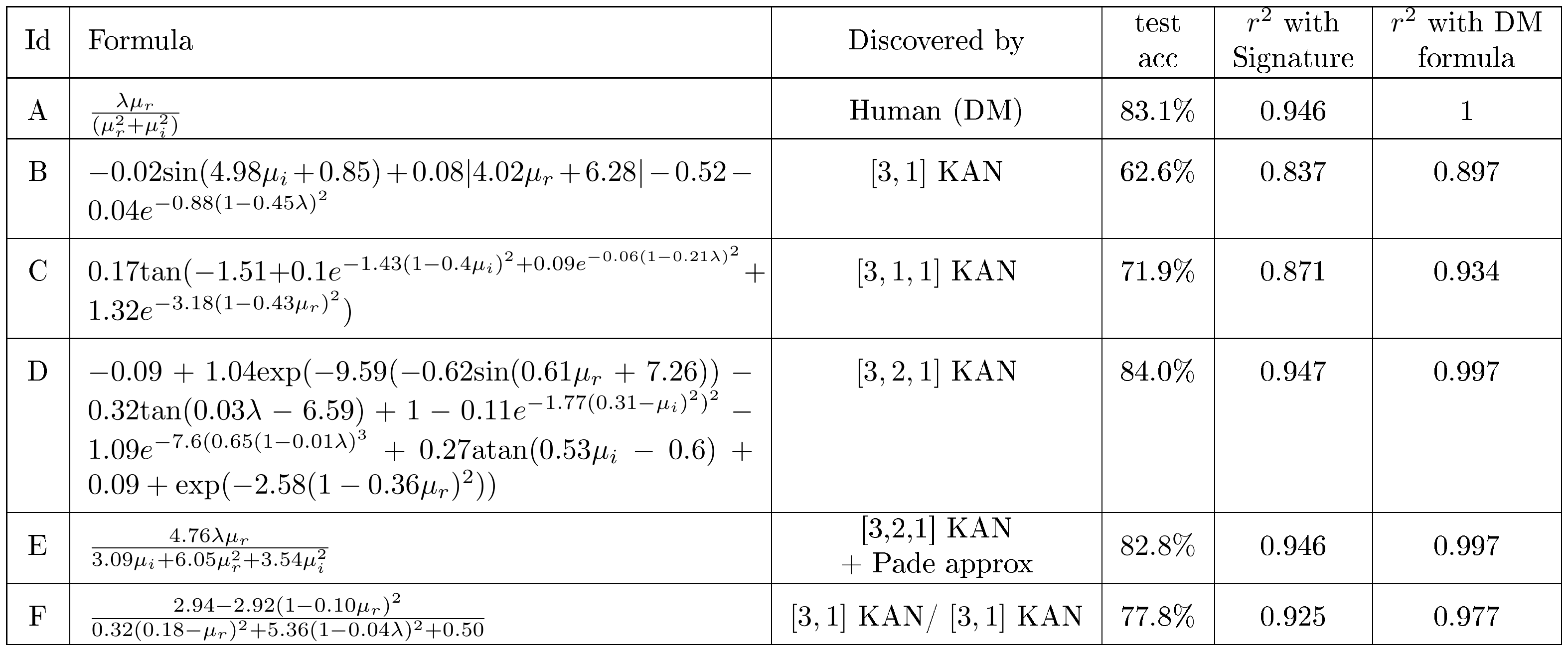
To investigate (2), i.e., obtain the symbolic form of $\sigma$, we formulate the problem as a regression task. Using auto-symbolic regression introduced in Section 2.5.1, we can convert a trained KAN into symbolic formulas. We train KANs with shapes $[3, 1]$, $[3, 1, 1]$, $[3, 2, 1]$, whose corresponding symbolic formulas are displayed in Table 4 B-D. It is clear that by having a larger KAN, both accuracy and complexity increase. So KANs provide not just a single symbolic formula, but a whole Pareto frontier of formulas, trading off simplicity and accuracy. However, KANs need additional inductive biases to further simplify these equations to rediscover the formula from [45] (Table 4 A). We have tested two scenarios: (1) in the first scenario, we assume the ground truth formula has a multi-variate Pade representation (division of two multi-variate Taylor series). We first train $[3, 2, 1]$ and then fit it to a Pade representation. We can obtain Formula E in Table 4, which bears similarity with Deepmind's formula. (2) We hypothesize that the division is not very interpretable for KANs, so we train two KANs (one for the numerator and the other for the denominator) and divide them manually. Surprisingly, we end up with the formula F (in Table 4) which only involves $\mu_r$ and $\lambda$, although $\mu_i$ is also provided but ignored by KANs.

::: {caption="Table 4: Symbolic formulas of signature as a function of meridinal translation $\mu$ (real $\mu_r$, imag $\mu_i$) and longitudinal translation $\lambda$. In [45], formula A was discovered by human scientists inspired by neural network attribution results. Formulas B-F are auto-discovered by KANs. KANs can trade-off between simplicity and accuracy (B, C, D). By adding more inductive biases, KAN is able to discover formula E which is not too dissimilar from formula A. KANs also discovered a formula F which only involves two variables ($\mu_r$ and $\lambda$) instead of all three variables, with little sacrifice in accuracy."}

:::

So far, we have rediscovered the main results from [45]. It is remarkable to see that KANs made this discovery very intuitive and convenient. Instead of using feature attribution methods (which are great methods), one can instead simply stare at visualizations of KANs. Moreover, automatic symbolic regression also makes the discovery of symbolic formulas much easier.

In the next part, we propose a new paradigm of "AI for Math" not included in the Deepmind paper, where we aim to use KANs' unsupervised learning mode to discover more relations (besides signature) in knot invariants.

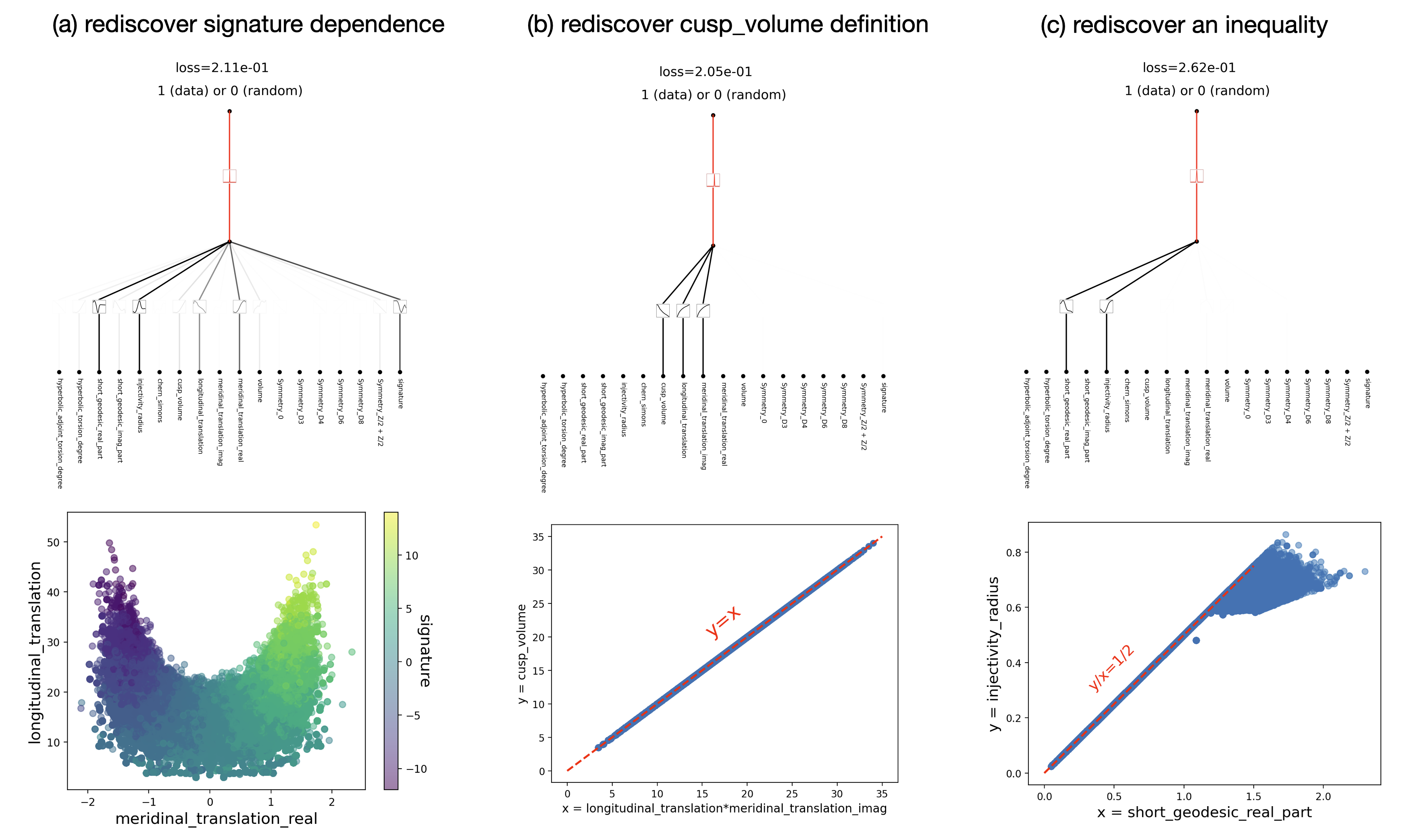
Unsupervised learning As we mentioned in Section 4.2, unsupervised learning is the setup that is more promising since it avoids manual partition of input and output variables which have combinatorially many possibilities. In the unsupervised learning mode, we treat all 18 variables (including signature) as inputs such that they are on the same footing. Knot data are positive samples, and we randomly shuffle features to obtain negative samples. An $[18, 1, 1]$ KAN is trained to classify whether a given feature vector belongs to a positive sample (1) or a negative sample (0). We manually set the second layer activation to be the Gaussian function with a peak one centered at zero, so positive samples will have activations at (around) zero, implicitly giving a relation among knot invariants $\sum_{i=1}^{18} g_i(x_i)=0$ where $x_i$ stands for a feature (invariant), and $g_i$ is the corresponding activation function which can be readily read off from KAN diagrams. We train the KANs with $\lambda={10^{-2}, 10^{-3}}$ to favor sparse combination of inputs, and ${\rm seed}={0, 1, \cdots, 99}$. All 200 networks can be grouped into three clusters, with representative KANs displayed in Figure 13. These three groups of dependent variables are:

• (1) The first group of dependent variables is signature, real part of meridinal distance, and longitudinal distance (plus two other variables which can be removed because of (3)). This is the signature dependence studied above, so it is very interesting to see that this dependence relation is rediscovered again in the unsupervised mode.
• (2) The second group of variables involve cusp volume $V$, real part of meridinal translation $\mu_r$ and longitudinal translation $\lambda$. Their activations all look like logarithmic functions (which can be verified by the implied symbolic functionality in Section 2.5.1). So the relation is $-\log V+\log \mu_r+\log \lambda=0$ which is equivalent to $V=\mu_r\lambda$, which is true by definition. It is, however, reassuring that we discover this relation without any prior knowledge.
• (3) The third group of variables includes the real part of short geodesic $g_r$ and injectivity radius. Their activations look qualitatively the same but differ by a minus sign, so it is conjectured that these two variables have a linear correlation. We plot 2D scatters, finding that $2r$ upper bounds $g_r$, which is also a well-known relation [47].

It is interesting that KANs' unsupervised mode can rediscover several known mathematical relations. The good news is that the results discovered by KANs are probably reliable; the bad news is that we have not discovered anything new yet. It is worth noting that we have chosen a shallow KAN for simple visualization, but deeper KANs can probably find more relations if they exist. We would like to investigate how to discover more complicated relations with deeper KANs in future work.

4.4 Application to Physics: Anderson localization

Anderson localization is the fundamental phenomenon in which disorder in a quantum system leads to the localization of electronic wave functions, causing all transport to be ceased [48]. In one and two dimensions, scaling arguments show that all electronic eigenstates are exponentially localized for an infinitesimal amount of random disorder [49, 50]. In contrast, in three dimensions, a critical energy forms a phase boundary that separates the extended states from the localized states, known as a mobility edge. The understanding of these mobility edges is crucial for explaining various fundamental phenomena such as the metal-insulator transition in solids [51], as well as localization effects of light in photonic devices [52, 53, 54, 55, 56]. It is therefore necessary to develop microscopic models that exhibit mobility edges to enable detailed investigations. Developing such models is often more practical in lower dimensions, where introducing quasiperiodicity instead of random disorder can also result in mobility edges that separate localized and extended phases. Furthermore, experimental realizations of analytical mobility edges can help resolve the debate on localization in interacting systems [57, 58]. Indeed, several recent studies have focused on identifying such models and deriving exact analytic expressions for their mobility edges [59, 60, 61, 62, 63, 64, 65].

Here, we apply KANs to numerical data generated from quasiperiodic tight-binding models to extract their mobility edges. In particular, we examine three classes of models: the Mosaic model (MM) [63], the generalized Aubry-André model (GAAM) [62] and the modified Aubry-André model (MAAM) [60]. For the MM, we testify KAN's ability to accurately extract mobility edge as a 1D function of energy. For the GAAM, we find that the formula obtained from a KAN closely matches the ground truth. For the more complicated MAAM, we demonstrate yet another example of the symbolic interpretability of this framework. A user can simplify the complex expression obtained from KANs (and corresponding symbolic formulas) by means of a "collaboration" where the human generates hypotheses to obtain a better match (e.g., making an assumption of the form of certain activation function), after which KANs can carry out quick hypotheses testing.

To quantify the localization of states in these models, the inverse participation ratio (IPR) is commonly used. The IPR for the $k^{th}$ eigenstate, $\psi^{(k)}$, is given by

$ \begin{align} \text{IPR}_k = \frac{\sum_n |\psi^{(k)}_n|^4}{\left(\sum_n |\psi^{(k)}_n|^2\right)^2} \end{align} $

where the sum runs over the site index. Here, we use the related measure of localization – the fractal dimension of the states, given by

$ \begin{align} D_k = -\frac{\log(\text{IPR}_k)}{\log(N)} \end{align} $

where $N$ is the system size. $D_k = 0 (1)$ indicates localized (extended) states.

Mosaic Model (MM) We first consider a class of tight-binding models defined by the Hamiltonian [63]

$ \begin{align} H = t\sum_n \left(c^\dag_{n+1} c_n + \text{H.c.}\right) + \sum_n V_n(\lambda, \phi) c^\dag_n c_n, \end{align} $

where $t$ is the nearest-neighbor coupling, $c_n (c^\dag_n)$ is the annihilation (creation) operator at site $n$ and the potential energy $V_n$ is given by

$ \begin{align} V_n(\lambda, \phi) = \begin{cases} \lambda\cos(2\pi nb + \phi) & j = m\kappa\ 0, & \text{otherwise, } \end{cases} \end{align} $

To introduce quasiperiodicity, we set $b$ to be irrational (in particular, we choose $b$ to be the golden ratio $\frac{1+\sqrt{5}}{2}$). $\kappa$ is an integer and the quasiperiodic potential occurs with interval $\kappa$. The energy ($E$) spectrum for this model generically contains extended and localized regimes separated by a mobility edge. Interestingly, a unique feature found here is that the mobility edges are present for an arbitrarily strong quasiperiodic potential (i.e. there are always extended states present in the system that co-exist with localized ones).

The mobility edge can be described by $g(\lambda, E)\equiv\lambda-|f_\kappa(E)|=0$. $g(\lambda, E)$ > 0 and $g(\lambda, E)$ < 0 correspond to localized and extended phases, respectively. Learning the mobility edge therefore hinges on learning the "order parameter" $g(\lambda, E)$. Admittedly, this problem can be tackled by many other theoretical methods for this class of models [63], but we will demonstrate below that our KAN framework is ready and convenient to take in assumptions and inductive biases from human users.

Let us assume a hypothetical user Alice, who is a new PhD student in condensed matter physics, and she is provided with a $[2, 1]$ KAN as an assistant for the task. Firstly, she understands that this is a classification task, so it is wise to set the activation function in the second layer to be sigmoid by using the fix_symbolic functionality. Secondly, she realizes that learning the whole 2D function $g(\lambda, E)$ is unnecessary because in the end she only cares about $\lambda=\lambda(E)$ determined by $g(\lambda, E)=0$. In so doing, it is reasonable to assume $g(\lambda, E)=\lambda-h(E)=0$. Alice simply sets the activation function of $\lambda$ to be linear by again using the fix_symbolic functionality. Now Alice trains the KAN network and conveniently obtains the mobility edge, as shown in Figure 14. Alice can get both intuitive qualitative understanding (bottom) and quantitative results (middle), which well match the ground truth (top).

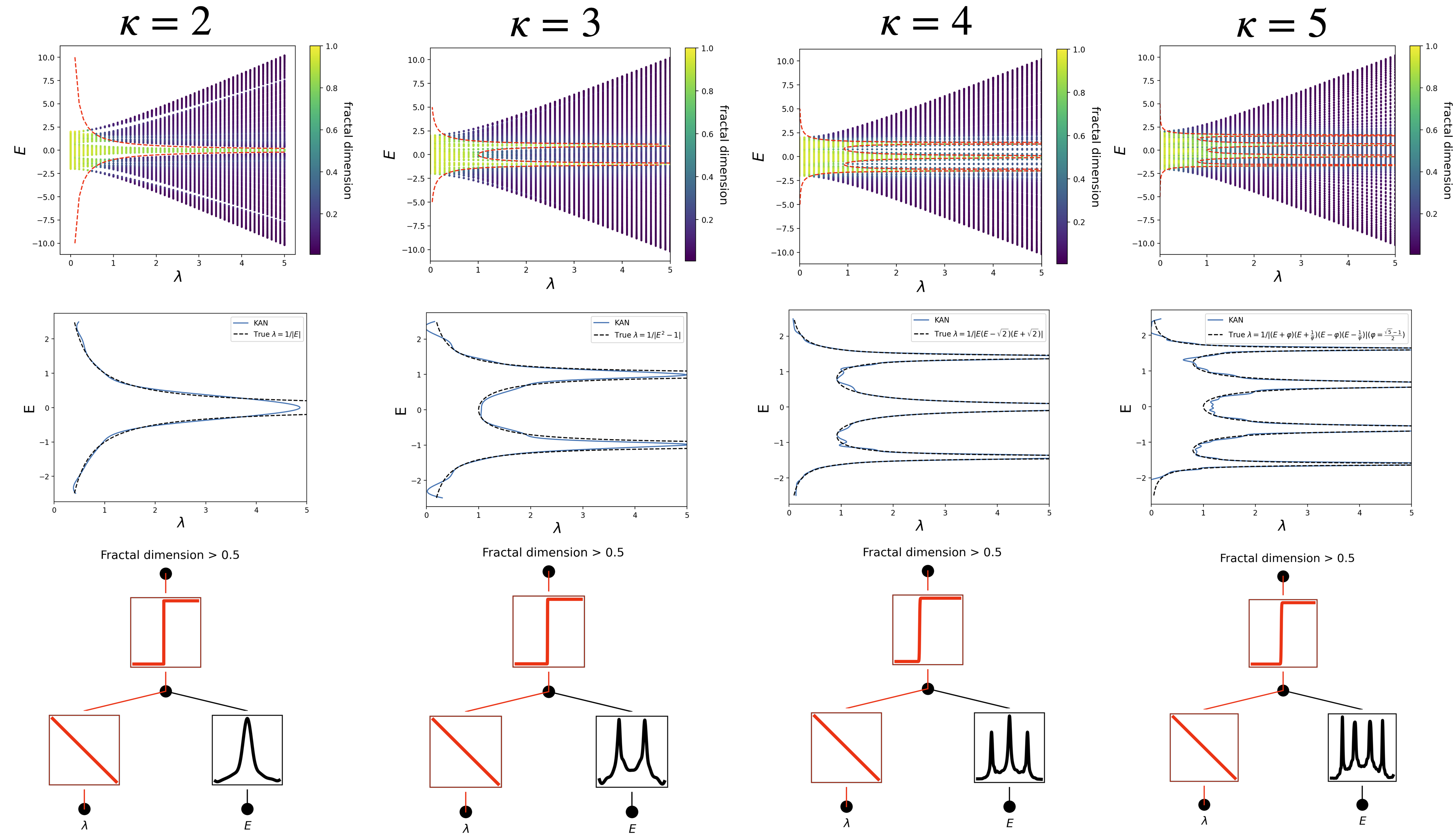
Generalized Andre-Aubry Model (GAAM) We next consider a class of tight-binding models defined by the Hamiltonian [62]

$ \begin{align} H = t\sum_n \left(c^\dag_{n+1} c_n + \text{H.c.}\right) + \sum_n V_n(\alpha, \lambda, \phi) c^\dag_n c_n, \end{align} $

where $t$ is the nearest-neighbor coupling, $c_n (c^\dag_n)$ is the annihilation (creation) operator at site $n$ and the potential energy $V_n$ is given by

$ \begin{align} V_n(\alpha, \lambda, \phi) = 2\lambda \frac{\cos(2\pi n b + \phi)}{1-\alpha \cos(2\pi n b + \phi)}, \end{align} $

which is smooth for $\alpha \in (-1, 1)$. To introduce quasiperiodicity, we again set $b$ to be irrational (in particular, we choose $b$ to be the golden ratio). As before, we would like to obtain an expression for the mobility edge. For these models, the mobility edge is given by the closed form expression [62, 64],

$ \begin{align} \alpha E = 2(t-\lambda). \end{align}\tag{6} $

We randomly sample the model parameters: $\phi$, $\alpha$ and $\lambda$ (setting the energy scale $t=1$) and calculate the energy eigenvalues as well as the fractal dimension of the corresponding eigenstates, which forms our training dataset.

::: {caption="Table 5: Symbolic formulas for two systems GAAM and MAAM, ground truth ones and KAN-discovered ones."}

:::

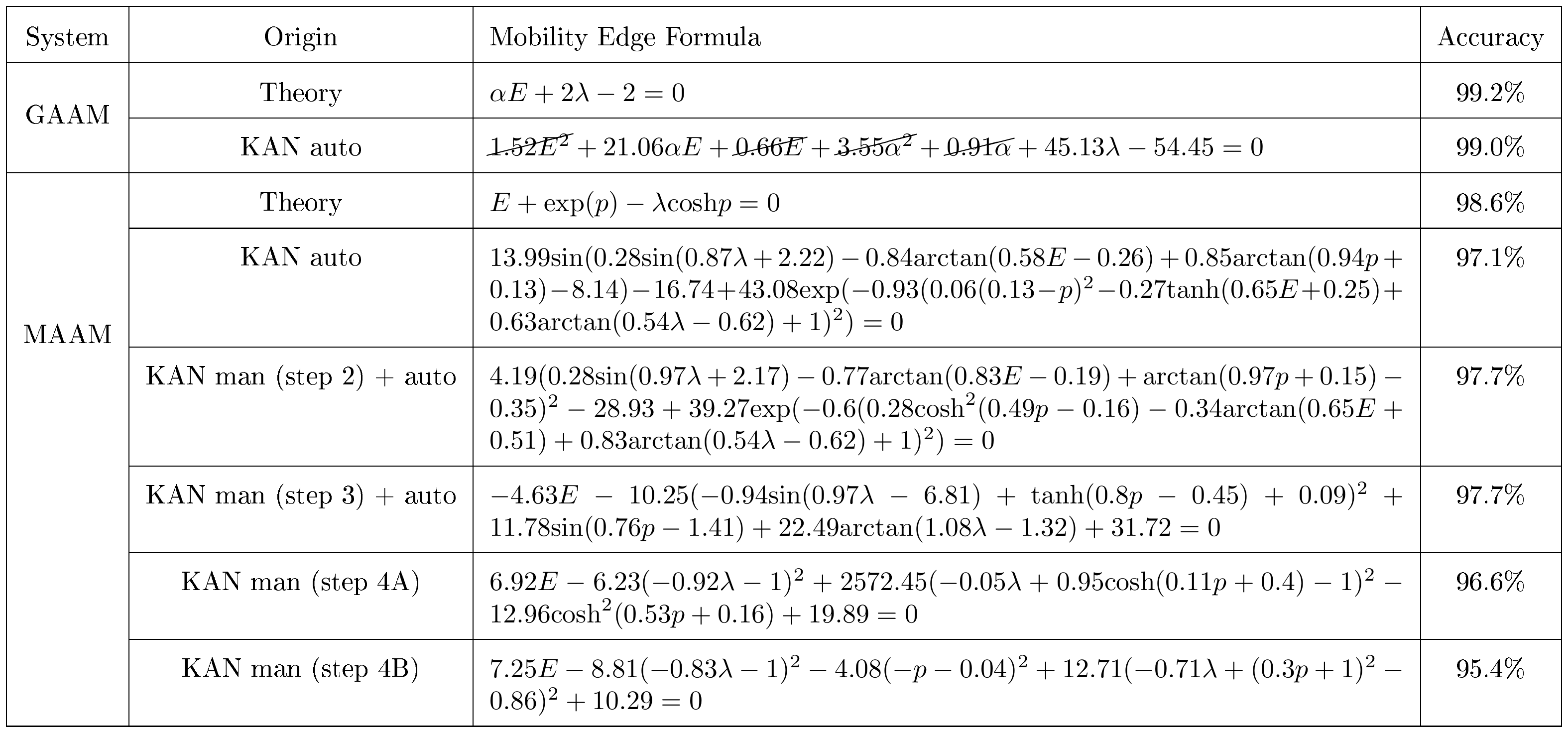
Here the "order parameter" to be learned is $g(\alpha, E, \lambda, \phi)=\alpha E+2(\lambda -1)$ and mobility edge corresponds to $g=0$. Let us again assume that Alice wants to figure out the mobility edge but only has access to IPR or fractal dimension data, so she decides to use KAN to help her with the task. Alice wants the model to be as small as possible, so she could either start from a large model and use auto-pruning to get a small model, or she could guess a reasonable small model based on her understanding of the complexity of the given problem. Either way, let us assume she arrives at a $[4, 2, 1, 1]$ KAN. First, she sets the last activation to be sigmoid because this is a classification problem. She trains her KAN with some sparsity regularization to accuracy 98.7% and visualizes the trained KAN in Figure 15 (a) step 1. She observes that $\phi$ is not picked up on at all, which makes her realize that the mobility edge is independent of $\phi$ (agreeing with Eq. (6)). In addition, she observes that almost all other activation functions are linear or quadratic, so she turns on automatic symbolic snapping, constraining the library to be only linear or quadratic. After that, she immediately gets a network which is already symbolic (shown in Figure 15 (a) step 2), with comparable (even slightly better) accuracy 98.9%. By using symbolic_formula functionality, Alice conveniently gets the symbolic form of $g$, shown in Table 5 GAAM-KAN auto (row three). Perhaps she wants to cross out some small terms and snap coefficient to small integers, which takes her close to the true answer.

This hypothetical story for Alice would be completely different if she is using a symbolic regression method. If she is lucky, SR can return the exact correct formula. However, the vast majority of the time SR does not return useful results and it is impossible for Alice to "debug" or interact with the underlying process of symbolic regression. Furthermore, Alice may feel uncomfortable/inexperienced to provide a library of symbolic terms as prior knowledge to SR before SR is run. By constrast in KANs, Alice does not need to put any prior information to KANs. She can first get some clues by staring at a trained KAN and only then it is her job to decide which hypothesis she wants to make (e.g., "all activations are linear or quadratic") and implement her hypothesis in KANs. Although it is not likely for KANs to return the correct answer immediately, KANs will always return something useful, and Alice can collaborate with it to refine the results.

Modified Andre-Aubry Model (MAAM) The last class of models we consider is defined by the Hamiltonian [60]

$ \begin{align} H = \sum_{n\ne n'} te^{-p|n-n'|}\left(c^\dag_{n} c_{n'} + \text{H.c.}\right) + \sum_n V_n(\lambda, \phi) c^\dag_n c_n, \end{align} $

where $t$ is the strength of the exponentially decaying coupling in space, $c_n (c^\dag_n)$ is the annihilation (creation) operator at site $n$ and the potential energy $V_n$ is given by

$ \begin{align} V_n(\lambda, \phi) = \lambda \cos(2\pi n b + \phi), \end{align} $

As before, to introduce quasiperiodicity, we set $b$ to be irrational (the golden ratio). For these models, the mobility edge is given by the closed form expression [60],

$ \begin{align} \lambda \cosh(p) = E + t = E + t_1{\rm exp}(p) \end{align}\tag{7} $

where we define $t_1\equiv t{\rm exp}(-p)$ as the nearest neighbor hopping strength, and we set $t_1=1$ below.

Let us assume Alice wants to figure out the mobility edge for MAAM. This task is more complicated and requires more human wisdom. As in the last example, Alice starts from a $[4, 2, 1, 1]$ KAN and trains it but gets an accuracy around 75% which is less than acceptable. She then chooses a larger $[4, 3, 1, 1]$ KAN and successfully gets 98.4% which is acceptable (Figure 15 (b) step 1). Alice notices that $\phi$ is not picked up on by KANs, which means that the mobility edge is independent of the phase factor $\phi$ (agreeing with Eq. (7)). If Alice turns on the automatic symbolic regression (using a large library consisting of exp, tanh etc.), she would get a complicated formula in Tabel Table 5-MAAM-KAN auto, which has 97.1% accuracy. However, if Alice wants to find a simpler symbolic formula, she will want to use the manual mode where she does the symbolic snapping by herself. Before that she finds that the $[4, 3, 1, 1]$ KAN after training can then be pruned to be $[4, 2, 1, 1]$, while maintaining $97.7%$ accuracy (Figure 15 (b)). Alice may think that all activation functions except those dependent on $p$ are linear or quadratic and snap them to be either linear or quadratic manually by using fix_symbolic. After snapping and retraining, the updated KAN is shown in Figure 15 (c) step 3, maintaining $97.7%$ accuracy. From now on, Alice may make two different choices based on her prior knowledge. In one case, Alice may have guessed that the dependence on $p$ is ${\rm cosh}$, so she sets the activations of $p$ to be ${\rm cosh}$ function. She retrains KAN and gets 96.9% accuracy (Figure 15 (c) Step 4A). In another case, Alice does not know the ${\rm cosh}\ p$ dependence, so she pursues simplicity and again assumes the functions of $p$ to be quadratic. She retrains KAN and gets 95.4% accuracy (Figure 15 (c) Step 4B). If she tried both, she would realize that ${\rm cosh}$ is better in terms of accuracy, while quadratic is better in terms of simplicity. The formulas corresponding to these steps are listed in Table 5. It is clear that the more manual operations are done by Alice, the simpler the symbolic formula is (which slight sacrifice in accuracy). KANs have a "knob" that a user can tune to trade-off between simplicity and accuracy (sometimes simplicity can even lead to better accuracy, as in the GAAM case).

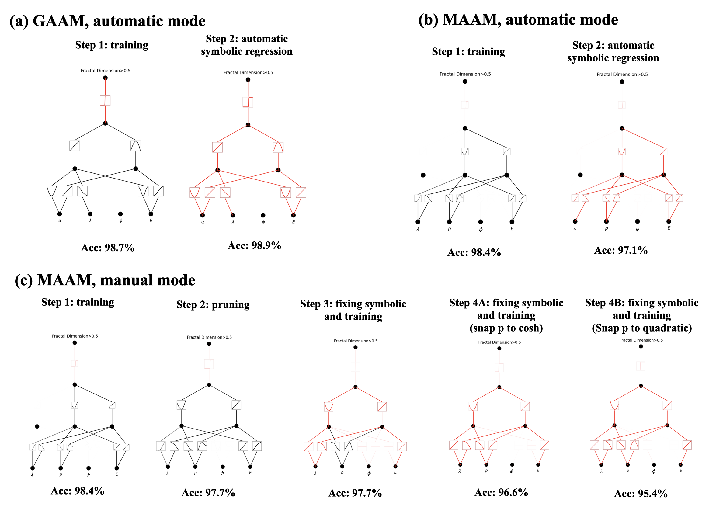
5. Related works

Section Summary: This section reviews prior research linking the Kolmogorov-Arnold theorem to neural networks, noting that while early studies explored this connection, they often relied on limited architectures and toy examples, whereas the current work extends these ideas to more flexible, modern deep learning setups and compares them to models like generalized additive models. It also discusses neural scaling laws, where performance improves predictably with more data or compute, and suggests that smooth representations from this theorem could enable unusually fast progress; mechanistic interpretability efforts to understand neural network workings; learnable activation functions using techniques like splines; symbolic regression methods for discovering mathematical formulas; and physics-informed networks for solving equations, all of which could benefit from the proposed approach. Finally, it touches on AI applications in mathematics, such as analyzing knot theory, highlighting the paper's potential to advance interpretable AI in scientific discovery.

Kolmogorov-Arnold theorem and neural networks. The connection between the Kolmogorov-Arnold theorem (KAT) and neural networks is not new in the literature [66, 67, 9, 10, 11, 12, 13, 14, 68, 69], but the pathological behavior of inner functions makes KAT appear unpromising in practice [66]. Most of these prior works stick to the original 2-layer width-($2n+1$) networks, which were limited in expressive power and many of them are even predating back-propagation. Therefore, most studies were built on theories with rather limited or artificial toy experiments. More broadly speaking, KANs are also somewhat related to generalized additive models (GAMs) [70], graph neural networks [71] and kernel machines [72]. The connections are intriguing and fundamental but might be out of the scope of the current paper. Our contribution lies in generalizing the Kolmogorov network to arbitrary widths and depths, revitalizing and contexualizing them in today's deep learning stream, as well as highlighting its potential role as a foundation model for AI + Science.

Neural Scaling Laws (NSLs). NSLs are the phenomena where test losses behave as power laws against model size, data, compute etc [73, 74, 75, 76, 24, 77, 78, 79]. The origin of NSLs still remains mysterious, but competitive theories include intrinsic dimensionality [73], quantization of tasks [78], resource theory [79], random features [77], compositional sparsity [66], and maximu arity [25]. This paper contributes to this space by showing that a high-dimensional function can surprisingly scale as a 1D function (which is the best possible bound one can hope for) if it has a smooth Kolmogorov-Arnold representation. Our paper brings fresh optimism to neural scaling laws, since it promises the fastest scaling exponent ever. We have shown in our experiments that this fast neural scaling law can be achieved on synthetic datasets, but future research is required to address the question whether this fast scaling is achievable for more complicated tasks (e.g., language modeling): Do KA representations exist for general tasks? If so, does our training find these representations in practice?

Mechanistic Interpretability (MI). MI is an emerging field that aims to mechanistically understand the inner workings of neural networks [80, 81, 82, 83, 84, 85, 86, 87, 5]. MI research can be roughly divided into passive and active MI research. Most MI research is passive in focusing on understanding existing neural networks trained with standard methods. Active MI research attempts to achieve interpretability by designing intrinsically interpretable architectures or developing training methods to explicitly encourage interpretability [86, 87]. Our work lies in the second category, where the model and training method are by design interpretable.

Learnable activations. The idea of learnable activations in neural networks is not new in machine learning. Trainable activations functions are learned in a differentiable way [88, 14, 89, 90] or searched in a discrete way [91]. Activation function are parametrized as polynomials [88], splines [14, 92, 93], sigmoid linear unit [89], or neural networks [90]. KANs use B-splines to parametrize their activation functions. We also present our preliminary results on learnable activation networks (LANs), whose properties lie between KANs and MLPs and their results are deferred to Appendix B to focus on KANs in the main paper.

Symbolic Regression. There are many off-the-shelf symbolic regression methods based on genetic algorithms (Eureka [94], GPLearn [95], PySR [96]), neural-network based methods (EQL [97], OccamNet [98]), physics-inspired method (AI Feynman [36, 37]), and reinforcement learning-based methods [99]. KANs are most similar to neural network-based methods, but differ from previous works in that our activation functions are continuously learned before symbolic snapping rather than manually fixed [94, 98].

Physics-Informed Neural Networks (PINNs) and Physics-Informed Neural Operators (PINOs). In Subsection Section 3.4, we demonstrate that KANs can replace the paradigm of using MLPs for imposing PDE loss when solving PDEs. We refer to Deep Ritz Method [100], PINNs [38, 39, 101] for PDE solving, and Fourier Neural operator [102], PINOs [103, 104, 105], DeepONet [106] for operator learning methods learning the solution map. There is potential to replace MLPs with KANs in all the aforementioned networks.

AI for Mathematics. As we saw in Subsection Section 4.3, AI has recently been applied to several problems in Knot theory, including detecting whether a knot is the unknot [107, 108] or a ribbon knot [46], and predicting knot invariants and uncovering relations among them [109, 110, 111, 45]. For a summary of data science applications to datasets in mathematics and theoretical physics see e.g. [112, 113], and for ideas how to obtain rigorous results from ML techniques in these fields, see [114].

6. Discussion

Section Summary: The discussion highlights the limited mathematical understanding of Kolmogorov-Arnold Networks (KANs), which build on a classic theorem but need deeper analysis for their layered structures and potential to represent complex functions more smoothly. It explores ways to improve KANs algorithmically, such as enhancing accuracy with better activation functions, boosting efficiency through shared computations, and blending them with traditional multilayer perceptrons (MLPs), while suggesting applications in scientific tasks like solving physical equations and integrating into machine learning models. KANs are positioned as an interpretable "language" for AI-science collaboration, favoring tools that assist human scientists over fully automated systems, and are recommended over MLPs when interpretability or precision matters more than training speed, especially for smaller-scale problems.

In this section, we discuss KANs' limitations and future directions from the perspective of mathematical foundation, algorithms and applications.

Mathematical aspects: Although we have presented preliminary mathematical analysis of KANs (Theorem 1), our mathematical understanding of them is still very limited. The Kolmogorov-Arnold representation theorem has been studied thoroughly in mathematics, but the theorem corresponds to KANs with shape $[n, 2n+1, 1]$, which is a very restricted subclass of KANs. Does our empirical success with deeper KANs imply something fundamental in mathematics? An appealing generalized Kolmogorov-Arnold theorem could define "deeper" Kolmogorov-Arnold representations beyond depth-2 compositions, and potentially relate smoothness of activation functions to depth. Hypothetically, there exist functions which cannot be represented smoothly in the original (depth-2) Kolmogorov-Arnold representations, but might be smoothly represented with depth-3 or beyond. Can we use this notion of "Kolmogorov-Arnold depth" to characterize function classes?

Algorithmic aspects: We discuss the following:

• (1) Accuracy. Multiple choices in architecture design and training are not fully investigated so alternatives can potentially further improve accuracy. For example, spline activation functions might be replaced by radial basis functions or other local kernels. Adaptive grid strategies can be used.

• (2) Efficiency. One major reason why KANs run slowly is because different activation functions cannot leverage batch computation (large data through the same function). Actually, one can interpolate between activation functions being all the same (MLPs) and all different (KANs), by grouping activation functions into multiple groups ("multi-head"), where members within a group share the same activation function.

• (3) Hybrid of KANs and MLPs. KANs have two major differences compared to MLPs:

  • (i) activation functions are on edges instead of on nodes,
  • (ii) activation functions are learnable instead of fixed.

  Which change is more essential to explain KAN's advantage? We present our preliminary results in Appendix B where we study a model which has (ii), i.e., activation functions are learnable (like KANs), but not (i), i.e., activation functions are on nodes (like MLPs). Moreover, one can also construct another model with fixed activations (like MLPs) but on edges (like KANs).

• (4) Adaptivity. Thanks to the intrinsic locality of spline basis functions, we can introduce adaptivity in the design and training of KANs to enhance both accuracy and efficiency: see the idea of multi-level training like multigrid methods as in [115, 116], or domain-dependent basis functions like multiscale methods as in [117].

Application aspects: We have presented some preliminary evidences that KANs are more effective than MLPs in science-related tasks, e.g., fitting physical equations and PDE solving. We would like to apply KANs to solve Navier-Stokes equations, density functional theory, or any other tasks that can be formulated as regression or PDE solving. We would also like to apply KANs to machine-learning-related tasks, which would require integrating KANs into current architectures, e.g., transformers – one may propose "kansformers" which replace MLPs by KANs in transformers.

KAN as a "language model" for AI + Science The reason why large language models are so transformative is because they are useful to anyone who can speak natural language. The language of science is functions. KANs are composed of interpretable functions, so when a human user stares at a KAN, it is like communicating with it using the language of functions. This paragraph aims to promote the AI-Scientist-Collaboration paradigm rather than our specific tool KANs. Just like people use different languages to communicate, we expect that in the future KANs will be just one of the languages for AI + Science, although KANs will be one of the very first languages that would enable AI and human to communicate. However, enabled by KANs, the AI-Scientist-Collaboration paradigm has never been this easy and convenient, which leads us to rethink the paradigm of how we want to approach AI + Science: Do we want AI scientists, or do we want AI that helps scientists? The intrinsic difficulty of (fully automated) AI scientists is that it is hard to make human preferences quantitative, which would codify human preferences into AI objectives. In fact, scientists in different fields may feel differently about which functions are simple or interpretable. As a result, it is more desirable for scientists to have an AI that can speak the scientific language (functions) and can conveniently interact with inductive biases of individual scientist(s) to adapt to a specific scientific domain.

Final takeaway: Should I use KANs or MLPs?

Currently, the biggest bottleneck of KANs lies in its slow training. KANs are usually 10x slower than MLPs, given the same number of parameters. We should be honest that we did not try hard to optimize KANs' efficiency though, so we deem KANs' slow training more as an engineering problem to be improved in the future rather than a fundamental limitation. If one wants to train a model fast, one should use MLPs. In other cases, however, KANs should be comparable or better than MLPs, which makes them worth trying. The decision tree in Figure 16 can help decide when to use a KAN. In short, if you care about interpretability and/or accuracy, and slow training is not a major concern, we suggest trying KANs, at least for small-scale AI + Science problems.

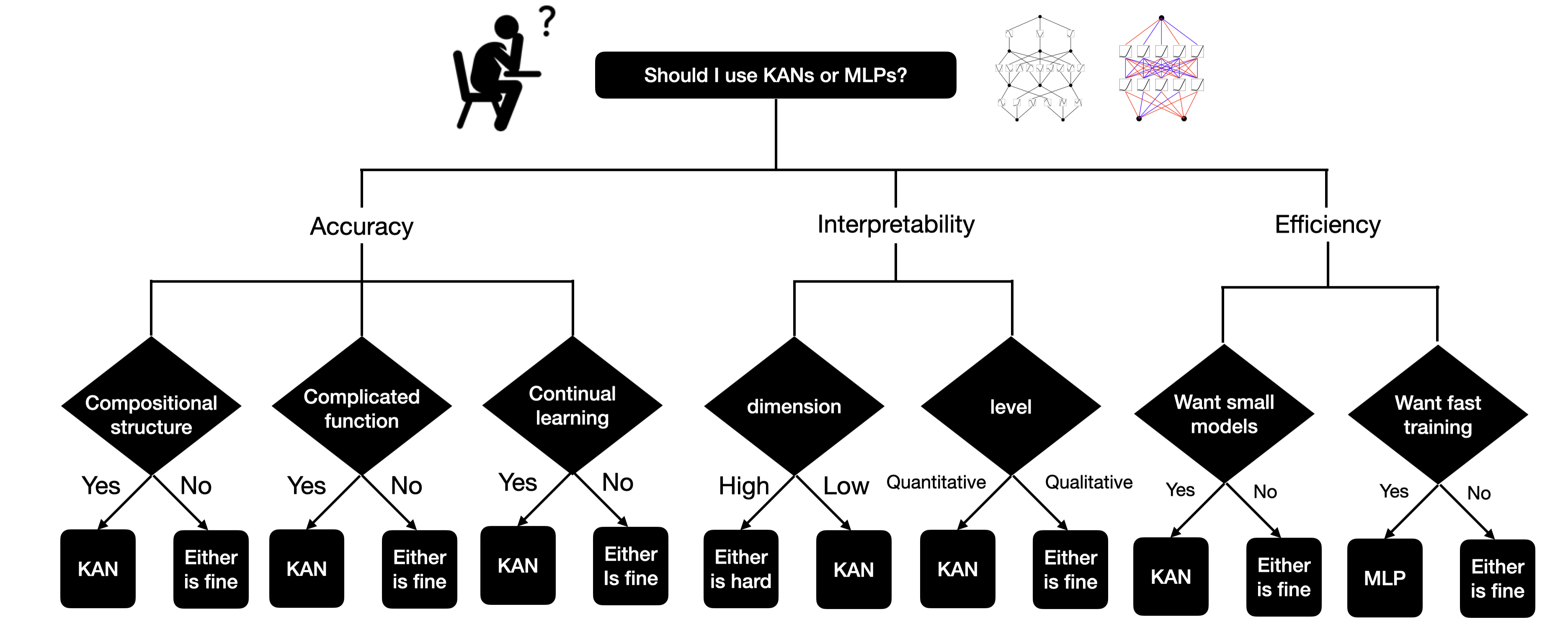
Acknowledgement

Section Summary: The authors express gratitude to numerous colleagues and researchers, including Mikail Khona, Tomaso Poggio, and others from various labs, for their helpful discussions and suggestions. Several team members receive funding from the National Science Foundation through grants like PHY-2019786 for IAIFI support, PHY-2210333 and Northeastern University startup funds for one researcher, and DMS-2205590 plus the Choi Family Gift Fund for two others. Additionally, two contributors acknowledge backing from the U.S. Office of Naval Research via a Multidisciplinary University Research Initiative grant focused on advanced photonic materials.

We would like to thank Mikail Khona, Tomaso Poggio, Pingchuan Ma, Rui Wang, Di Luo, Sara Beery, Catherine Liang, Yiping Lu, Nicholas H. Nelsen, Nikola Kovachki, Jonathan W. Siegel, Hongkai Zhao, Juncai He, Shi Lab (Humphrey Shi, Steven Walton, Chuanhao Yan) and Matthieu Darcy for fruitful discussion and constructive suggestions. Z.L., F.R., J.H., M.S. and M.T. are supported by IAIFI through NSF grant PHY-2019786. The work of FR is in addition supported by the NSF grant PHY-2210333 and by startup funding from Northeastern University. Y.W and T.H are supported by the NSF Grant DMS-2205590 and the Choi Family Gift Fund. S. V. and M. S. acknowledge support from the U.S. Office of Naval Research (ONR) Multidisciplinary University Research Initiative (MURI) under Grant No. N00014-20-1-2325 on Robust Photonic Materials with Higher-Order Topological Protection.

Appendix

Section Summary: The appendix explores learnable activation networks (LANs), which are similar to standard multilayer perceptrons but with trainable activation functions placed on nodes, making them simpler and more scalable than Kolmogorov-Arnold networks (KANs) while adding only a small number of extra parameters. However, LANs prove less interpretable and accurate than KANs due to complex weight matrices, though they can be fine-tuned from pretrained models and outperform traditional networks in tasks like image fitting by adapting activations like those in SIREN for better quality. It also discusses how hyperparameters, such as entropy penalties and grid sizes, influence the interpretability of these networks in toy examples by controlling sparsity and function expressiveness.

Appendix

A. KAN Functionalities

Table 6 includes common functionalities that users may find useful.

::: {caption="Table 6: KAN functionalities"}

:::

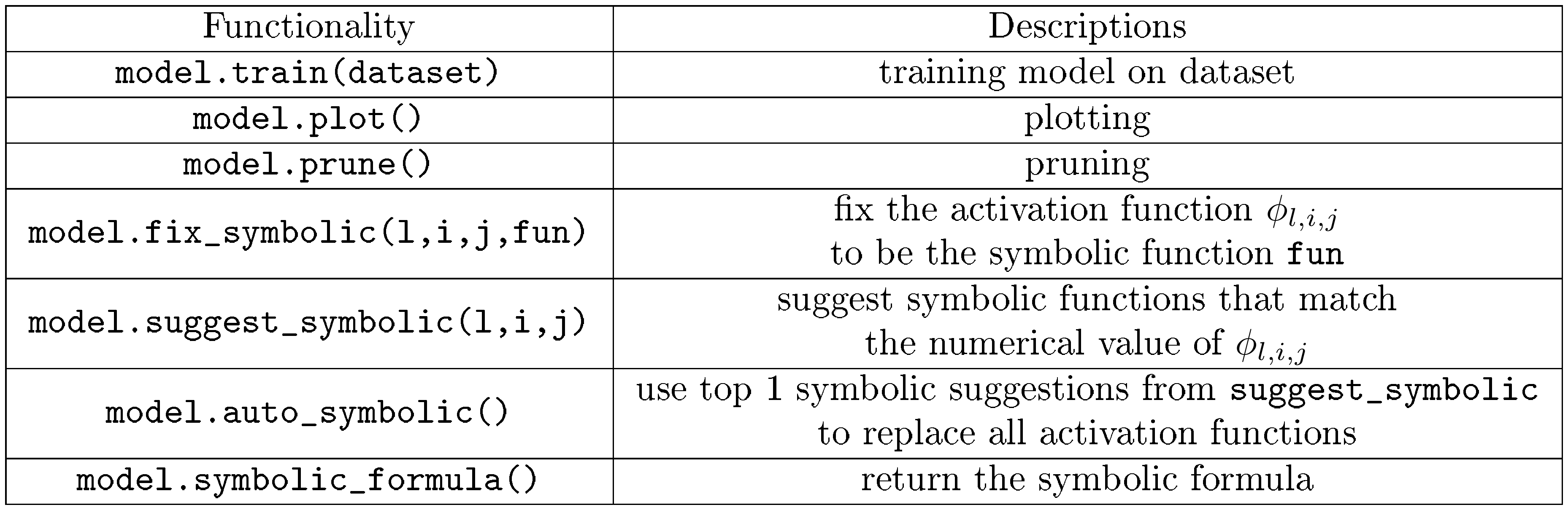
B. Learnable activation networks (LANs)

B.1 Architecture

Besides KAN, we also proposed another type of learnable activation networks (LAN), which are almost MLPs but with learnable activation functions parametrized as splines. KANs have two main changes to standard MLPs: (1) the activation functions become learnable rather than being fixed; (2) the activation functions are placed on edges rather than nodes. To disentangle these two factors, we also propose learnable activation networks (LAN) which only has learnable activations but still on nodes, illustrated in Figure 17.

For a LAN with width $N$, depth $L$, and grid point number $G$, the number of parameters is $N^2L+NLG$ where $N^2L$ is the number of parameters for weight matrices and $NLG$ is the number of parameters for spline activations, which causes little overhead in addition to MLP since usually $G\ll N$ so $NLG\ll N^2 L$. LANs are similar to MLPs so they can be initialized from pretrained MLPs and fine-tuned by allowing learnable activation functions. An example is to use LAN to improve SIREN, presented in Appendix B.3.

Comparison of LAN and KAN. Pros of LANs:

• (1) LANs are conceptually simpler than KANs. They are closer to standard MLPs (the only change is that activation functions become learnable).
• (2) LANs scale better than KANs. LANs/KANs have learnable activation functions on nodes/edges, respectively. So activation parameters in LANs/KANs scale as $N$ / $N^2$, where $N$ is model width.

Cons of LANs:

• (1) LANs seem to be less interpretable (weight matrices are hard to interpret, just like in MLPs);
• (2) LANs also seem to be less accurate than KANs, but still more accurate than MLPs. Like KANs, LANs also admit grid extension if theLANs' activation functions are parametrized by splines.

B.2 LAN interpretability results

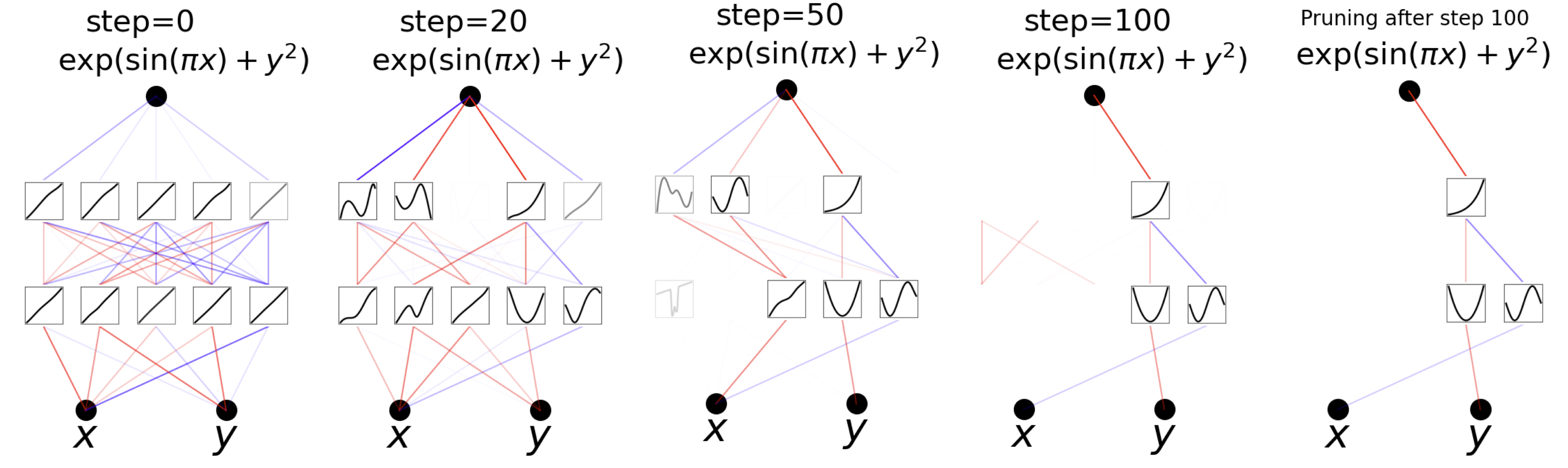
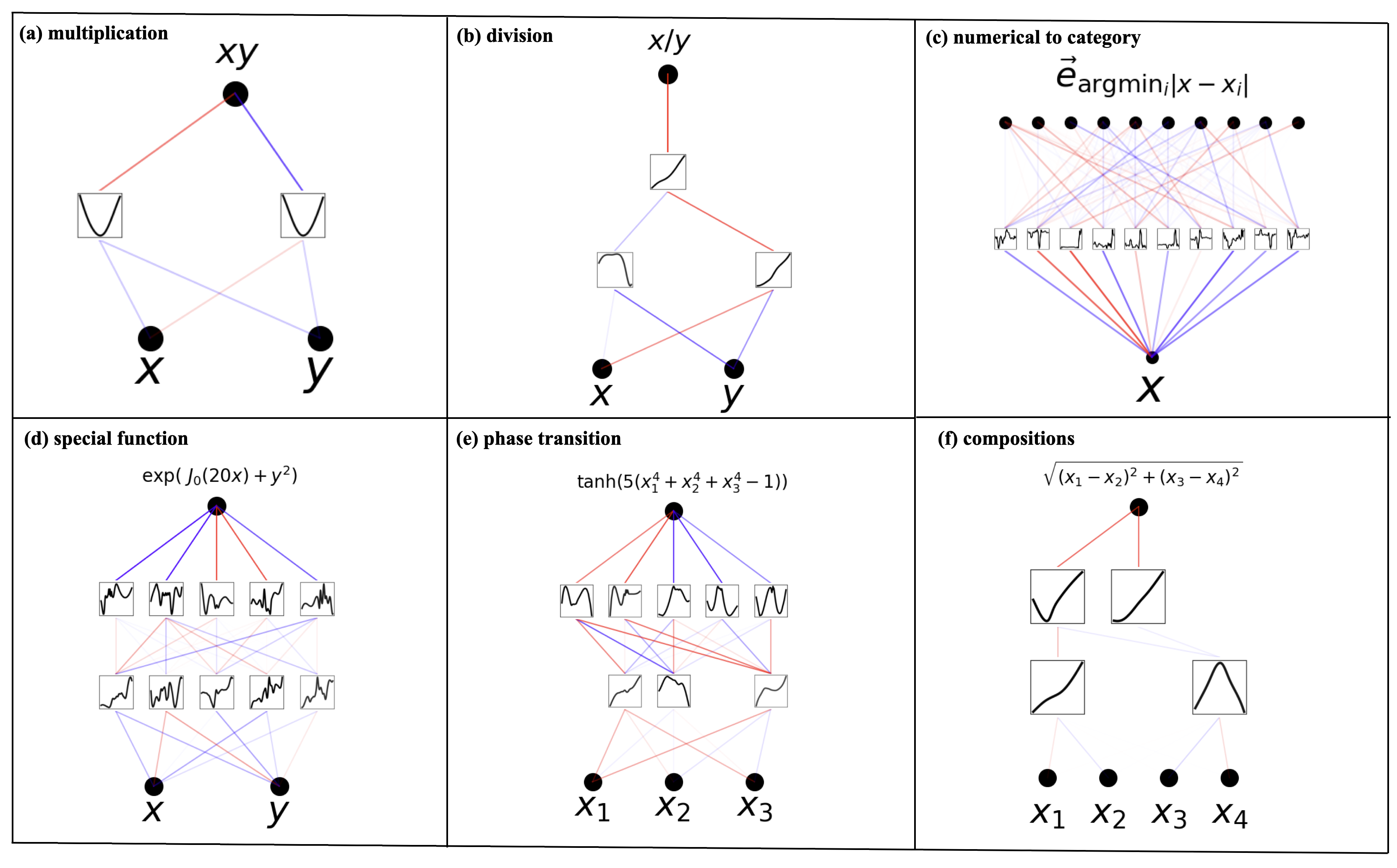
We present preliminary interpretabilty results of LANs in Figure 18. With the same examples in Figure 10 for which KANs are perfectly interpretable, LANs seem much less interpretable due to the existence of weight matrices. First, weight matrices are less readily interpretable than learnable activation functions. Second, weight matrices bring in too many degrees of freedom, making learnable activation functions too unconstrained. Our preliminary results with LANs seem to imply that getting rid of linear weight matrices (by having learnable activations on edges, like KANs) is necessary for interpretability.

B.3 Fitting Images (LAN)

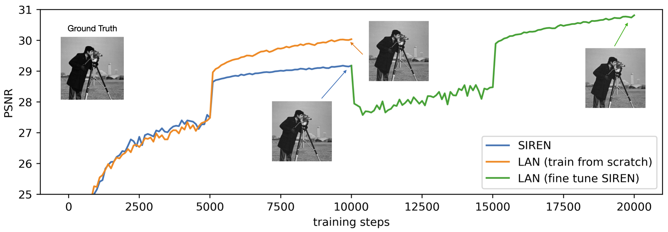
Implicit neural representations view images as 2D functions $f(x, y)$, where the pixel value $f$ is a function of two coordinates of the pixel $x$ and $y$. To compress an image, such an implicit neural representation ($f$ is a neural network) can achieve impressive compression of parameters while maintaining almost original image quality. SIREN [118] proposed to use MLPs with periodic activation functions to fit the function $f$. It is natural to consider other activation functions, which are allowed in LANs. However, since we initialize LAN activations to be smooth but SIREN requires high-frequency features, LAN does not work immediately. Note that each activation function in LANs is a sum of the base function and the spline function, i.e., $\phi(x)=b(x)+{\rm spline}(x)$, we set $b(x)$ to sine functions, the same setup as in SIREN but let ${\rm spline}(x)$ be trainable. For both MLP and LAN, the shape is [2, 128, 128, 128, 128, 128, 1]. We train them with the Adam optimizer, batch size 4096, for 5000 steps with learning rate $10^{-3}$ and 5000 steps with learning rate $10^{-4}$. As shown in Figure 19, the LAN (orange) can achieve higher PSNR than the MLP (blue) due to the LAN's flexibility to fine tune activation functions. We show that it is also possible to initialize a LAN from an MLP and further fine tune the LAN (green) for better PSNR. We have chosen $G=5$ in our experiments, so the additional parameter increase is roughly $G/N=5/128\approx 4%$ over the original parameters.

C. Dependence on hyperparameters

We show the effects of hyperparamters on the $f(x, y)={\rm exp}({\rm sin}(\pi x)+y^2)$ case in Figure 20. To get an interpretable graph, we want the number of active activation functions to be as small (ideally 3) as possible.

• (1) We need entropy penalty to reduce the number of active activation functions. Without entropy penalty, there are many duplicate functions.
• (2) Results can depend on random seeds. With some unlucky seed, the pruned network could be larger than needed.
• (3) The overall penalty strength $\lambda$ effectively controls the sparsity.
• (4) The grid number $G$ also has a subtle effect on interpretability. When $G$ is too small, because each one of activation function is not very expressive, the network tends to use the ensembling strategy, making interpretation harder.
• (5) The piecewise polynomial order $k$ only has a subtle effect on interpretability. However, it behaves a bit like the random seeds which do not display any visible pattern in this toy example.

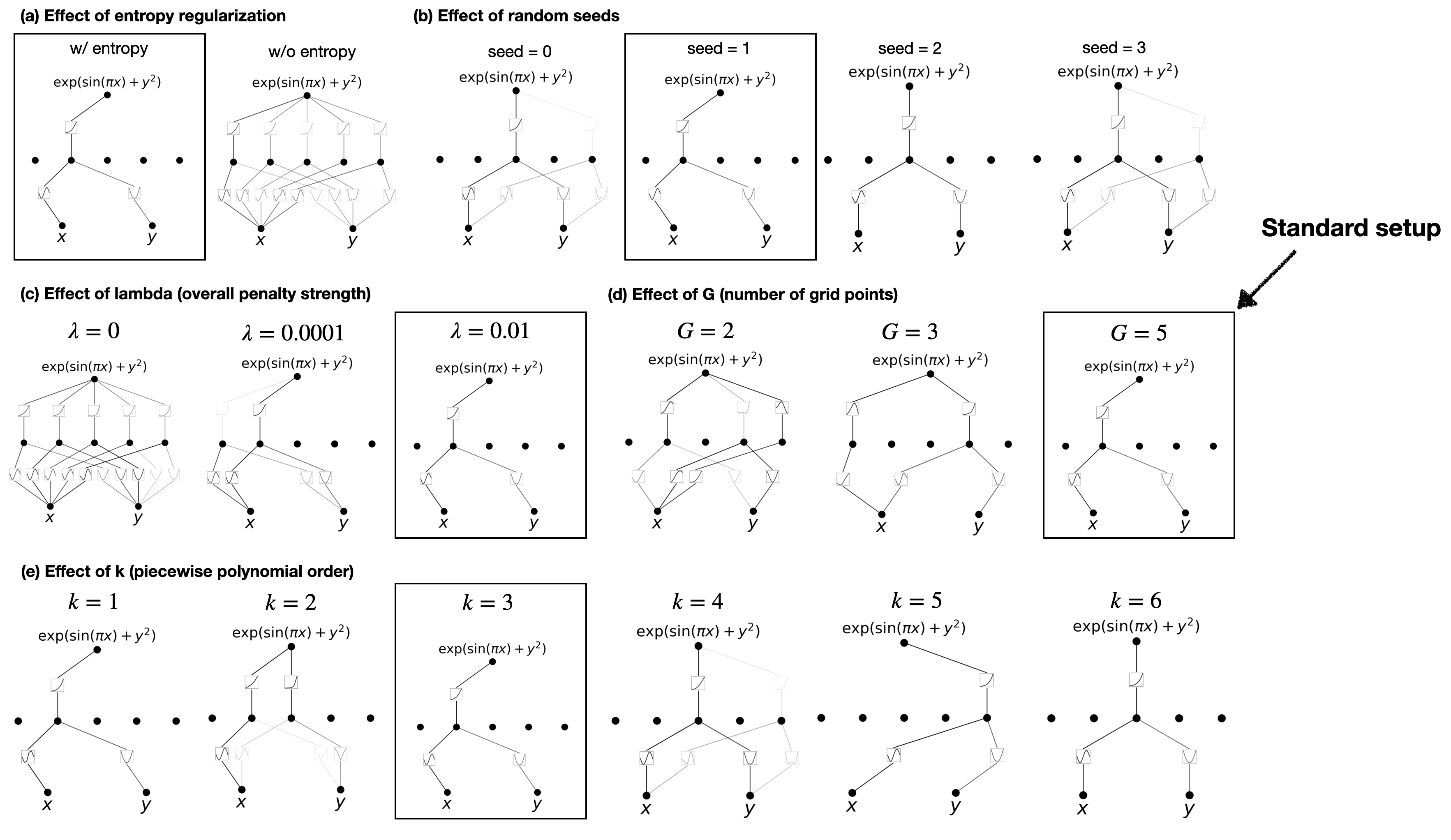
D. Feynman KANs

We include more results on the Feynman dataset (Section 3.3). Figure 21 shows the pareto frontiers of KANs and MLPs for each Feynman dataset. Figure 23 and Figure 22 visualize minimal KANs (under the constraint test RMSE

lt;10^{-2}$) and best KANs (with the lowest test RMSE loss) for each Feynman equation fitting task.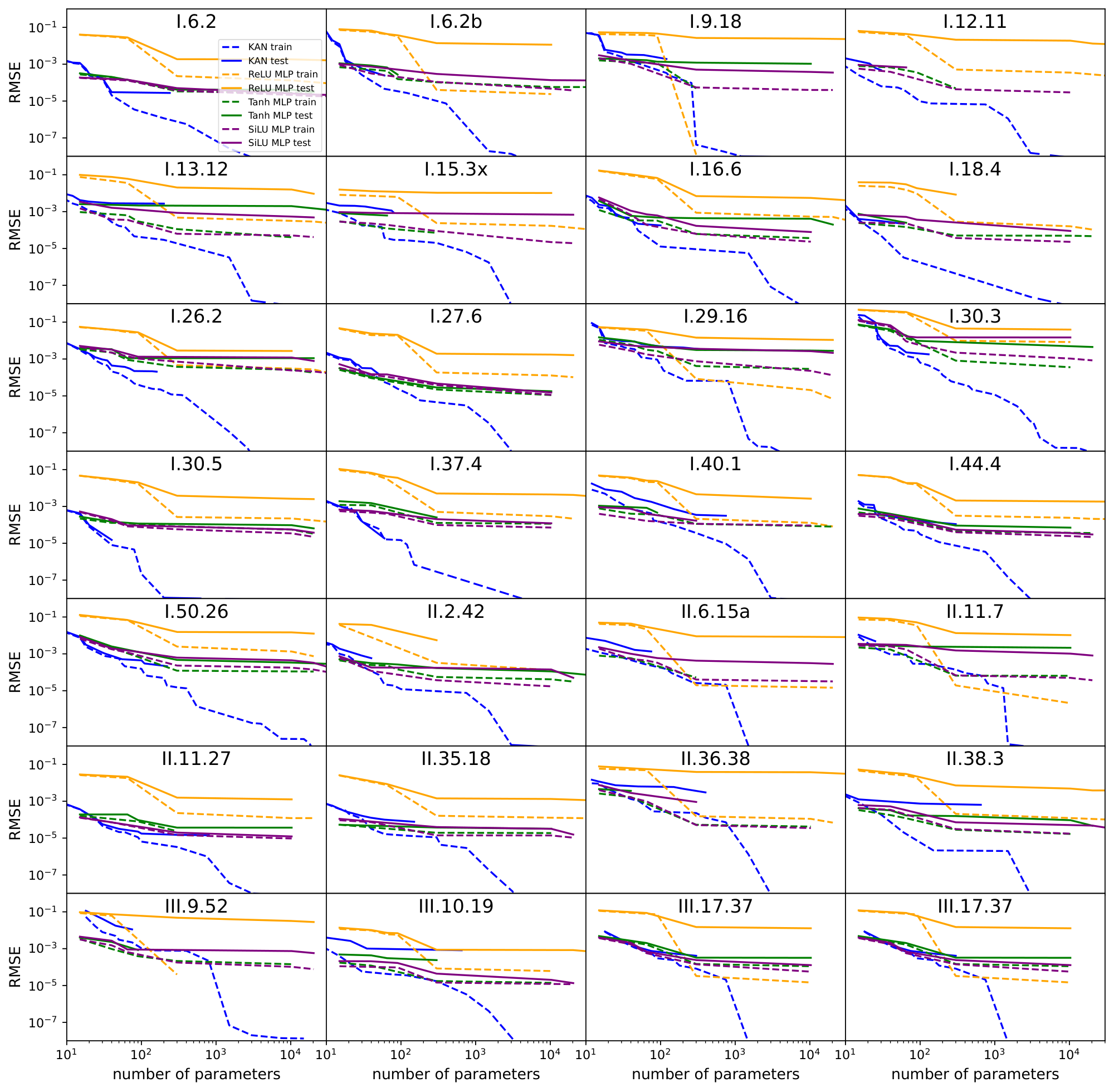

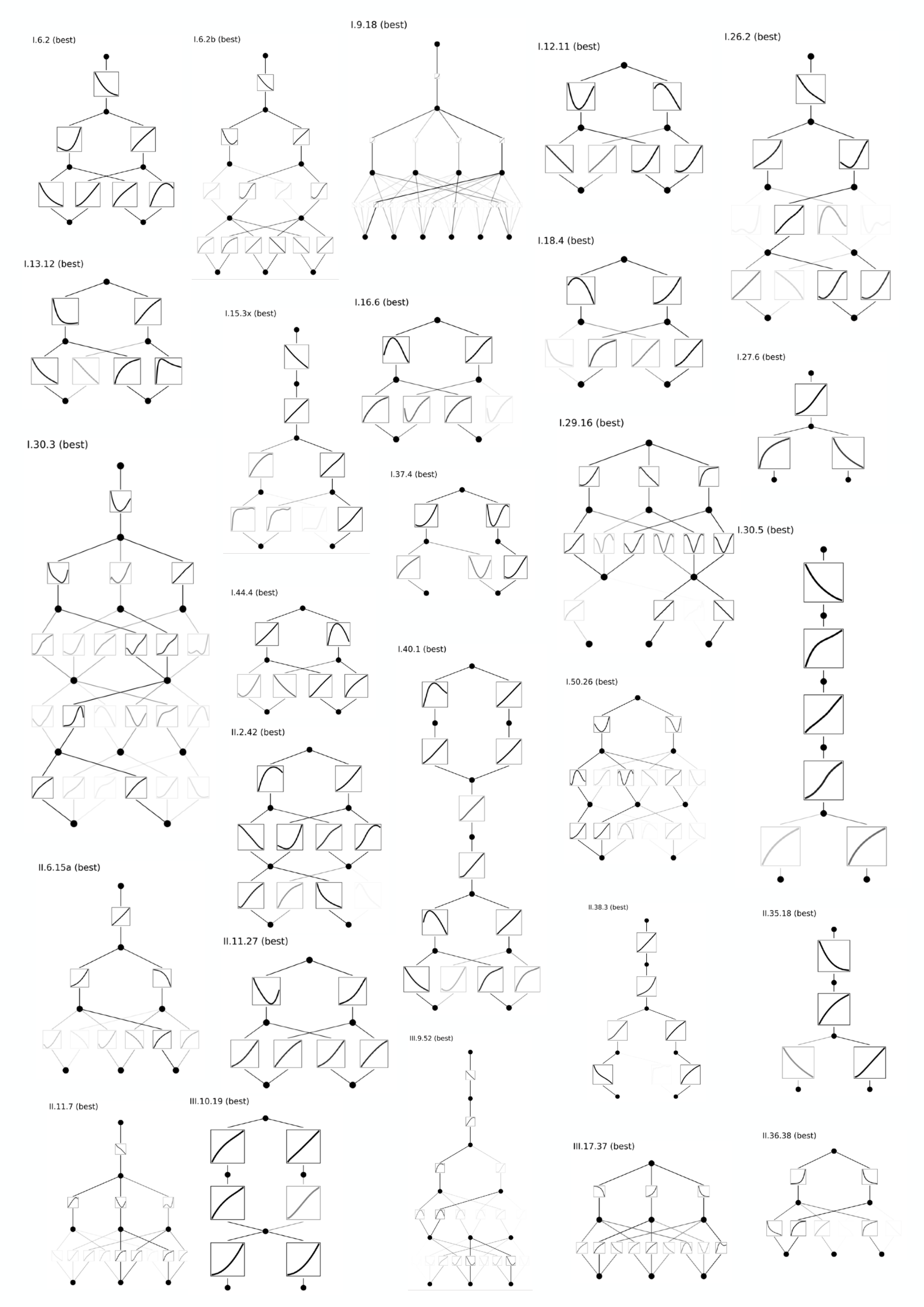
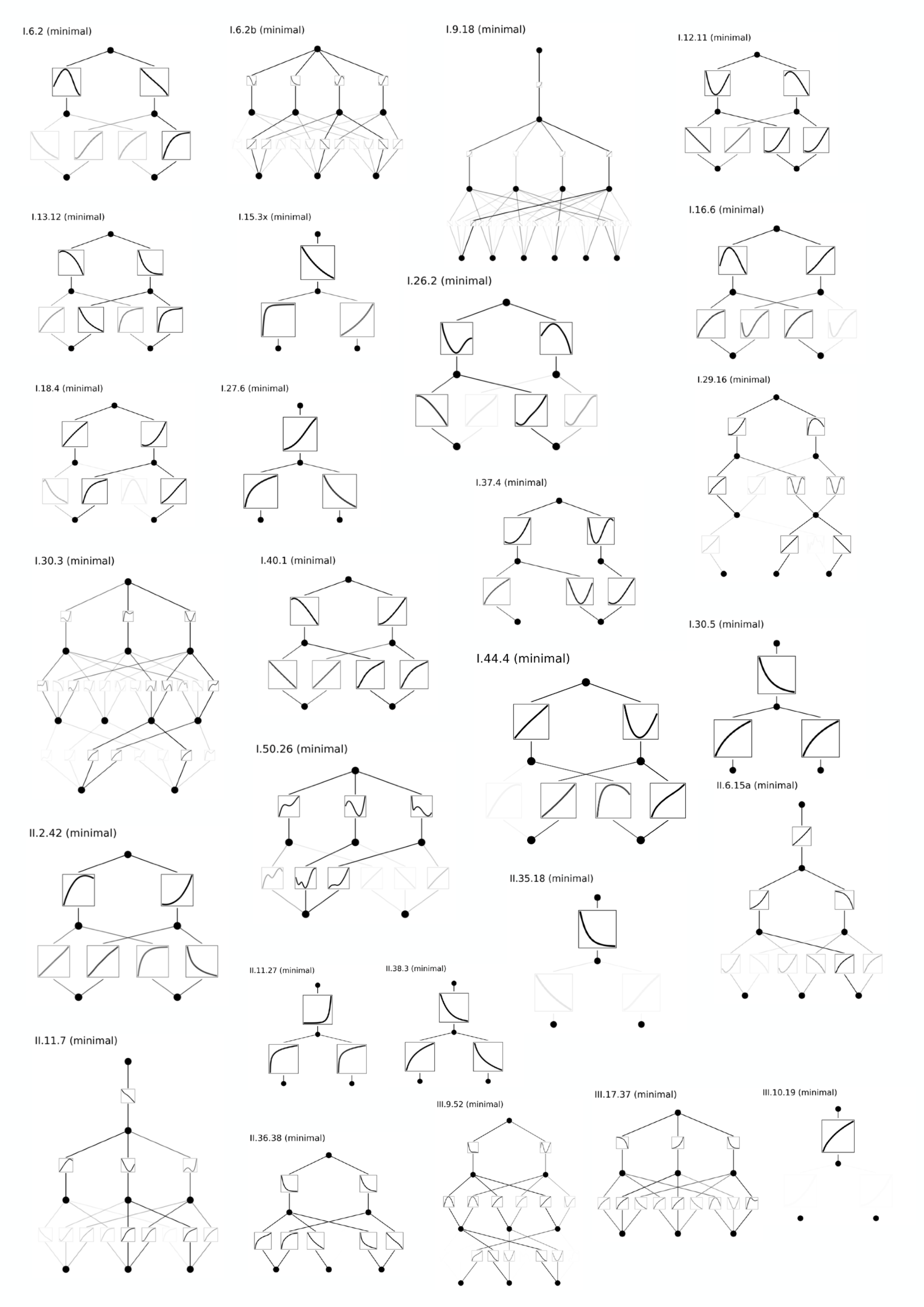
E. Remark on grid size

For both PDE and regression tasks, when we choose the training data on uniform grids, we witness a sudden increase in training loss (i.e., sudden drop in performance) when the grid size is updated to a large level, comparable to the different training points in one spatial direction. This could be due to implementation of B-spline in higher dimensions and needs further investigation.

F. KANs for special functions

We include more results on the special function dataset (Section 3.2). Figure 25 and Figure 24 visualize minimal KANs (under the constraint test RMSE

lt;10^{-2}$) and best KANs (with the lowest test RMSE loss) for each special function fitting task.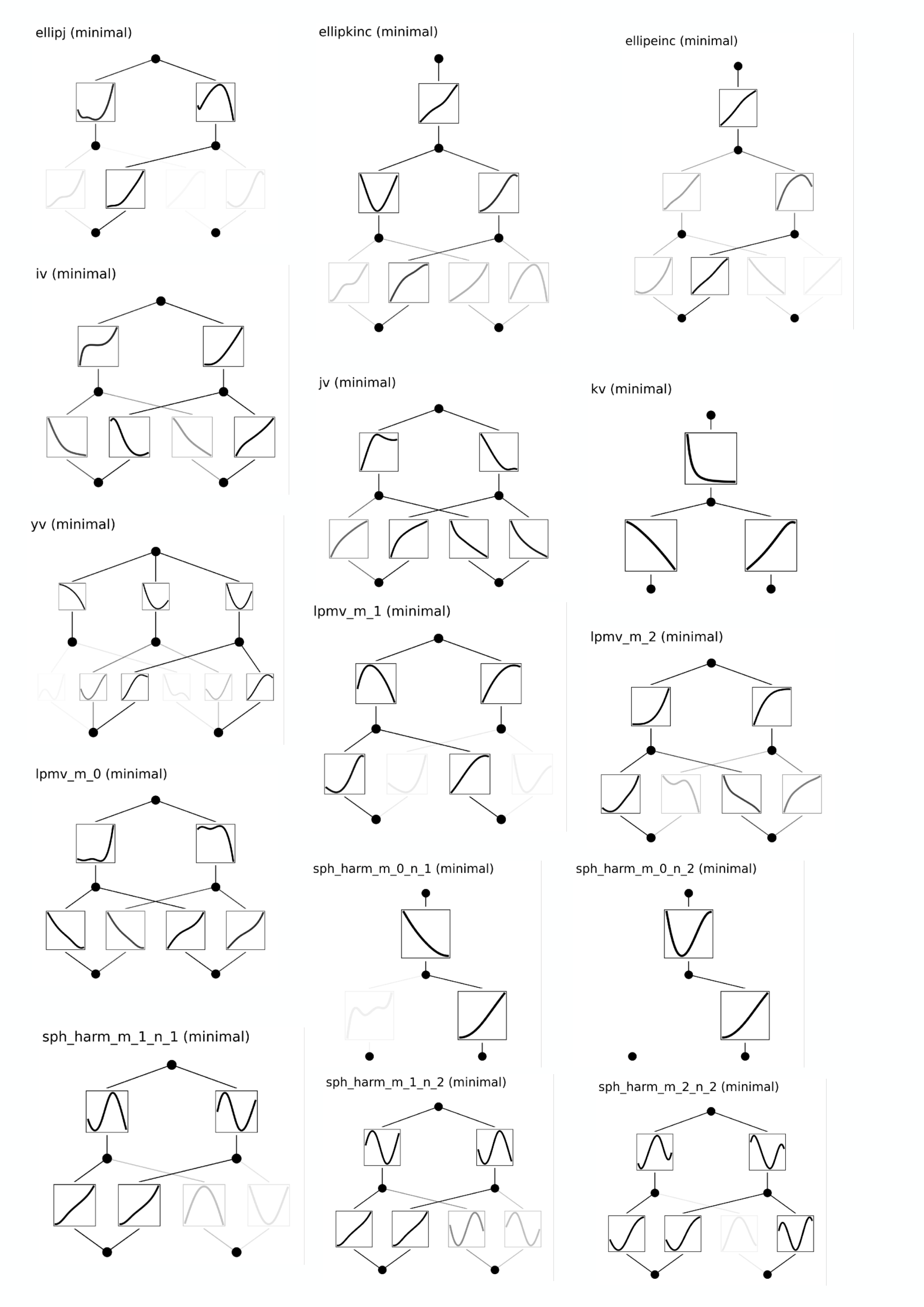

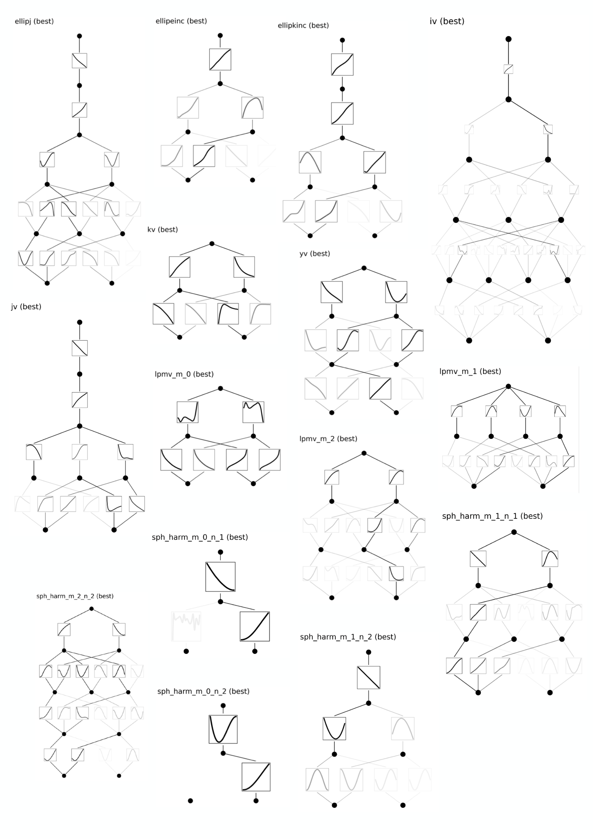
References

[1] Simon Haykin. Neural networks: a comprehensive foundation. Prentice Hall PTR, 1994.

[2] George Cybenko. Approximation by superpositions of a sigmoidal function. Mathematics of control, signals and systems, 2(4):303–314, 1989.

[3] Kurt Hornik, Maxwell Stinchcombe, and Halbert White. Multilayer feedforward networks are universal approximators. Neural networks, 2(5):359–366, 1989.

[4] Ashish Vaswani, Noam Shazeer, Niki Parmar, Jakob Uszkoreit, Llion Jones, Aidan N Gomez, Łukasz Kaiser, and Illia Polosukhin. Attention is all you need. Advances in neural information processing systems, 30, 2017.

[5] Hoagy Cunningham, Aidan Ewart, Logan Riggs, Robert Huben, and Lee Sharkey. Sparse autoencoders find highly interpretable features in language models. arXiv preprint arXiv:2309.08600, 2023.

[6] A.N. Kolmogorov. On the representation of continuous functions of several variables as superpositions of continuous functions of a smaller number of variables. Dokl. Akad. Nauk, 108(2), 1956.

[7] Andrei Nikolaevich Kolmogorov. On the representation of continuous functions of many variables by superposition of continuous functions of one variable and addition. In Doklady Akademii Nauk, volume 114, pages 953–956. Russian Academy of Sciences, 1957.

[8] Jürgen Braun and Michael Griebel. On a constructive proof of kolmogorov’s superposition theorem. Constructive approximation, 30:653–675, 2009.

[9] David A Sprecher and Sorin Draghici. Space-filling curves and kolmogorov superposition-based neural networks. Neural Networks, 15(1):57–67, 2002.

[10] Mario Köppen. On the training of a kolmogorov network. In Artificial Neural Networks—ICANN 2002: International Conference Madrid, Spain, August 28–30, 2002 Proceedings 12, pages 474–479. Springer, 2002.

[11] Ji-Nan Lin and Rolf Unbehauen. On the realization of a kolmogorov network. Neural Computation, 5(1):18–20, 1993.

[12] Ming-Jun Lai and Zhaiming Shen. The kolmogorov superposition theorem can break the curse of dimensionality when approximating high dimensional functions. arXiv preprint arXiv:2112.09963, 2021.

[13] Pierre-Emmanuel Leni, Yohan D Fougerolle, and Frédéric Truchetet. The kolmogorov spline network for image processing. In Image Processing: Concepts, Methodologies, Tools, and Applications, pages 54–78. IGI Global, 2013.

[14] Daniele Fakhoury, Emanuele Fakhoury, and Hendrik Speleers. Exsplinet: An interpretable and expressive spline-based neural network. Neural Networks, 152:332–346, 2022.

[15] Hadrien Montanelli and Haizhao Yang. Error bounds for deep relu networks using the kolmogorov–arnold superposition theorem. Neural Networks, 129:1–6, 2020.

[16] Juncai He. On the optimal expressive power of relu dnns and its application in approximation with kolmogorov superposition theorem. arXiv preprint arXiv:2308.05509, 2023.

[17] Juncai He, Lin Li, Jinchao Xu, and Chunyue Zheng. Relu deep neural networks and linear finite elements. arXiv preprint arXiv:1807.03973, 2018.

[18] Juncai He and Jinchao Xu. Deep neural networks and finite elements of any order on arbitrary dimensions. arXiv preprint arXiv:2312.14276, 2023.

[19] Tomaso Poggio, Andrzej Banburski, and Qianli Liao. Theoretical issues in deep networks. Proceedings of the National Academy of Sciences, 117(48):30039–30045, 2020.

[20] Federico Girosi and Tomaso Poggio. Representation properties of networks: Kolmogorov's theorem is irrelevant. Neural Computation, 1(4):465–469, 1989.

[21] Henry W Lin, Max Tegmark, and David Rolnick. Why does deep and cheap learning work so well? Journal of Statistical Physics, 168:1223–1247, 2017.

[22] Hongyi Xu, Funshing Sin, Yufeng Zhu, and Jernej Barbič. Nonlinear material design using principal stretches. ACM Transactions on Graphics (TOG), 34(4):1–11, 2015.

[23] Carl De Boor. A practical guide to splines, volume 27. springer-verlag New York, 1978.

[24] Utkarsh Sharma and Jared Kaplan. A neural scaling law from the dimension of the data manifold. arXiv preprint arXiv:2004.10802, 2020.

[25] Eric J Michaud, Ziming Liu, and Max Tegmark. Precision machine learning. Entropy, 25(1):175, 2023.

[26] Joel L Horowitz and Enno Mammen. Rate-optimal estimation for a general class of nonparametric regression models with unknown link functions. 2007.

[27] Michael Kohler and Sophie Langer. On the rate of convergence of fully connected deep neural network regression estimates. The Annals of Statistics, 49(4):2231–2249, 2021.

[28] Johannes Schmidt-Hieber. Nonparametric regression using deep neural networks with relu activation function. 2020.

[29] Ronald A DeVore, Ralph Howard, and Charles Micchelli. Optimal nonlinear approximation. Manuscripta mathematica, 63:469–478, 1989.

[30] Ronald A DeVore, George Kyriazis, Dany Leviatan, and Vladimir M Tikhomirov. Wavelet compression and nonlinear n-widths. Adv. Comput. Math., 1(2):197–214, 1993.

[31] Jonathan W Siegel. Sharp lower bounds on the manifold widths of sobolev and besov spaces. arXiv preprint arXiv:2402.04407, 2024.

[32] Dmitry Yarotsky. Error bounds for approximations with deep relu networks. Neural Networks, 94:103–114, 2017.

[33] Peter L Bartlett, Nick Harvey, Christopher Liaw, and Abbas Mehrabian. Nearly-tight vc-dimension and pseudodimension bounds for piecewise linear neural networks. Journal of Machine Learning Research, 20(63):1–17, 2019.

[34] Jonathan W Siegel. Optimal approximation rates for deep relu neural networks on sobolev and besov spaces. Journal of Machine Learning Research, 24(357):1–52, 2023.

[35] Yongji Wang and Ching-Yao Lai. Multi-stage neural networks: Function approximator of machine precision. Journal of Computational Physics, page 112865, 2024.

[36] Silviu-Marian Udrescu and Max Tegmark. Ai feynman: A physics-inspired method for symbolic regression. Science Advances, 6(16):eaay2631, 2020.

[37] Silviu-Marian Udrescu, Andrew Tan, Jiahai Feng, Orisvaldo Neto, Tailin Wu, and Max Tegmark. Ai feynman 2.0: Pareto-optimal symbolic regression exploiting graph modularity. Advances in Neural Information Processing Systems, 33:4860–4871, 2020.

[38] Maziar Raissi, Paris Perdikaris, and George E Karniadakis. Physics-informed neural networks: A deep learning framework for solving forward and inverse problems involving nonlinear partial differential equations. Journal of Computational physics, 378:686–707, 2019.

[39] George Em Karniadakis, Ioannis G Kevrekidis, Lu Lu, Paris Perdikaris, Sifan Wang, and Liu Yang. Physics-informed machine learning. Nature Reviews Physics, 3(6):422–440, 2021.

[40] Ronald Kemker, Marc McClure, Angelina Abitino, Tyler Hayes, and Christopher Kanan. Measuring catastrophic forgetting in neural networks. In Proceedings of the AAAI conference on artificial intelligence, volume 32, 2018.

[41] Bryan Kolb and Ian Q Whishaw. Brain plasticity and behavior. Annual review of psychology, 49(1):43–64, 1998.

[42] David Meunier, Renaud Lambiotte, and Edward T Bullmore. Modular and hierarchically modular organization of brain networks. Frontiers in neuroscience, 4:7572, 2010.

[43] James Kirkpatrick, Razvan Pascanu, Neil Rabinowitz, Joel Veness, Guillaume Desjardins, Andrei A Rusu, Kieran Milan, John Quan, Tiago Ramalho, Agnieszka Grabska-Barwinska, et al. Overcoming catastrophic forgetting in neural networks. Proceedings of the national academy of sciences, 114(13):3521–3526, 2017.

[44] Aojun Lu, Tao Feng, Hangjie Yuan, Xiaotian Song, and Yanan Sun. Revisiting neural networks for continual learning: An architectural perspective, 2024.

[45] Alex Davies, Petar Veličković, Lars Buesing, Sam Blackwell, Daniel Zheng, Nenad Tomašev, Richard Tanburn, Peter Battaglia, Charles Blundell, András Juhász, et al. Advancing mathematics by guiding human intuition with ai. Nature, 600(7887):70–74, 2021.

[46] Sergei Gukov, James Halverson, Ciprian Manolescu, and Fabian Ruehle. Searching for ribbons with machine learning, 2023.

[47] P. Petersen. Riemannian Geometry. Graduate Texts in Mathematics. Springer New York, 2006.

[48] Philip W Anderson. Absence of diffusion in certain random lattices. Physical review, 109(5):1492, 1958.

[49] David J Thouless. A relation between the density of states and range of localization for one dimensional random systems. Journal of Physics C: Solid State Physics, 5(1):77, 1972.

[50] Elihu Abrahams, PW Anderson, DC Licciardello, and TV Ramakrishnan. Scaling theory of localization: Absence of quantum diffusion in two dimensions. Physical Review Letters, 42(10):673, 1979.

[51] Ad Lagendijk, Bart van Tiggelen, and Diederik S Wiersma. Fifty years of anderson localization. Physics today, 62(8):24–29, 2009.

[52] Mordechai Segev, Yaron Silberberg, and Demetrios N Christodoulides. Anderson localization of light. Nature Photonics, 7(3):197–204, 2013.

[53] Z Valy Vardeny, Ajay Nahata, and Amit Agrawal. Optics of photonic quasicrystals. Nature photonics, 7(3):177–187, 2013.

[54] Sajeev John. Strong localization of photons in certain disordered dielectric superlattices. Physical review letters, 58(23):2486, 1987.

[55] Yoav Lahini, Rami Pugatch, Francesca Pozzi, Marc Sorel, Roberto Morandotti, Nir Davidson, and Yaron Silberberg. Observation of a localization transition in quasiperiodic photonic lattices. Physical review letters, 103(1):013901, 2009.

[56] Sachin Vaidya, Christina Jörg, Kyle Linn, Megan Goh, and Mikael C Rechtsman. Reentrant delocalization transition in one-dimensional photonic quasicrystals. Physical Review Research, 5(3):033170, 2023.

[57] Wojciech De Roeck, Francois Huveneers, Markus Müller, and Mauro Schiulaz. Absence of many-body mobility edges. Physical Review B, 93(1):014203, 2016.

[58] Xiaopeng Li, Sriram Ganeshan, JH Pixley, and S Das Sarma. Many-body localization and quantum nonergodicity in a model with a single-particle mobility edge. Physical review letters, 115(18):186601, 2015.

[59] Fangzhao Alex An, Karmela Padavić, Eric J Meier, Suraj Hegde, Sriram Ganeshan, JH Pixley, Smitha Vishveshwara, and Bryce Gadway. Interactions and mobility edges: Observing the generalized aubry-andré model. Physical review letters, 126(4):040603, 2021.

[60] J Biddle and S Das Sarma. Predicted mobility edges in one-dimensional incommensurate optical lattices: An exactly solvable model of anderson localization. Physical review letters, 104(7):070601, 2010.

[61] Alexander Duthie, Sthitadhi Roy, and David E Logan. Self-consistent theory of mobility edges in quasiperiodic chains. Physical Review B, 103(6):L060201, 2021.

[62] Sriram Ganeshan, JH Pixley, and S Das Sarma. Nearest neighbor tight binding models with an exact mobility edge in one dimension. Physical review letters, 114(14):146601, 2015.

[63] Yucheng Wang, Xu Xia, Long Zhang, Hepeng Yao, Shu Chen, Jiangong You, Qi Zhou, and Xiong-Jun Liu. One-dimensional quasiperiodic mosaic lattice with exact mobility edges. Physical Review Letters, 125(19):196604, 2020.

[64] Yucheng Wang, Xu Xia, Yongjian Wang, Zuohuan Zheng, and Xiong-Jun Liu. Duality between two generalized aubry-andré models with exact mobility edges. Physical Review B, 103(17):174205, 2021.

[65] Xin-Chi Zhou, Yongjian Wang, Ting-Fung Jeffrey Poon, Qi Zhou, and Xiong-Jun Liu. Exact new mobility edges between critical and localized states. Physical Review Letters, 131(17):176401, 2023.

[66] Tomaso Poggio. How deep sparse networks avoid the curse of dimensionality: Efficiently computable functions are compositionally sparse. CBMM Memo, 10:2022, 2022.

[67] Johannes Schmidt-Hieber. The kolmogorov–arnold representation theorem revisited. Neural networks, 137:119–126, 2021.

[68] Aysu Ismayilova and Vugar E Ismailov. On the kolmogorov neural networks. Neural Networks, page 106333, 2024.

[69] Michael Poluektov and Andrew Polar. A new iterative method for construction of the kolmogorov-arnold representation. arXiv preprint arXiv:2305.08194, 2023.

[70] Rishabh Agarwal, Levi Melnick, Nicholas Frosst, Xuezhou Zhang, Ben Lengerich, Rich Caruana, and Geoffrey E Hinton. Neural additive models: Interpretable machine learning with neural nets. Advances in neural information processing systems, 34:4699–4711, 2021.

[71] Manzil Zaheer, Satwik Kottur, Siamak Ravanbakhsh, Barnabas Poczos, Russ R Salakhutdinov, and Alexander J Smola. Deep sets. Advances in neural information processing systems, 30, 2017.

[72] Huan Song, Jayaraman J Thiagarajan, Prasanna Sattigeri, and Andreas Spanias. Optimizing kernel machines using deep learning. IEEE transactions on neural networks and learning systems, 29(11):5528–5540, 2018.

[73] Jared Kaplan, Sam McCandlish, Tom Henighan, Tom B Brown, Benjamin Chess, Rewon Child, Scott Gray, Alec Radford, Jeffrey Wu, and Dario Amodei. Scaling laws for neural language models. arXiv preprint arXiv:2001.08361, 2020.

[74] Tom Henighan, Jared Kaplan, Mor Katz, Mark Chen, Christopher Hesse, Jacob Jackson, Heewoo Jun, Tom B Brown, Prafulla Dhariwal, Scott Gray, et al. Scaling laws for autoregressive generative modeling. arXiv preprint arXiv:2010.14701, 2020.

[75] Mitchell A Gordon, Kevin Duh, and Jared Kaplan. Data and parameter scaling laws for neural machine translation. In ACL Rolling Review - May 2021, 2021.

[76] Joel Hestness, Sharan Narang, Newsha Ardalani, Gregory Diamos, Heewoo Jun, Hassan Kianinejad, Md Mostofa Ali Patwary, Yang Yang, and Yanqi Zhou. Deep learning scaling is predictable, empirically. arXiv preprint arXiv:1712.00409, 2017.

[77] Yasaman Bahri, Ethan Dyer, Jared Kaplan, Jaehoon Lee, and Utkarsh Sharma. Explaining neural scaling laws. arXiv preprint arXiv:2102.06701, 2021.

[78] Eric J Michaud, Ziming Liu, Uzay Girit, and Max Tegmark. The quantization model of neural scaling. In Thirty-seventh Conference on Neural Information Processing Systems, 2023.

[79] Jinyeop Song, Ziming Liu, Max Tegmark, and Jeff Gore. A resource model for neural scaling law. arXiv preprint arXiv:2402.05164, 2024.

[80] Catherine Olsson, Nelson Elhage, Neel Nanda, Nicholas Joseph, Nova DasSarma, Tom Henighan, Ben Mann, Amanda Askell, Yuntao Bai, Anna Chen, et al. In-context learning and induction heads. arXiv preprint arXiv:2209.11895, 2022.

[81] Kevin Meng, David Bau, Alex Andonian, and Yonatan Belinkov. Locating and editing factual associations in gpt. Advances in Neural Information Processing Systems, 35:17359–17372, 2022.

[82] Kevin Ro Wang, Alexandre Variengien, Arthur Conmy, Buck Shlegeris, and Jacob Steinhardt. Interpretability in the wild: a circuit for indirect object identification in GPT-2 small. In The Eleventh International Conference on Learning Representations, 2023.

[83] Nelson Elhage, Tristan Hume, Catherine Olsson, Nicholas Schiefer, Tom Henighan, Shauna Kravec, Zac Hatfield-Dodds, Robert Lasenby, Dawn Drain, Carol Chen, et al. Toy models of superposition. arXiv preprint arXiv:2209.10652, 2022.

[84] Neel Nanda, Lawrence Chan, Tom Lieberum, Jess Smith, and Jacob Steinhardt. Progress measures for grokking via mechanistic interpretability. In The Eleventh International Conference on Learning Representations, 2023.

[85] Ziqian Zhong, Ziming Liu, Max Tegmark, and Jacob Andreas. The clock and the pizza: Two stories in mechanistic explanation of neural networks. In Thirty-seventh Conference on Neural Information Processing Systems, 2023.

[86] Ziming Liu, Eric Gan, and Max Tegmark. Seeing is believing: Brain-inspired modular training for mechanistic interpretability. Entropy, 26(1):41, 2023.

[87] Nelson Elhage, Tristan Hume, Catherine Olsson, Neel Nanda, Tom Henighan, Scott Johnston, Sheer ElShowk, Nicholas Joseph, Nova DasSarma, Ben Mann, Danny Hernandez, Amanda Askell, Kamal Ndousse, Andy Jones, Dawn Drain, Anna Chen, Yuntao Bai, Deep Ganguli, Liane Lovitt, Zac Hatfield-Dodds, Jackson Kernion, Tom Conerly, Shauna Kravec, Stanislav Fort, Saurav Kadavath, Josh Jacobson, Eli Tran-Johnson, Jared Kaplan, Jack Clark, Tom Brown, Sam McCandlish, Dario Amodei, and Christopher Olah. Softmax linear units. Transformer Circuits Thread, 2022. https://transformer-circuits.pub/2022/solu/index.html.

[88] Mohit Goyal, Rajan Goyal, and Brejesh Lall. Learning activation functions: A new paradigm for understanding neural networks. arXiv preprint arXiv:1906.09529, 2019.

[89] Prajit Ramachandran, Barret Zoph, and Quoc V Le. Searching for activation functions. arXiv preprint arXiv:1710.05941, 2017.

[90] Shijun Zhang, Zuowei Shen, and Haizhao Yang. Neural network architecture beyond width and depth. Advances in Neural Information Processing Systems, 35:5669–5681, 2022.

[91] Garrett Bingham and Risto Miikkulainen. Discovering parametric activation functions. Neural Networks, 148:48–65, 2022.

[92] Pakshal Bohra, Joaquim Campos, Harshit Gupta, Shayan Aziznejad, and Michael Unser. Learning activation functions in deep (spline) neural networks. IEEE Open Journal of Signal Processing, 1:295–309, 2020.

[93] Shayan Aziznejad and Michael Unser. Deep spline networks with control of lipschitz regularity. In ICASSP 2019-2019 IEEE International Conference on Acoustics, Speech and Signal Processing (ICASSP), pages 3242–3246. IEEE, 2019.

[94] Renáta Dubcáková. Eureqa: software review. Genetic Programming and Evolvable Machines, 12:173–178, 2011.

[95] Gplearn. https://github.com/trevorstephens/gplearn. Accessed: 2024-04-19.

[96] Miles Cranmer. Interpretable machine learning for science with pysr and symbolicregression. jl. arXiv preprint arXiv:2305.01582, 2023.

[97] Georg Martius and Christoph H Lampert. Extrapolation and learning equations. arXiv preprint arXiv:1610.02995, 2016.

[98] Owen Dugan, Rumen Dangovski, Allan Costa, Samuel Kim, Pawan Goyal, Joseph Jacobson, and Marin Soljačić. Occamnet: A fast neural model for symbolic regression at scale. arXiv preprint arXiv:2007.10784, 2020.

[99] Terrell N. Mundhenk, Mikel Landajuela, Ruben Glatt, Claudio P. Santiago, Daniel faissol, and Brenden K. Petersen. Symbolic regression via deep reinforcement learning enhanced genetic programming seeding. In A. Beygelzimer, Y. Dauphin, P. Liang, and J. Wortman Vaughan, editors, Advances in Neural Information Processing Systems, 2021.

[100] Bing Yu et al. The deep ritz method: a deep learning-based numerical algorithm for solving variational problems. Communications in Mathematics and Statistics, 6(1):1–12, 2018.

[101] Junwoo Cho, Seungtae Nam, Hyunmo Yang, Seok-Bae Yun, Youngjoon Hong, and Eunbyung Park. Separable physics-informed neural networks. Advances in Neural Information Processing Systems, 36, 2024.

[102] Zongyi Li, Nikola Kovachki, Kamyar Azizzadenesheli, Burigede Liu, Kaushik Bhattacharya, Andrew Stuart, and Anima Anandkumar. Fourier neural operator for parametric partial differential equations. arXiv preprint arXiv:2010.08895, 2020.

[103] Zongyi Li, Hongkai Zheng, Nikola Kovachki, David Jin, Haoxuan Chen, Burigede Liu, Kamyar Azizzadenesheli, and Anima Anandkumar. Physics-informed neural operator for learning partial differential equations. ACM/JMS Journal of Data Science, 2021.

[104] Nikola Kovachki, Zongyi Li, Burigede Liu, Kamyar Azizzadenesheli, Kaushik Bhattacharya, Andrew Stuart, and Anima Anandkumar. Neural operator: Learning maps between function spaces with applications to pdes. Journal of Machine Learning Research, 24(89):1–97, 2023.

[105] Haydn Maust, Zongyi Li, Yixuan Wang, Daniel Leibovici, Oscar Bruno, Thomas Hou, and Anima Anandkumar. Fourier continuation for exact derivative computation in physics-informed neural operators. arXiv preprint arXiv:2211.15960, 2022.

[106] Lu Lu, Pengzhan Jin, Guofei Pang, Zhongqiang Zhang, and George Em Karniadakis. Learning nonlinear operators via deeponet based on the universal approximation theorem of operators. Nature machine intelligence, 3(3):218–229, 2021.

[107] Sergei Gukov, James Halverson, Fabian Ruehle, and Piotr Sułkowski. Learning to Unknot. Mach. Learn. Sci. Tech., 2(2):025035, 2021.

[108] L. H. Kauffman, N. E. Russkikh, and I. A. Taimanov. Rectangular knot diagrams classification with deep learning, 2020.

[109] Mark C Hughes. A neural network approach to predicting and computing knot invariants. Journal of Knot Theory and Its Ramifications, 29(03):2050005, 2020.

[110] Jessica Craven, Vishnu Jejjala, and Arjun Kar. Disentangling a deep learned volume formula. JHEP, 06:040, 2021.

[111] Jessica Craven, Mark Hughes, Vishnu Jejjala, and Arjun Kar. Illuminating new and known relations between knot invariants. 11 2022.

[112] Fabian Ruehle. Data science applications to string theory. Phys. Rept., 839:1–117, 2020.

[113] Y.H. He. Machine Learning in Pure Mathematics and Theoretical Physics. G - Reference,Information and Interdisciplinary Subjects Series. World Scientific, 2023.

[114] Sergei Gukov, James Halverson, and Fabian Ruehle. Rigor with machine learning from field theory to the poincaréconjecture. Nature Reviews Physics, 2024.

[115] Shumao Zhang, Pengchuan Zhang, and Thomas Y Hou. Multiscale invertible generative networks for high-dimensional bayesian inference. In International Conference on Machine Learning, pages 12632–12641. PMLR, 2021.

[116] Jinchao Xu and Ludmil Zikatanov. Algebraic multigrid methods. Acta Numerica, 26:591–721, 2017.

[117] Yifan Chen, Thomas Y Hou, and Yixuan Wang. Exponentially convergent multiscale finite element method. Communications on Applied Mathematics and Computation, pages 1–17, 2023.

[118] Vincent Sitzmann, Julien Martel, Alexander Bergman, David Lindell, and Gordon Wetzstein. Implicit neural representations with periodic activation functions. Advances in neural information processing systems, 33:7462–7473, 2020.