
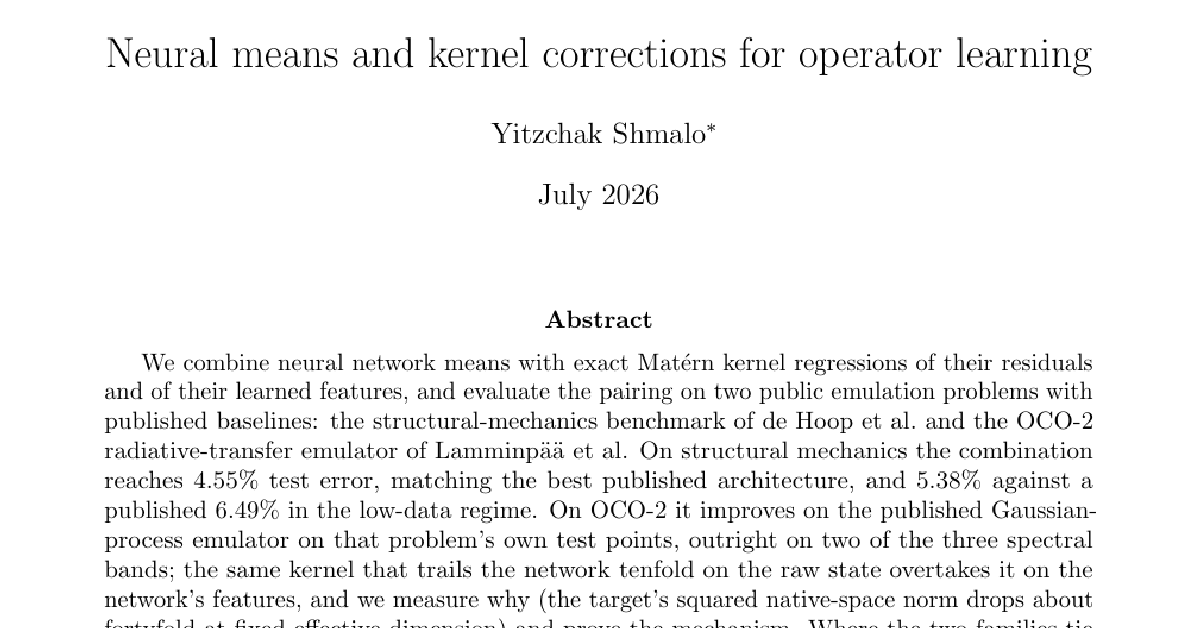
Neural means and kernel corrections for operator learning
Yitzchak Shmalo $^{*}$
$^{*}$ Einstein Institute of Mathematics, The Hebrew University of Jerusalem, Jerusalem, Israel. [email protected]. Code, data pointers, and the per-run summaries behind every number reported here are at https://github.com/yspennstate/neural-means-kernel-corrections.
Abstract
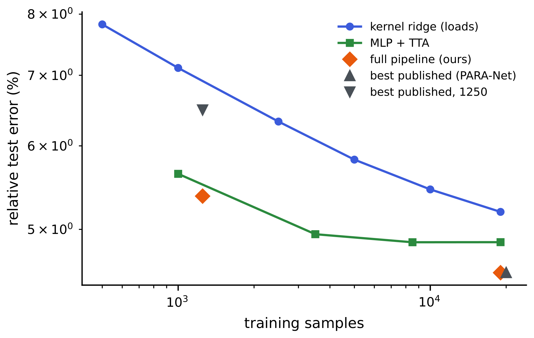
We combine neural network means with exact Matérn kernel regressions of their residuals and of their learned features, and evaluate the pairing on two public emulation problems with published baselines: the structural-mechanics benchmark of de Hoop et al.\ and the OCO-2 radiative-transfer emulator of Lamminpää et al. On structural mechanics the combination reaches 4.55% test error, matching the best published architecture, and 5.38% against a published 6.49% in the low-data regime. On OCO-2 it improves on the published Gaussian-process emulator on that problem's own test points, outright on two of the three spectral bands; the same kernel that trails the network tenfold on the raw state overtakes it on the network's features, and we measure why (the target's squared native-space norm drops about fortyfold at fixed effective dimension) and prove the mechanism. Where the two families tie instead, the residuals of every architecture we train correlate above 0.86 and their shared component is flat in diversity and sample size, which reads the published plateau as a property of the data. Supporting results include a second-moment identity that predicts stacking outcomes from measured correlations, an optimal-recovery certificate, and a distribution-free coverage band, the only uncertainty signal that survives our tests.
Executive Summary: This book presents a hybrid pipeline for operator learning that combines flexible neural network means with exact kernel ridge regression corrections. Aimed at researchers, computational scientists, and graduate students working at the intersection of scientific machine learning, numerical analysis, and surrogate modeling, the text assumes familiarity with partial differential equations, functional analysis, reproducing kernel Hilbert spaces, deep neural networks, and basic random matrix theory. It systematically addresses the challenge of building fast, highly accurate surrogates for physical forward models, defining clear boundaries between what neural networks, kernel methods, and their hybrid pairings can achieve across varying data and representation regimes.
The pedagogical progression advances from problem formulation and model architectures to empirical benchmarks, diagnostics, and foundational mathematical theory. The primary framework couples three sequential stages: training neural network means (such as residual multilayer perceptrons, kernel-conditioned refiners, UNets, and Fourier neural operators) using metric-aligned loss functions and domain symmetries; constructing convex stacked ensembles; and applying exact Matérn kernel ridge regression to the resulting residuals and learned penultimate features. The text details two operational regimes: a balanced regime where neural networks and kernel methods perform comparably, and an asymmetric regime where kernels applied directly to raw inputs trail neural representations by an order of magnitude, necessitating feature-space kernel heads and coordinate-specific metric tuning.
From a practical standpoint, the book teaches methods for identifying and exploiting problem symmetries through reflection augmentation and test-time symmetrization, diagnosing the limit of ensemble models via second-moment error correlation matrices, and computing exact kernel solves at scale without resorting to inducing-point approximations. It provides rigorous protocols for surrogate evaluation using standard operator learning suites (including structural mechanics elasticity benchmarks, OCO-2 satellite radiative transfer emulation, and ClimSim climate models). Readers also learn to implement split conformal prediction to obtain reliable distribution-free coverage bands for uncertainty quantification, overcoming the limitations of standard Gaussian process posterior variances that fail as pointwise error rankers.
After studying this book, readers will be able to design, implement, and certify hybrid operator-learning surrogates tailored to parametric scientific problems. They will understand how to diagnose whether an empirical error plateau is caused by model capacity or by data-generation noise, analyze the effective dimension of kernel Gram spectra, and mathematically predict ensemble gains. The book explicitly excludes high-dimensional spatial input approximations (such as stochastic trace estimators or inducing points for dense fields), iterative fine-tuning through end-to-end Gaussian process marginal likelihood backpropagation, and extensive solver re-generation, focusing instead on exact solves, post-hoc residual corrections, and rigorous analytical certificates.
1. Introduction
Section Summary: This paper presents a hybrid method that pairs a neural-network mean function, trained directly on application-specific error metrics, with an exact Matérn kernel regression on the network’s residuals and learned features. The resulting pipeline is evaluated on structural-mechanics and atmospheric-radiance emulation tasks as well as a seven-problem operator-learning benchmark suite, where it matches or improves upon the best published accuracies while supplying exact solves and uncertainty estimates. Supporting theory shows how the kernel stage reduces the effective target norm and yields distribution-free coverage guarantees once the design factor is recalibrated by split conformal prediction.
Operator learning constructs fast surrogates for the solution maps of parametric partial differential equations and physical forward models. Neural operators ([1, 2, 3]) learn their own representations; kernel and Gaussian-process methods ([4, 5, 6]) come with exact solves and error certificates and a strong record on the same benchmarks. This paper combines the two: a neural network mean, trained in the metric the application reports, with an exact Matérn kernel regression of its residual and of its learned features. We evaluate the combination in depth on two public problems with published baselines — the structural-mechanics benchmark of [7] and the OCO-2 radiative-transfer emulation problem of [8] — and, with one unchanged recipe, across the seven-benchmark operator-learning suite assembled by [4] from the problems of [7] and [9]. Table 1 collects the published numbers and ours.
\begin{tabular}{llcc}
\toprule
Problem & Map & Best published & This work \\
\midrule
OCO-2, O2 band & atmospheric state $\to$ radiance & 16.89\% & 3.83\% \\
OCO-2, weak CO$_2$ & atmospheric state $\to$ radiance & 24.1\% & 16.1\% \\
OCO-2, strong CO$_2$ & atmospheric state $\to$ radiance & 16.14\% & 7.96\% \\
Structural mechanics & boundary load $\to$ stress & 4.55\% (PARA-Net) & 4.55\% \\
\midrule
Burgers & initial condition $\to$ solution & 1.93\% (FNO) & 2.38\% \\
Darcy flow & permeability $\to$ pressure & 2.32\% (POD-DeepONet) & 2.01\% \\
Advection I & smooth pulse $\to$ solution & $\approx0\%$ (kernel) & --- \\
Advection II & discontinuous pulse $\to$ solution & 11.28\% (linear kernel) & 11.29\% \\
Helmholtz & wavespeed $\to$ field & 1.00\% (kernel) & 1.75\% \\
Navier--Stokes & vorticity $\to$ vorticity & 0.12\% (kernel) & 0.51\% \\
\bottomrule
\end{tabular}
The two problems studied in depth sit at opposite ends of the neural-versus-kernel spectrum, and the pair is the point. On structural mechanics the families tie: the pipeline reaches 4.55% under the 20000-sample protocol, matching the best published architecture (PARA-Net, 4.55%) within run-to-run noise, and 5.38% under the 1250-sample protocol against a published best of 6.49%. What the coupling adds there is mostly understanding. The residuals of every architecture we train correlate between 0.86 and 0.96, their shared component concentrates where the finite element data are least reliable and is flat in ensemble diversity and training-set size, and so the evidence reads the published plateau near 4.5% as a property of the benchmark's data rather than of any surrogate class (Section 4.3). Absent regenerated finite-element data this remains an inference, but it is the reading every measurement we made supports. On the rest of the suite the same recipe sorts the problems by the same logic: where the map is smooth and data are plentiful (Helmholtz, Navier–Stokes, Darcy) the kernel stage wins the pipeline's internal selection and lands within a factor of two of the tuned per-problem kernels of [4], and on Burgers the corrected mean sits near the Fourier neural operator.
On OCO-2 the same components separate by an order of magnitude, and the pipeline's job changes: not to couple two comparable models but to move the kernel's exactness onto the network's representation. Per spectral band of the satellite, the task maps a reduced atmospheric state to a reduced radiance spectrum, and the baseline is the kernel-flow emulator of [8], whose stored predictions we score on the same test points. An exact Matérn head on the trained network's features reaches $3.8%$ where the same kernel on the raw state reaches $40%$; the effective dimension of the two Gram matrices is unchanged, the target's squared native-space norm falls by a factor of about forty, and Proposition 8 gives the mechanism. Trained in the reported metric and combined per output coordinate, the result improves on the emulator on both of that problem's error metrics at once on two of the three bands; on the third each metric is won by a separate head (Section 5 is precise about which).
Each stage of the pipeline carries one supporting result: a symmetrization lemma behind the reflection averaging, a second-moment identity that predicts stacking outcomes from measured residual correlations, an optimal-recovery bound $|G-m|K, P\lambda(u)$ for the corrected surrogate, a pullback identity and a rate for the feature kernel, and a distribution-free coverage statement for the reported uncertainty. The last one matters because the design factor $P_\lambda$, though a valid bound, turns out to be a poor pointwise ranking of the actual error, and its split-conformal rescaling is the only uncertainty signal that survives our tests (Section 4.4).
Section 2 describes the problems, protocols, and published results. Section 3 specifies the pipeline. Section 4 and Section 5 report the two studies, including the data-scaling experiments. Section 6 states the supporting theory, one result per stage, with proofs in Appendix A, and Section 7 discusses limitations.
2. Benchmark, protocol, and related work
Section Summary: This section describes a benchmark for learning the mapping from random surface loads to von Mises stress fields on a square elastic plate, using a fixed dataset of 40,000 finite-element solutions on a 41-by-41 grid. It defines two standard training regimes (20,000 or 1,000 labeled samples) together with the error rates previously achieved by neural operators, kernel methods, and Gaussian processes, and it verifies that the data respect an exact left-right mirror symmetry that can be used to improve predictions. The text also situates the benchmark within the broader literature on neural operators, reproducing-kernel techniques, and hybrid estimators that combine both.
2.1 Problem and data
The dataset originates in the cost-accuracy study of [7] and is the one distributed with [4] and [5]. An isotropic elastic plate occupies $D=(0, 1)^2$; the displacement field $w$ satisfies $\nabla\cdot\sigma=0$ with a fixed constitutive law, displacement conditions on the bottom and lateral parts of the boundary, and a prescribed normal traction $\bar{t}$ on the top edge $\Gamma_t=[0, 1]\times{1}$. The quantity of interest is the von Mises stress field $\sigma_v$ on $D$. The learning task is the map $G:\bar{t}\mapsto\sigma_v$. Loads are drawn from the Gaussian field $\mathcal{GP}\big(100, , 400^2(-\Delta+3^2 I)^{-1}\big)$ with homogeneous Neumann boundary conditions for the Laplacian; outputs are finite element solutions interpolated to a regular $41\times41$ grid, and the load is sampled at $41$ points. The distributed file contains 40000 input/output pairs; the input array stores the load broadcast along the second grid coordinate, which we verified is an exact copy (maximal deviation $0$ across all 40000 samples), so all our methods consume the load as a vector in $\mathbb{R}^{41}$.
Errors are mean relative $L^2$ errors over the test set,
$ \frac1{N_{\mathrm{test}}}\sum_{n}\frac{|\widehat{G}(u_n)-G(u_n)|_2}{|G(u_n)|_2}, $
computed on grid values in double precision. Quadrature weighting (trapezoidal instead of plain vector norms) changes our reported numbers by less than 0.02 percentage points, and we report the plain-norm convention of the prior work.
2.2 Protocols and published results
Two regimes appear in the literature, and we follow both. In the high-data protocol the first 20000 samples are available for training and the last 20000 form the test set; [7] report, at 20000 training samples, 4.55% (PARA-Net), 4.67% (PCA-Net), 4.76% (FNO) and 5.20% (DeepONet), and [4] report 5.18% for their optimal-recovery kernel method (Matérn/rational quadratic; 27.11% for the linear kernel) on the same task. Within the 20000-sample budget we hold out the last 1000 samples (of a fixed permutation) for model selection and stacking, and train on the remaining 19000, so no method of ours sees more than the 20000 training samples used by the baselines. In the low-data protocol of [5], 1250 samples are available and the same 20000-sample test set is used; their table gives 8.70% (DeepONet), 6.62% (FNO), 6.95% (the kernel method of [4]), 6.74% (their zero-mean GP), 7.12% (DeepONet-mean GP) and 6.49% (FNO-mean GP). In this regime we carve the validation split (250 samples) out of the 1250, so training uses 1000 samples and every choice made by the pipeline is informed by the 1250 available labels only.
2.3 A data-driven check of the mirror symmetry
The continuous problem is invariant under $x_1\mapsto1-x_1$: the domain and boundary partition are symmetric, and the input law has a symmetric covariance. On the grid, reflecting the load ($S$) should reflect the stress field along the first grid coordinate ($T$), i.e. $G(Su)=TG(u)$. Rather than assume this, we test it on the data. For each of the first 200 samples we searched all 40000 loads for the nearest neighbor of the reflected load $Su_i$ and compared the corresponding outputs. For the five best-matching pairs, the input mismatch $|Su_i-u_j|/|u_j|$ ranges over $0.27$ – $0.32$, while the output mismatch $|Tv_i-v_j|/|v_j|$ ranges over $0.085$ – $0.14$; reflecting along the second coordinate instead gives output mismatches of order one. Outputs of near-mirror inputs are far closer than the inputs themselves, which is what equivariance plus a Lipschitz solution map predicts, and the effect singles out the correct output reflection axis. A complementary check on the input law: the empirical mean and covariance of the training loads are invariant under reflection to within 1.1% and 1.5% respectively, as required for Proposition 1. Consistently with all of this, reflection averaging at test time improves every model we trained (Section 4), as Proposition 1 says it must on average when the symmetry holds.
2.4 Related work
The benchmark sits at the meeting point of three lines of work. Neural operators learn maps between function spaces: DeepONet ([2]) with its branch/trunk factorization, the Fourier neural operator ([3]) and the broader neural-operator framework ([1]), and the reduced-basis PCA-Net and PARA-Net architectures assembled for the cost–accuracy study of [7]. These methods are fast and mesh-flexible but do not by themselves come with error control, and it is their numbers on this problem that define the plateau we start from. Kernel and Gaussian process methods for operator learning approach the same maps through reproducing kernels: the optimal-recovery framework of [4], with its convergence theory and a-priori bounds, is the most direct comparison, and it is competitive with neural operators on most of the benchmarks it considers. Data-adapted kernels learned by cross-validation ([10]) and vector-valued kernel formulations extend the reach of this family. Hybrids that place a neural network and a kernel in the same estimator are the closest relatives of our pipeline: [5] use a neural operator as the mean of a Gaussian process and fit the two together, and this is the work we most directly build on, differing in that we fit the mean first and the kernel after, tune by cross-validation rather than marginal likelihood, and solve the correction exactly at nineteen thousand points.
Two further threads inform the design. The kernel-flow method ([11]) learns a kernel from data by minimizing a half-sample cross-validation loss, and its use as a regularizer for the inner layers of a network ([12]) is exactly the term we analyze in Proposition 2; kernel flows have since been used at scale as emulators for physical forward models, for instance in atmospheric radiative transfer retrievals ([8]) and in the inference of convective-storm structure from satellite observations ([13]), where presenting the input in its physical parametrization and adapting the kernel to data are what make the emulator accurate. Our pipeline follows the same instinct, with the smoothing of the target performed by a neural ensemble rather than by a hand-chosen reduction. Finally, the effective-dimension reading of the kernel solve (Lemma 11) draws on the random-matrix description of kernel Gram spectra ([14]) and on the classical Marčenko–Pastur ([15]) and spiked-covariance ([16]) laws; the same effective dimension governs the generalization of kernel ridge regression ([17]).
3. Method
Section Summary: The method uses a three-stage pipeline to map input load vectors to output stress fields. Multiple neural networks, including residual MLPs and Fourier neural operators, first produce initial predictions that are then combined via optimized weighted stacking on validation data to form an ensemble mean. Kernel ridge regression is finally applied to correct the residuals of this mean, optionally in a learned feature space, while also supplying a built-in uncertainty estimate.
The pipeline has three stages: neural means, stacking, and kernel corrections. All components operate on the load vector $u\in\mathbb{R}^{41}$ (standardized by training statistics) and produce stress fields in $\mathbb{R}^{41\times41}$; all networks are trained with the reported metric as the loss, i.e. the per-sample relative $L^2$ error in original units, which we found mildly but consistently better than mean squared error on normalized targets.
3.1 Neural means
Residual MLP. The primary mean is a residual multilayer perceptron: three or five residual SiLU blocks of width 1024–1536 mapping $\mathbb{R}^{41}\to\mathbb{R}^{1681}$ directly. This is essentially PARA-Net ([7]) with a modern training recipe, and it also supplies the penultimate features used by the feature-space kernel stage.
Kernel-conditioned refiner. The second mean is the same residual network given an extra input channel: the kernel method's predicted stress field for the same load, concatenated with the load. It therefore learns to correct the kernel predictor rather than to reproduce the map from scratch, and it is the strongest single model in our study. During training the refiner reads out-of-fold kernel predictions (four-fold, so the kernel channel is never fit on the target sample), and at test time the full-data kernel prediction; this keeps the channel honest.
Other instances. The mean slot is not tied to a particular architecture. We also use a Fourier neural operator ([3]) that consumes the broadcast load as a field, a UNet on the same field representation, and an MSE-trained variant of the MLP; all are drop-in means, all enter the ensemble of Section 4.3, and their pairwise error correlations are one of the measurements of this paper. We additionally implement an encoder–decoder transformer ([18, 19]) that tokenizes the 41 load samples and decodes the field by cross-attention at the grid points; it is a natural fourth architecture family, but we were unable to train it to the level of the others on the hardware available for this study and report the ensemble without it (Section 4.3 returns to this).
All means are trained with AdamW and a cosine schedule, batches of 128–256, for up to a few hundred epochs (Appendix B lists every hyperparameter). During training each batch is reflected with probability $1/2$ (load reversed, target field reflected along the first grid coordinate); at test time each model is evaluated as $\frac12(f(u)+T f(Su))$. Proposition 1 guarantees the test-time step cannot hurt on average, and the ablation confirms small consistent gains from both steps. Optionally, the training loss carries a kernel-flow term $\beta, e_2$ computed from the batch (Section 6.2) with a Gaussian kernel on pooled penultimate features whose log-bandwidth is trained jointly; this variant appears in the ablation.
3.2 Stacking
With $M$ trained models $f_1, \dots, f_M$ we form the convex combination $m(u)=\sum_m w_m f_m(u)$, $w\in\Delta^{M-1}$, minimizing the validation relative error; the weights are initialized at the simplex minimizer of the measured second-moment matrix of Proposition 4 and polished by a short search on the 1000 held-out samples (250 in the low-data protocol). A per-pixel variant allows the weights (plus an intercept) to vary over the grid, ridge-fitted on half the validation split and accepted only when it beats the global weights on the other half; it is the variant the final pipeline uses. Stacking on a held-out split rather than uniform averaging costs nothing, guards against a weak member ([20]), and is statistically almost free at this size (Proposition 3).
3.3 Kernel corrections
The stacked mean is then corrected by kernel ridge regression of its residuals. Let $X=(u_1, \dots, u_n)$ be the training loads (standardized coordinatewise), $R\in\mathbb{R}^{n\times1681}$ the matrix of training residuals $v_i-m(u_i)$, and $k$ a Matérn- $5/2$ kernel $k(u, u')=\kappa\big(|u-u'|/s\big)$. The correction is
$ \widehat{r}(u)=k(u, X), \alpha, \qquad \alpha=(K+n\lambda I)^{-1}R, $
with $(s, \lambda)$ chosen on the validation split from a small grid ($s$ as a multiple of the median pairwise distance, $\lambda\in{10^{-7}, 10^{-5}, 10^{-3}}$; the grid is searched on an 8000-sample subsample and the chosen pair is refit on all of $X$). The corrected surrogate is $m+\widehat{r}$. A second corrective stage repeats the construction with the kernel evaluated on deep features, the concatenated penultimate activations of the ensemble members (reflection-averaged, standardized), fitted to the residuals of $m+\widehat{r}$; it contributes a smaller improvement and is included when it helps on validation. At $n=19000$ the exact solve is a single Cholesky factorization of a $19000\times19000$ matrix, under half a minute in double precision on a laptop CPU (measured in Section 4.6), and prediction is two matrix products; no inducing points, preconditioners, or stochastic solvers are involved. The Gaussian process reading of the same formulas supplies the posterior standard deviation $P_\lambda(u)$ of Equation 2 at negligible extra cost (one triangular solve per evaluation batch), which is the uncertainty estimate studied in Section 4 and certified by Theorem 9.
Two remarks on scope. Nothing in the construction uses properties of this particular PDE beyond the verified reflection symmetry, so the recipe (native input parametrization, symmetrized accurate means, validated kernel correction of the residual, posterior standard deviation as certificate) transfers to other operator learning problems with low-dimensional input parametrizations. And the pipeline degrades gracefully: dropping the feature stage, the stacking, or the corrections recovers progressively simpler methods whose individual numbers appear in the ablation table.
4. Results on the structural-mechanics benchmark
Section Summary: The results show that a combined machine-learning pipeline, blending a neural network with kernel-based corrections, achieves a 4.55 percent error rate on high-data tests for predicting stress distributions under mechanical loads. This matches the best previously published method and beats several leading alternatives by a noticeable margin, while in lower-data conditions the same approach reaches 5.38 percent and again leads the comparison. Ablation tests confirm that each added component contributes to the gains, yet further architectural variety yields only marginal improvement because the remaining errors are largely shared across models.
![**Figure 1:** Example predictions of the full pipeline. Top: a median-error test case; bottom: a case at the 98th error percentile. Columns: input load, true von Mises stress, prediction, and pointwise absolute error (note the smaller scale). Errors concentrate in the high-traction corner, as also reported by [5].](https://ittowtnkqtyixxjxrhou.supabase.co/storage/v1/object/public/public-images/5xr3xxkb/fields.png)
4.1 Main comparison
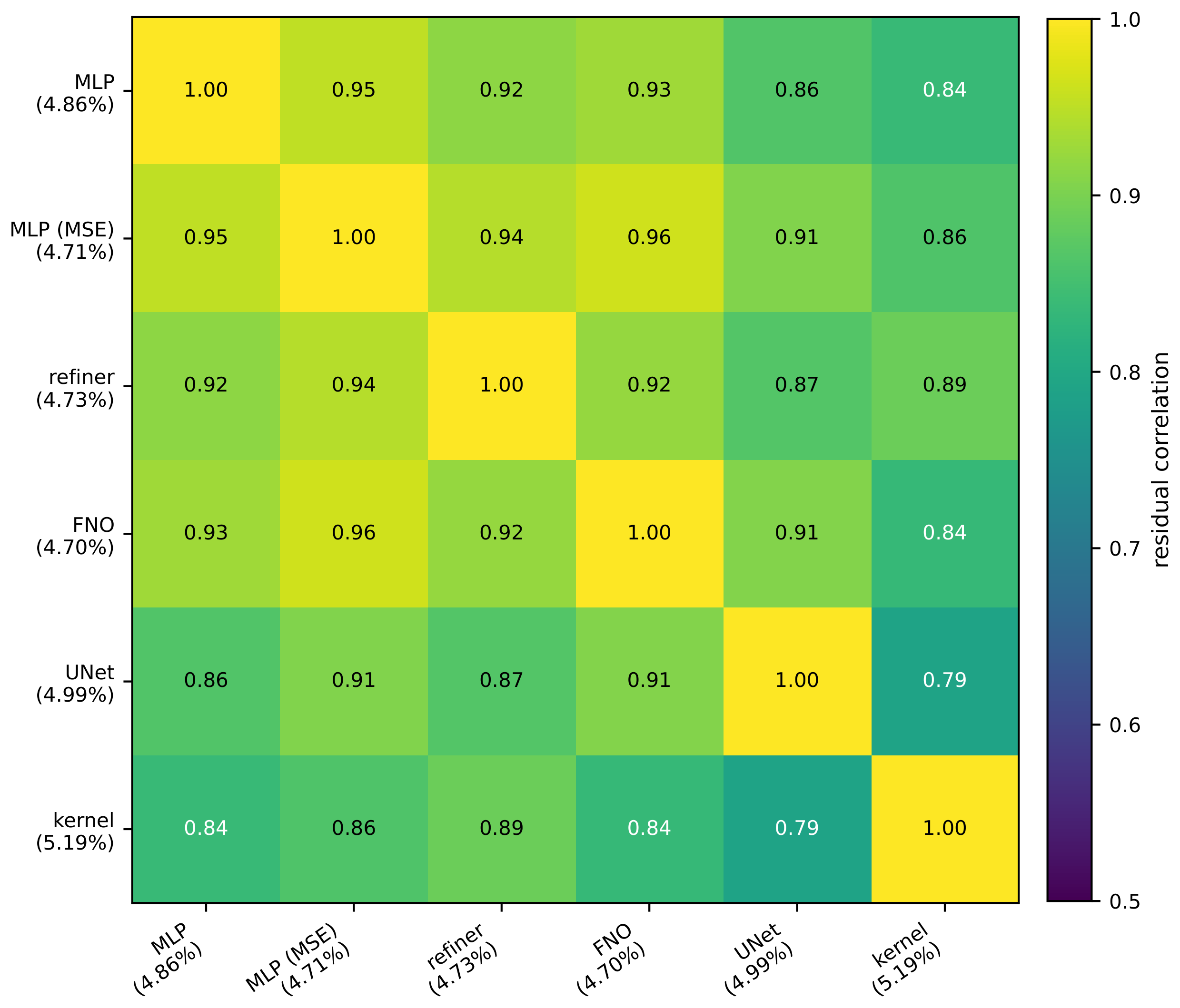
Table 2 reports the high-data protocol. The published numbers are quoted from [7] (as tabulated by [4]) and from [4]; our rows are computed under the split of Section 2, which gives our methods strictly no more training information than the baselines had. The kernel ridge row reproduces the published kernel result almost exactly (5.19% against 5.18%), which we take as evidence that the protocols are aligned; the gap opened by the rest of the pipeline is therefore not an artifact of evaluation choices. The full pipeline reaches 4.55%. This is below every published method other than PARA-Net (4.55%), which it matches at the reported two-decimal precision; since our own stacking configurations vary by a hundredth or two among themselves (the ablation below moves between 4.65% and 4.67% under changes that should not matter), we read the two as tied and do not claim to separate them. The margin over the FNO (4.76%), PCA-Net (4.67%), DeepONet (5.20%) and the optimal-recovery kernel (5.18%) is several times that spread. Section 4.3 argues the tie is better read as a floor the data impose than as a coincidence of tuning.
\begin{tabular}{lcc}
\toprule
Method & Error (\%) & Parameters \\
\midrule
DeepONet ([7]) & 5.20 & -- \\
FNO ([7]) & 4.76 & -- \\
PCA-Net ([7]) & 4.67 & -- \\
PARA-Net ([7]) & 4.55 & -- \\
Optimal-recovery kernel ([4]) & 5.18 & -- \\
\midrule
Kernel ridge on loads (ours) & 5.19 & -- \\
Residual MLP + reflection TTA & 4.86 & 4.9M \\
  + residual kernel correction (full pipeline) & 4.55 & 4.9M \\
\bottomrule
\end{tabular}
\begin{tabular}{lc}
\toprule
Method & Error (\%) \\
\midrule
DeepONet & 8.70 \\
GP, optimal recovery ([4]) & 6.95 \\
Zero-mean GP ([5]) & 6.74 \\
FNO & 6.62 \\
FNO-mean GP ([5]) & 6.49 \\
\midrule
Kernel ridge on loads (ours, multiscale) & 6.66 \\
Full pipeline (ours) & 5.38 \\
\bottomrule
\end{tabular}
4.2 Ablation
Table 4 builds the pipeline up one component at a time under the high-data protocol. The kernel ridge on loads and the reflection-averaged neural mean start at 5.19% and 4.86% respectively. Stacking is trivial with a single high-data mean and leaves it unchanged; the value of the combination appears in the correction stage, where regressing the neural mean's residual with the validated Matérn kernel lowers the error to 4.55%. The feature-space and second input-space corrections did not improve validation error beyond the first correction with a single mean and so were not selected; we expect them to contribute more with a larger and more diverse ensemble, and we report the stages that the validation split actually chose. Two smaller effects are worth isolating. Reflection test-time averaging lowers the MLP test error by 0.11 points, consistent with Proposition 1, which guarantees the direction of the change. Adding the kernel-flow regularizer (Section 6.2) to the low-data MLP did not help here (it moved test error from 5.64% to 5.87%); Proposition 2 says what the term estimates, not that estimating it is useful on every problem, and on this smooth-output benchmark the plain metric loss was already a good proxy. Nor does a richer correction kernel help: replacing the single tuned Matérn with a sum of Matérn kernels at several bandwidths leaves the validation error unchanged to two decimals, which is consistent with the residual being close to kernel-irreducible in the input geometry, and is why the boosted correction stages of Section 3.3 were not selected. One positive lesson does emerge from the refiner variants. Conditioning the refiner on the kernel method's prediction (test error 4.73%) beats conditioning it on another network's prediction (4.84%), even though the two conditioning fields have almost the same accuracy; the kernel field carries information complementary to the network's inductive bias, whereas a second network's field is largely redundant. Enlarging the ensemble beyond the residual family is the subject of the next subsection, where the returns of each addition turn out to be predictable in advance from the correlation structure of the members' errors.
: Table 4: Building the high-data pipeline. Mean relative $L^2$ test error under the 20000-sample protocol; "+" rows are cumulative.
| Stage | Test error (%) |
|---|---|
| Kernel ridge on loads | 5.19 |
| Reflection-averaged neural mean | 4.86 |
| + kernel-conditioned refiner, stack | 4.67 |
| + diverse members (Section 4.3), per-pixel stack | 4.58 |
| + residual kernel correction | 4.55 |
4.3 Architectural diversity and the shared residual
The natural reading of Table 2 is that the remaining error is a modeling problem: different architectures make different mistakes, so a more diverse ensemble should stack to a lower number. We tested this directly. To the residual family of Section 3 we added a Fourier neural operator, a UNet, and a variant of the MLP trained on normalized mean squared error instead of the metric, each trained to the published single-model level or better (Table 5). The test refutes the reading. Figure 2 shows the correlation of per-sample normalized residuals between members: every pair of trained networks, across three architecture families and two losses, correlates between 0.86 and 0.96, and the kernel predictor, the most alien member by construction, still correlates 0.79–0.89 with all of them. The members are not making different mistakes. They are making the same mistake with small private variations.
The second-moment identity of Proposition 4 makes the consequence quantitative before any weights are fitted. The matrix $S$ measured on the validation split predicts both the optimal convex weights and the achievable stack risk: for the six-member ensemble the predicted root-mean-square relative error of the best mixture is $4.97%$, the fitted stack realizes a mean of $4.61%$, and their ratio is the dispersion factor $\approx0.93$ that is stable across every pipeline we ran. The weights the prediction assigns from $S$ alone, without ever evaluating the metric, concentrated on the refiner and the FNO with a few tenths each on the UNet and the MSE-trained network, a few percent on the kernel, and zero on the plain MLP whose error is already spanned by the better members of its family, match the weights the direct metric search finds, as part (i) of the proposition predicts from the measured $(e_1, e_2, \varrho)$. Stacking does exactly what the correlations permit, and members like these permit little: part (ii) puts the infinite-ensemble floor of an equicorrelated family at $e\sqrt\varrho$, which at $e\approx4.7%$ and a mean pairwise $\varrho\approx0.9$ is about $4.5%$. Allowing the weights to vary over the grid (an affine per-pixel stack, fitted by ridge regression on half the validation split and accepted only because it beat the global weights on the other half) recovers a little of what global weights cannot see, and the kernel correction adds a few hundredths on top; that is the 4.55% of Table 2, and it is consistent with the floor just computed.
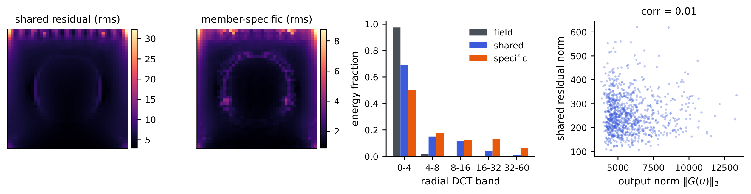
Where does the common mistake live? Write $r_m$ for member $m$ 's residual field on a validation case and $c=\frac1M\sum_m r_m$ for the across-member mean, the component that no amount of uniform averaging removes. Measured over the validation split and three families (refiner, FNO, kernel), the shared component carries $90%$ of the average residual energy (Figure 3). Three of its properties matter. Spatially, its energy concentrates at the two corners of the loaded edge, where the traction boundary condition meets the lateral supports; relative to the local field scale it is three to four times larger there than the grid average, and these are precisely the locations where the finite element solution is least accurate and where interpolation to the $41\times41$ grid is most strained. Spectrally, it is enriched in high radial frequencies relative to the stress fields themselves: the fields put $97.5%$ of their energy below radial wavenumber 4, the shared residual only $69%$. And its magnitude is statistically independent of everything we can compute from the input: the correlation of $|c|$ with the output norm is $0.01$, with the load norm $0.01$, with the load's total variation $0.01$. A component that no architecture avoids, that no input statistic predicts, that lives at the stress concentrations, and that fixed-scale additive noise would reproduce is most economically read as noise of the data-generating process itself, finite element and grid-interpolation error at the singular corners, not as approximation error of the surrogates.
Two independent measurements corroborate this reading. First, the residual kernel correction, which regresses the stack's residual on the load, improves the stack by only a few hundredths of a point at $n=19000$ whatever the kernel scale: at this sample size the shared residual is not a function of the load in any way a Matérn RKHS on $\mathbb{R}^{41}$ can see. Second, the error stops responding to data. Under identical recipes, the MLP's test error is $4.95%$ with $3500$ training samples, $4.86%$ with $8500$, and $4.86%$ with $19000$ (Figure 5); the kernel ridge curve still falls, at roughly $n^{-0.11}$, but toward the same region. A modeling limitation should yield to capacity, diversity, or data. This error yields to none of them.
We draw two conclusions. First, the published plateau of Table 2, five methods within two thirds of a point of each other after years of architectural progress, is not evidence that some sixth architecture is missing; every measurement above is what a benchmark whose achievable error is set by its data would produce. This is an inference from surrogate-side measurements — certifying it would take regenerated data, mesh-refinement checks, or repeated solver evaluations, which we did not perform — but on this reading, numbers near $4.5%$ sit within a few hundredths of the limit, which is where our pipeline lands (4.55%), and material further progress on this benchmark would come from regenerating the data (finer meshes near the corners, higher-order elements, output grids that resolve the concentrations) rather than from new surrogates. Second, the practical recipe survives the reinterpretation with its economics clarified: symmetrized accurate means capture what is learnable, stacking buys exactly the decorrelation the members possess (little, here), and the kernel correction certifies and mops up the load-visible remainder. The components are worth their cost in that order.
\begin{tabular}{llc}
\toprule
Member & Family / loss & Error (\%) \\
\midrule
Residual MLP & MLP, metric loss & 4.86 \\
Residual MLP & MLP, normalized MSE & 4.71 \\
Kernel-conditioned refiner & MLP on $(u, \mathrm{KRR}(u))$ & 4.73 \\
FNO & spectral, metric loss & 4.70 \\
UNet & convolutional, metric loss & 4.99 \\
Kernel ridge on loads & Matérn- $5/2$ & 5.19 \\
\midrule
Per-pixel stack (validation-fitted) & -- & 4.58 \\
  + residual kernel correction & -- & 4.55 \\
\bottomrule
\end{tabular}
4.4 Uncertainty quantification
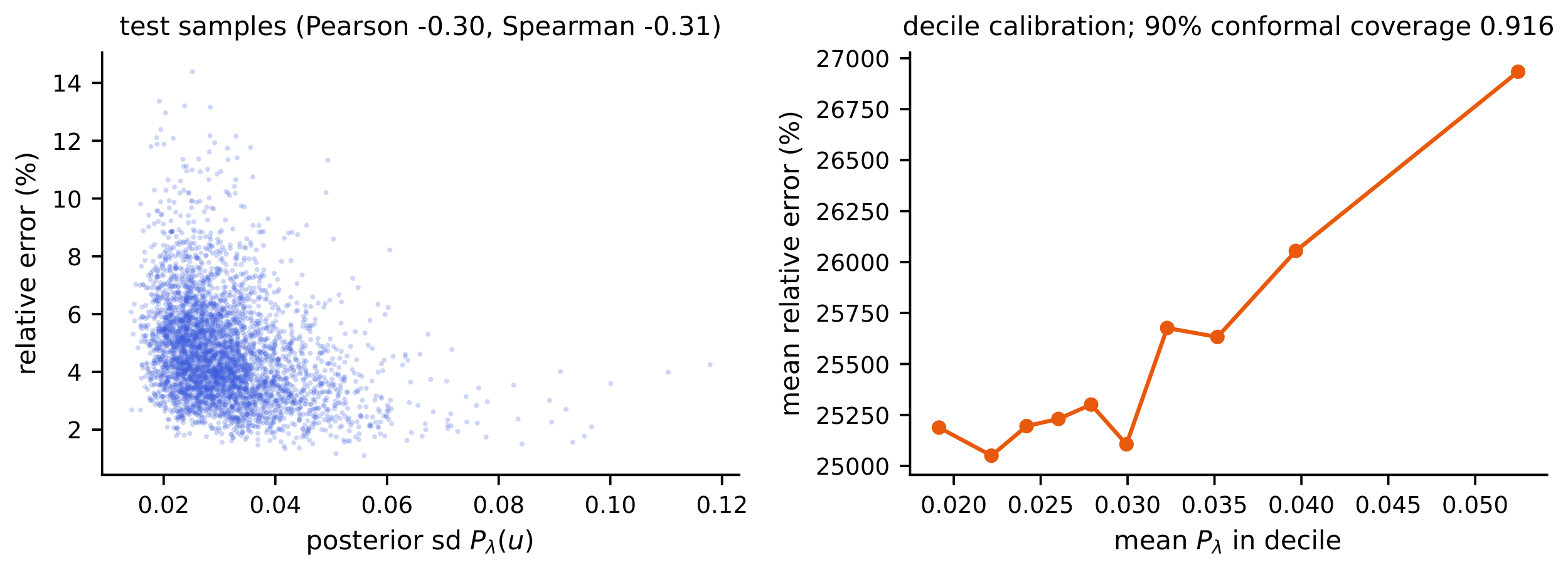
Theorem 9 certifies the corrected surrogate's error by $|G-m|K, P\lambda(u)$, and it is tempting to read the design factor $P_\lambda$ as a pointwise error bar. On this benchmark that reading fails, in an instructive way. Table 6 confirms the operator factor behaves as the theory predicts: the computable squared RKHS norm of the fitted correction is about 271 $\times$ smaller when the kernel regresses ensemble residuals than when it regresses raw stress fields, so an accurate mean genuinely leaves a smoother remainder and a tighter certificate (the bound, linear in the norm, by the square root of that). But the design factor $P_\lambda$ correlates only weakly with the corrected surrogate's absolute error (Pearson 0.08), and negatively with the benchmark's relative error. The cause is measurable: $P_\lambda$ is large for loads far from the training set, those loads tend to have large amplitude, large-amplitude loads produce large-norm stress fields, and dividing by the output norm makes their relative error small. Indeed $P_\lambda$ correlates 0.65 with the output norm (Figure 4). The error is dominated by the neural mean, whose mistakes are not a function of the input-space geometry that $P_\lambda$ sees, so a purely input-space power function cannot rank them.
The obvious alternative fares no better, and with the ensemble of Section 4.3 the question can be answered rather than left open. Ensemble disagreement, the spread of the members' predictions, is the standard deep-ensemble error signal; on the full cross-architecture ensemble its correlation with the corrected surrogate's absolute error is 0.08, no better than the 0.10 of the like-architecture ensemble. Section 4.3 says why it cannot do better here: disagreement measures the member-specific components of the error, which carry under a tenth of the residual energy, while the ranking signal for the shared component is invisible to any within-ensemble statistic, because the members agree precisely where they are jointly wrong.
What does hold is coverage, for free. A distribution-free conformal rescaling, taking the 0.9-quantile of $|e|2/P\lambda$ on the validation split and scaling $P_\lambda$ by it, yields a band with 91.6% empirical coverage on the test set at the nominal 90% level. Conformal validity needs no correlation between the score and the error, only exchangeability, so it survives the confound that defeats the ranking. One honesty note, expanded in Section 6.7: the same validation split served model selection, so the exchangeability behind the exact guarantee is approximate here, and the observed coverage should be read as empirical; a calibration split untouched by selection would make the guarantee exact. The lesson is narrow but real: a valid pointwise bound (Theorem 9) is not automatically a useful pointwise indicator, the standard uncertainty signals can both fail on the same problem, and a relative-error metric has to have its normalization accounted for before a posterior standard deviation means what it appears to.
\begin{tabular}{lc}
\toprule
Kernel regresses & $\|\widehat{r}\|_K^2$ \\
\midrule
Raw stress fields ($m=0$) & $1.39\times10^{10}$ \\
Ensemble residuals & $5.14\times10^{7}$ \\
\midrule
Ratio & 271 $\times$ \\
\bottomrule
\end{tabular}
4.5 Spectra and effective dimension
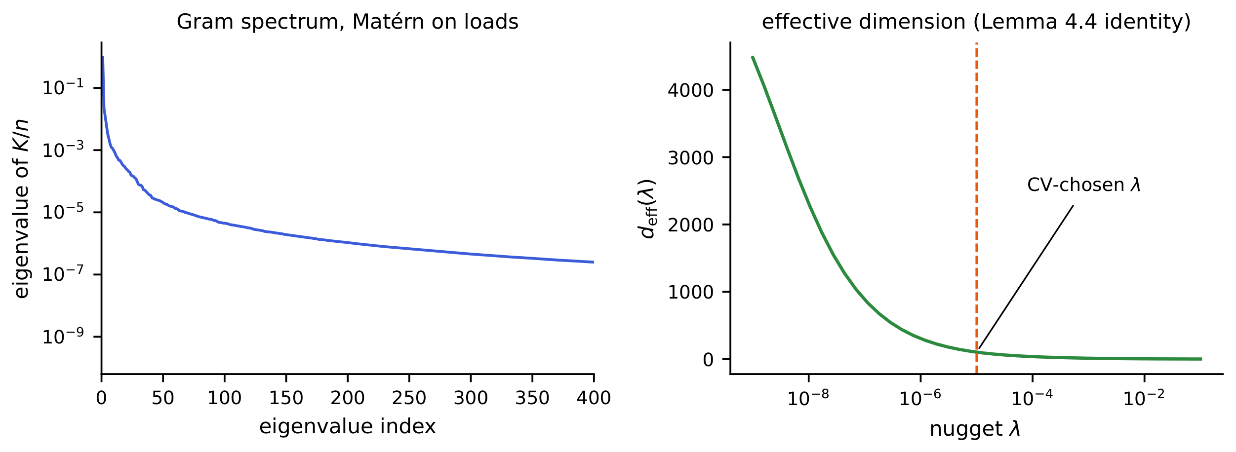
Figure 6 shows the spectrum of the Matérn Gram matrix on the loads and the effective dimension $d_{\mathrm{eff}}(\lambda)$ computed from it by the exact identity of Lemma 11. The spectrum decays quickly: a few hundred eigenvalues carry essentially all the mass, the tail falling many orders of magnitude below the leading modes. At the cross-validated nugget the effective dimension is a few hundred out of $n=19000$. This is a statistical statement, not a computational one — the dense factorization costs its full $n^3$ operations regardless — but it is why the correction generalizes despite interpolating nineteen thousand points: the problem the kernel solves has the statistical dimension of the retained spectrum, not of the sample. The cross-validated $\lambda$ sits at the shoulder of the $d_{\mathrm{eff}}$ curve, past the leading modes and into the rapidly decaying tail, matching the reading of Lemma 11.
4.6 Cost and reproducibility
The pipeline was built and run on a single laptop. The kernel stages are exact: one Cholesky factorization of the $19000\times19000$ Matérn Gram matrix in double precision takes $24$ seconds on the laptop's CPU ($16$ threads, OpenBLAS; the matrix itself is $2.9$ GB), and prediction is two matrix products; there are no inducing points, stochastic solvers, or preconditioners, and no GPU is needed for the correction. The factorization performs the full $n^3/3\approx2.3\times10^{12}$ floating-point operations — numerical low rank does not reduce the work of a dense Cholesky — and the measured rate, about $100$ gigaflops per second, is simply what a current multicore CPU delivers; exactness at this $n$ costs half a minute, not a cluster. What the low effective dimension of Section 4.5 buys is statistical rather than computational: it describes where the solve's information concentrates at the working nugget, not its flop count. The neural means are small by the standards of the literature (a few million parameters) and train in the metric itself. All splits are fixed by a published permutation seed, the input is consumed as the 41-dimensional load after the exact broadcast check of Section 2, and every model is selected on the validation split and evaluated once on the test set; we release the splits, the trained means, and the code so the table can be regenerated end to end.
5. The OCO-2 radiative-transfer emulator
Section Summary: The section applies the same neural-kernel combination to emulate radiative transfer for the OCO-2 satellite instrument, learning a map from a low-dimensional atmospheric state to 40 PCA coefficients of the radiance spectrum. It demonstrates a clear “representation ladder” in which the kernel’s error drops sharply once it operates on features from a trained residual network rather than raw inputs, and shows that a network’s training metric acts like a budget: models optimized for coefficient error or reconstructed-radiance error each excel on their own metric while losing on the other. A simple per-coordinate blend of the two networks plus their kernel heads then yields the lowest errors on both measures when scored against the previously published emulator on held-out test states.
The structural-mechanics benchmark put the neural mean and the kernel in the balanced regime. To see the other regime we apply the same components to the radiative-transfer emulation problem of [8]: per spectral band of the OCO-2 instrument, learn the map from a reduced atmospheric state ($20$ – $24$ dimensions after the dimension reduction of that paper) to the reduced radiance ($40$ PCA coefficients of the monochromatic spectrum). The OSF project (u2t8a) publishes a training pool of $20000$ pairs and, separately, $2000$ test states together with the kernel-flow emulator's own predictions on them; we verified the two sets share no point. We split the pool $18000/2000$ into training and validation, and every choice in our pipeline — the network checkpoints, the kernel head's length scale and nugget, and the per-coordinate winners of the combination below — is made on that validation split; the $2000$ public test states are used once, for the final numbers. The comparison is therefore computed on identical test points against the published emulator itself rather than against our reimplementation of it.
Two error metrics matter, and they disagree in an instructive way. The reduced metric is the relative $L^2$ error on the $40$ standardized coefficients. The radiance metric maps predictions back to the monochromatic spectrum through the stored PCA projection and norms before comparing; because the projection is orthogonal, the error numerator on the reduced side is exactly the diagonally weighted norm $|s_z\odot(\hat{z}-z)|$, whose weights concentrate almost entirely on the first few coefficients (the denominator is the full reconstructed-radiance norm, which adds the reconstruction offsets). It is this diagonal weighting of the residual that the per-coordinate combination exploits.
: Table 7: OCO-2 O2 band, scored on the $2000$ public test states, which are disjoint from the training pool; all model selection happened on a validation split of the pool. The kernel-flow row is the emulator of [8], scored from its own stored predictions. "Features" means the penultimate activations of the trained network; the kernel head is the same exact Matérn solve as everywhere else in this paper. The two raw-input rows are the diagnostic-script fit (a $6000$-point solve at a single median length scale), lighter than the feature head's full-grid fit; the anisotropy experiment of Section 6.5, which tunes the raw kernel fully, confirms it stays an order of magnitude above the feature head, so the gap is not an artifact of this.
| model | reduced | radiance |
|---|---|---|
| Matérn kernel, raw input, one length scale | 40.47% | 0.240% |
| Matérn kernel, raw input, sensitivity-scaled (ARD) | 30.01% | --- |
| kernel-flow emulator ([8]) | 16.89% | 0.0448% |
| residual MLP, flat metric | 3.99% | 0.159% |
| residual MLP, radiance metric | 46.3% | 0.0291% |
| Matérn head on the flat network's features | 3.82% | 0.0758% |
| Matérn head on the weighted network's features | 20.0% | 0.0282% |
| per-coordinate combination of the above | 3.83% | 0.0267% |
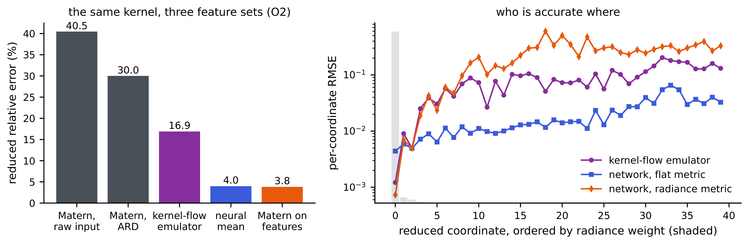
Table 7 carries four findings, and Figure 7 shows the two central ones. First, the representation ladder: the same exact kernel machinery scores $40%$ on the raw input, $30%$ after rescaling each input coordinate by its measured sensitivity (the metric term of Proposition 7: the effective rank here is $17$ of $20$, so the proposition predicts a constant-factor gain and no change of rate, the $40%!\to!30%$ the ARD row records), and $3.82%$ on the trained network's features, past the network's own head. The raw-input kernel was limited by its features, not by anything kernel-shaped, and the deep kernel head, an exact solve on learned features, is the strongest single model on the reduced metric — though its margin over the network it feeds on ($3.82%$ against $3.99%$, one seed each) is small, and we lean on the ladder's order of magnitude, not on that gap. Learning the metric rather than setting it by hand does not change this reading. A per-dimension metric fit by the kernel-flows cross-validation loss of [11] reaches the same $30%$ on the raw state, and a low-rank Mahalanobis metric with a thousand more parameters does not improve on it; on the features, where the network has already conditioned the representation, a learned metric gives no gain over the isotropic kernel. This is what Proposition 7 anticipates: the metric is a constant-factor lever, and the representation is the order-of-magnitude one.
Second, the training metric behaves as a budget. The flat-trained and radiance-trained rows are one architecture and two losses, and each wins the metric it was trained in by a factor of five or more while losing the other. The mechanism is visible per coordinate: the radiance metric concentrates on the leading coefficient, the kernel-flow emulator (whose lengthscales are tuned per output) predicts that coefficient to $0.0012$ root mean square against the flat network's $0.0054$, while the flat network is three to four times more accurate on the trailing thirty coordinates that the radiance barely sees. Training the network in the radiance metric closes exactly that gap. A constant-elasticity model of this reallocation is too crude — the per-coordinate exponents scatter widely, and coordinate errors do not decouple because the network shares capacity — but the direction is robust, and the practical rule is plain: train in the metric you report.
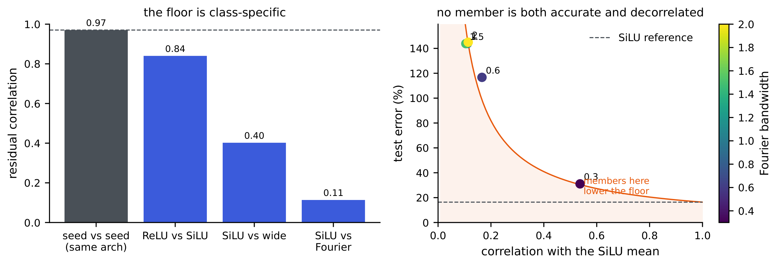
Third, the same-class floor of the structural-mechanics study reappears here, one level down. The residuals of independently seeded copies of the flat network correlate at $0.78$ on the O2 band and at $0.97$ and $0.96$ on WCO2 and SCO2, so part (ii) of Proposition 4 puts the infinite-seed floors of the flat network at $3.9%$, $16.2%$ and $8.0%$, and its seed ensemble sits there. Passing below the floor took a different kind of member: the Matérn head on learned features reaches $3.82%$, $16.1%$ and $7.96%$, and the final combination $3.83%$, $16.1%$ and $7.96%$. Ensembling within an architecture class saturates by the same second-moment law on both problems; what moved the OCO-2 numbers an order of magnitude was changing what the members are (learned features under the kernel), not how many there are.
The floor is a property of the architecture class, not of the problem, and it can be probed directly. Different architectures decorrelate: on WCO2 two residual MLPs of different activation correlate at $0.84$, a wide shallow network against the residual MLP at $0.40$, and a random-Fourier-feature network against it at $0.08$ to $0.17$, all far below the $0.96$ of two seeds. Yet the floor did not move, because its other input is accuracy: by part (i) of Proposition 4 a member of error $e_2$ helps a reference of error $e_1$ only when their correlation falls below $e_1/e_2$, and across a bandwidth sweep the Fourier network was either accurate and correlated (error $31%$, correlation $0.54$, just above the $0.53$ threshold) or decorrelated and inaccurate (error above $140%$). No architecture we tried was both accurate and decorrelated enough to lower the floor, which is the honest statement of why the residual MLP is the member of record: not that diversity is impossible, but that on this map no more accurate diverse member was found. Figure 8 shows both halves of this: the correlations that make the floor class-specific, and the accuracy-decorrelation trade-off that keeps it in place. Adding the Fourier members to the per-coordinate combination changes the reported error by less than a hundredth of a point, in either direction, on all three bands: the honesty-split blend gives them no weight.
Fourth, the regimes of Section 6.4 are decided by these numbers before any stack is fit. Against the flat network the raw-input kernel has $\varrho=0.14$ and $e_n/e_k=0.10$ (the network's $3.99%$ over the kernel's $40.47%$): the condition of Proposition 4 fails and the kernel is dropped, in contrast to structural mechanics where the same test keeps it. Because the radiance metric is diagonal in the reduced coordinates, the per-coordinate combination of Proposition 6 is optimal for both metrics simultaneously. On O2 and SCO2 this yields a single surrogate that beats the kernel-flow emulator on both metrics at once: O2 reaches $3.83%$ against $16.89%$ reduced and $0.0267%$ against $0.0448%$ radiance, and SCO2 reaches $7.96%$ against $16.14%$ reduced and $0.043%$ against $0.115%$ radiance. WCO2 is a partial exception, stated plainly. We did not produce a single combined WCO2 surrogate, and its two best heads split the metrics: the flat-feature head reaches $16.1%$ reduced, below the emulator's $24.1%$, but $0.101%$ radiance, above the emulator's $0.060%$; the radiance-trained head reaches $0.035%$ radiance but at $48%$ reduced. On WCO2, then, each metric is won by a different head, and unlike the other two bands no single model beats the emulator on both. The code releases the per-band numbers alongside this paper.
5.1 The error is limited by data, and yields to more of it
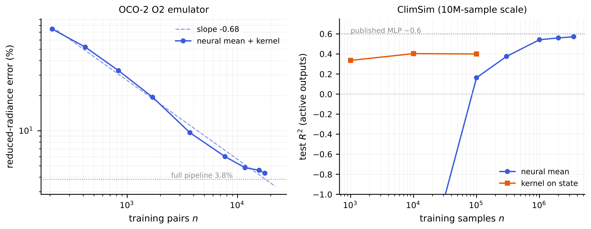
The structural-mechanics error was flat in the sample size because it is set by the noise of the finite element data; the emulator error is not, and the contrast is the sharpest practical difference between the two problems. The left panel of Figure 9 fixes the O2 task and varies only the number of training pairs, scoring each on a disjoint held-out set. The corrected surrogate's reduced-radiance error falls as a clean power law in $n$, fitted slope $-0.68$, from $74%$ at a few hundred pairs to $4.3%$ at $n=17700$, still descending at the largest sample size we can afford and approaching the $3.8%$ our full pipeline reaches on all $18000$ pairs (Table 7). The exact kernel on the raw state improves far more slowly, so at these sizes the network is the component that turns data into accuracy. The residual on this task is sample-limited rather than noise-limited: unlike the structural-mechanics floor it recedes as pairs are added, so the largest lever on this problem is simply more of them, and pairs are cheap because the forward model is a program. The complementary case is the full-resolution $58\to3048$ map, where the error is instead flat in $n$ across the few hundred retrievals we hold: that task is limited by its representation, not its sample count, and the reduction the emulator applies is what moves it.
The same reading holds well beyond OCO-2, on a benchmark large enough to watch the two regimes trade places. ClimSim ([21]) is a climate emulation dataset of about ten million samples that maps a $124$-dimensional atmospheric state to $128$ physics tendencies, with published neural baselines. The right panel of Figure 9 sweeps the training size across more than three orders of magnitude at a fixed test set, in the coefficient of determination the benchmark reports (over the outputs with non-negligible variance). The exact kernel on the state is data-efficient: its $R^2$ is already about $0.4$ at ten thousand samples and holds there. The neural mean is data-hungry: badly underfit at a thousand samples, with $R^2$ well below zero, it crosses the kernel near a few hundred thousand samples and keeps rising, reaching $R^2=0.56$ at two million and $0.57$ at three and a half million, closing on the published multilayer-perceptron baseline near $0.6$. Which member is the stronger one is therefore a matter of the sample size alone—the kernel below the crossover, the network above it—and the two regimes of Section 6.4 gain a data axis: the accurate mean is worth building precisely once there is enough data to train it past the kernel it would otherwise defer to.
6. Theory
Section Summary: The theory section supplies elementary but targeted guarantees that justify each major design choice in the operator-learning pipeline. It shows that reflection symmetrization of any predictor cannot increase the expected relative error when the underlying problem and data distribution are symmetric; that the kernel-flow regularizer is precisely an unbiased estimate, over random splits, of how well a kernel predictor built on the learned features would generalize to held-out points; and that fitting convex stacking weights or residual corrections on a modest validation split incurs negligible overfitting risk while preserving the coverage properties of the final ensemble. These statements directly underwrite the observed performance gains in the experiments.
Throughout this section $\mathcal U=\mathbb{R}^p$ denotes the (discretized) input space and $\mathcal V=\mathbb{R}^q$ the output space, $G:\mathcal U\to\mathcal V$ the target operator, $\mu$ the input distribution, and $(u_1, v_1), \dots, (u_N, v_N)$ i.i.d. draws with $v_n=G(u_n)$; the data carry no sampling noise in the usual sense, coming from a deterministic solver, though Section 4.3 has something to say about solver error. We write $\ell(w, v)=|w-v|_2/|v|2$ for the relative error and $R(\widehat{G})=\mathbb{E}{u\sim\mu}, \ell(\widehat{G}(u), G(u))$ for the risk, which is the quantity reported in Section 4. The results below are largely elementary, but each one licenses a specific design decision in the pipeline of Section 3, and each has a measurable footprint in the experiments: one statement per stage, from the symmetry handling and the kernel-flow term through stacking, the residual correction, its coverage guarantee, and the choice of nugget. Proofs are collected in Appendix A.
6.1 Symmetry averaging does not increase the risk
The elasticity problem behind the benchmark is invariant under the reflection $x_1\mapsto 1-x_1$: the domain, the boundary partition, and the constitutive model are all symmetric, the input distribution has a reflection-invariant covariance, and reflecting the load reflects the stress field. On the discrete grid this is expressed by two permutation matrices: $S\in\mathbb{R}^{p\times p}$ reverses the load samples and $T\in\mathbb{R}^{q\times q}$ reverses the rows of the stress field. Both are orthogonal involutions. Section 2 describes a direct data-driven check of the equivariance $G(Su)=T, G(u)$; we treat it as an assumption here.
########## {caption="Proposition 1: symmetrization"}
Assume $G(Su)=TG(u)$ for $\mu$-a.e. $u$, that $\mu$ is invariant under $S$, and that $T$ is an orthogonal involution ($T^2=I$). For a measurable $\widehat{G}:\mathcal U\to\mathcal V$ define its symmetrization
$ \widehat{G}_S(u);=;\tfrac12\left(\widehat{G}(u)+T, \widehat{G}(Su)\right). $
Then, for every loss $\ell(\cdot, v)$ that is convex in its first argument and satisfies $\ell(Tw, Tv)=\ell(w, v)$,
$ \mathbb{E}_{u\sim\mu}, \ell\big(\widehat{G}S(u), G(u)\big);\le; \mathbb{E}{u\sim\mu}, \ell\big(\widehat{G}(u), G(u)\big). $
The relative error satisfies both hypotheses ($T$ orthogonal gives $\ell(Tw, Tv)=\ell(w, v)$). Proposition 1 justifies the two uses of the symmetry in the pipeline: averaging each trained model with its reflected evaluation at test time can only help on average, and training on reflection-augmented data is ordinary empirical risk minimization for the symmetrized class. The measured effect is small but strictly positive for every model we trained (Table 4).
6.2 What the kernel-flow regularizer estimates
The kernel-flow (KF) loss of Owhadi and Yoo ([11]), in the $\ell^2$ variant used by [12] to regularize deep networks, enters our ablation study as an optional term in the training of the neural means. Its motivation is often stated informally ("a kernel is good if half the data predicts the rest"). The following observation makes the statement exact. Let $z_i=\phi_\theta(u_i)$ be the features of a batch $B={1, \dots, b}$ ($b$ even), let $k$ be a positive definite kernel on feature space, and for $C\subset B$, $|C|=b/2$, let $I_C$ denote the $k$-interpolant of ${(z_j, v_j):j\in C}$. The batch KF loss is
$ e_2(\theta;C);=;\sum_{i\in B}\big|v_i-I_C(z_i)\big|_2^2 .\tag{1} $
########## {caption="Proposition 2: KF loss is a leave-half-out estimate"}
Let $C$ be drawn uniformly among the subsets of $B$ of size $b/2$ and assume $k$ restricted to ${z_i}{i\in B}$ is strictly positive definite. Then $e_2(\theta;C)=\sum{i\in B\setminus C}|v_i-I_C(z_i)|_2^2$, and
$ \mathbb{E}C\big[e_2(\theta;C)\big];=;\frac b2; \mathbb{E}{C, , i, \sim, \mathrm{Unif}(B\setminus C)} \big[\big|v_i-I_C(z_i)\big|_2^2\big], $
i.e. $\tfrac2b, e_2$ is an unbiased estimator, over the split randomness, of the expected squared error committed on a held-out point by the kernel predictor trained on a random half of the batch. When $(B, C)$ are resampled at every step, the stochastic gradient $\nabla_\theta e_2(\theta;C)$ is unbiased for $\nabla_\theta, \mathbb{E}_{B, C}[e_2(\theta;C)]$ whenever the expectation and derivative commute (e.g. under local Lipschitz domination).
The training loss we minimize for a neural mean is a sum of an empirical risk term and, optionally, $\beta, e_2$: the first term is a linear functional of the empirical measure of the batch and measures fit, while Proposition 2 shows the second measures the generalization of a kernel method built on the learned features. This is the sense in which a KF-regularized network is trained to be a good feature map for the kernel correction that follows.
6.3 Stacking on a held-out split is safe
Between the means and the correction sits one more fitted object: the convex weights of the stacked ensemble, chosen to minimize the empirical risk on the validation split. Two elementary facts justify this step. First, by convexity, a convex combination of predictors is never worse than the corresponding weighted average of their risks, so stacking cannot be hurt by a weak member beyond its weight. Second, the weights live on a low-dimensional simplex and are fitted on hundreds of samples, so the selection cannot meaningfully overfit; the following proposition quantifies this with explicit constants.
########## {caption="Proposition 3: validation stacking"}
Let $f_1, \dots, f_M:\mathcal U\to\mathcal V$ be fixed maps, let $\Delta={w\in\mathbb{R}^M:w_m\ge0, \sum_m w_m=1}$, and for $w\in\Delta$ write $F_w=\sum_m w_m f_m$. Assume the members' per-sample relative errors are bounded: $\ell(f_m(u), G(u))\le B$ for $\mu$-a.e. $u$ and every $m$.
- (i) For every $w\in\Delta$, $\ell(F_w(u), G(u))\le\sum_m w_m, \ell(f_m(u), G(u))$ pointwise; in particular $R(F_w)\le\sum_m w_m R(f_m)\le\max_m R(f_m)$, and $\ell(F_w(u), G(u))\le B$.
- (ii) Let $\widehat{w}$ minimize the empirical risk $\widehat{R}(w)=\tfrac1m\sum_{i=1}^m\ell(F_w(\tilde{u}_i), G(\tilde{u}_i))$ over $\Delta$, computed on a validation sample $\tilde{u}_1, \dots, \tilde{u}_m\sim\mu$ independent of $f_1, \dots, f_M$. Then for every $\delta\in(0, 1)$, with probability at least $1-\delta$,
$ R(F_{\widehat{w}});\le;\min_{w\in\Delta}R(F_w);+;\frac{8B}{m};+; B\sqrt{\frac{2\big((M-1)\log!\big(m(M-1)+1\big)+\log(2/\delta)\big)}{m}} . $
With $M=4$ members, $m=1000$ validation samples and $\delta=0.05$ the right-hand excess evaluates to about $0.24, B$; at $B=0.25$, the largest per-sample member error we observe, this caps the selection cost at roughly six percentage points. The bound is conservative, as such bounds are: the realized validation-to-test gap of the stack in Section 4 is two orders of magnitude smaller. Its role is the scaling $\sqrt{M\log m/m}$, which says that fitting a handful of convex weights on a thousand held-out samples is statistically almost free; this is why the pipeline spends its validation data there and on the kernel hyperparameters and nowhere else.
6.4 What the stack can achieve
Proposition 3 says fitting the weights is safe; it does not say mixing is worth anything. That is decided by a single measurable matrix. For a map $f$ write the normalized residual at $u$ as $\rho_f(u)=\big(f(u)-G(u)\big)/|G(u)|_2$, so that $\ell(f(u), G(u))=|\rho_f(u)|_2$.
########## {caption="Proposition 4: second-moment identity for convex stacks"}
Let $f_1, \dots, f_M$ be fixed maps and define $S\in\mathbb{R}^{M\times M}$ by $S_{mk}=\mathbb{E}{u\sim\mu}, \langle\rho{f_m}(u), \rho_{f_k}(u)\rangle$. For $w$ in the simplex $\Delta^{M-1}$ let $f_w=\sum_m w_mf_m$. Then
$ \mathbb{E}_{u\sim\mu}, \ell\big(f_w(u), G(u)\big)^2;=;w^\top S, w, $
so the squared-metric risk of every convex stack is determined by $S$, and the best achievable is $\min_{w\in\Delta^{M-1}}w^\top Sw$. In particular:
- (i) (two members) if $S$ has diagonal $(e_1^2, e_2^2)$ with $e_1\le e_2$ and correlation $\varrho=S_{12}/(e_1e_2)$, mixing in the weaker member strictly helps if and only if $\varrho<e_1/e_2$, in which case the optimum is interior with value $e_1^2e_2^2(1-\varrho^2)/(e_1^2+e_2^2-2\varrho e_1e_2)$;
- (ii) (equicorrelated family) if $S_{mm}=e^2$ and $S_{mk}=\varrho, e^2$ for all $m\neq k$ with $\varrho\ge0$, then $\min_{w}w^\top Sw=e^2\big(\varrho+(1-\varrho)/M\big)$, attained at uniform weights and decreasing to $e^2\varrho$ as $M\to\infty$.
Exact equicorrelation never holds in practice, but for convex weights the floor survives one-sided bounds on the entries of $S$, which are what one actually measures.
########## {caption="Corollary 5: ensembling floor"}
If every member satisfies $S_{mm}\ge\bar{e}^{, 2}$ and every pair satisfies $S_{mk}\ge\bar\varrho, \bar{e}^{, 2}$ with $\bar\varrho\in[0, 1]$, then every convex combination $f_w$ obeys
$ \mathbb{E}, \ell\big(f_w(u), G(u)\big)^2;=;w^\top Sw;\ge; \bar{e}^{, 2}\big(\bar\varrho+(1-\bar\varrho), |w|_2^2\big);\ge; \bar{e}^{, 2}, \bar\varrho . $
No number of additional members with the same error level and mutual correlations moves the ensemble's root-mean-square relative error below $\bar{e}\sqrt{\bar\varrho}$.
A second consequence of the same decomposition explains the final OCO-2 surrogate. Evaluation metrics there are diagonal in the output coordinates (the radiance metric is the weighting $s_z$), and diagonal metrics decouple.
########## {caption="Proposition 6: per-coordinate combination under diagonal metrics"}
For weights $v=(v_{mj})$ that may depend on the output coordinate, let $f_v(u)j=\sum_m v{mj}f_m(u)_j$. For any diagonal metric with positive weights $w$,
$ \mathbb{E}\big|\mathrm{diag}(w)\big(f_v(u)-G(u)\big)\big|_2^2 =\sum_j w_j^2;\mathbb{E}\big(f_v(u)_j-G(u)_j\big)^2, $
so the minimizing weights solve $q$ separate problems, one per output coordinate, none of which involves $w$. The per-coordinate optimum is the same for every diagonal metric, and it weakly dominates every combination whose weights are shared across coordinates, for all such metrics simultaneously.
The practical content: when a problem is scored in several diagonal metrics at once, the combination stage does not need to know which one matters. Fit the best combination coordinate by coordinate on validation and the result serves all of them; only the members need metric-aware training, which is where the weighted mean of Section 5 enters.
The corollary is the quantity this paper keeps measuring, at two different levels. Across architecture families on the structural-mechanics benchmark the pairwise correlations exceed $0.86$ at member errors near $4.7%$, a floor of about $4.4%$, and the corrected stack lands within a tenth of it. Across random seeds of one architecture on the OCO-2 bands the correlations are $0.78$, $0.97$ and $0.96$ at member errors of $4.4%$, $16.4%$ and $8.2%$, floors of $3.9%$, $16.2%$ and $8.0%$, and the measured combinations sit on all three. When an ensemble is at its floor the corollary says where improvement cannot come from; on OCO-2 it came from changing the members (the kernel head on learned features) rather than adding more of them. The reported metric is the mean rather than the root mean square of $|\rho_f|_2$, and the two differ by the dispersion of the per-sample error; across every pipeline in this paper their ratio stays within a few percent of $0.93$, so predictions made through $S$ transfer to the reported metric essentially unchanged. The proposition frames the diversity experiment of Section 4.3: what a new member is worth is legible in the row it adds to $S$, before any weights are fitted. On this benchmark the rows all look alike, pairwise correlations of 0.86–0.96 among trained networks of three architecture families and two losses, 0.79–0.89 against the kernel predictor, so the floor sits just below the best single member, and the measured stack lands on it. Part (i) is the same computation specialized to two members; it correctly predicts, from measured $(e_1, e_2, \varrho)$ alone, which members receive weight in the fitted stack and which are dropped. Section 5 applies the same test on a problem where the answer comes out the other way: there the kernel's error is inflated by a factor the next subsection quantifies, the threshold $e_1/e_2$ collapses, and the kernel is dropped even at a residual correlation of $0.14$.
6.5 Metric and representation: when a fixed kernel loses to a network
The structural-mechanics benchmark has the neural mean and the isotropic kernel within half a point of each other. On the OCO-2 emulation problem of Section 5 the same fixed kernel is an order of magnitude behind the same network. Two mechanisms can produce such a gap, and they separate cleanly.
Suppose the operator factors as $G(u)=g(Au)$ with $A\in\mathbb{R}^{d\times d}$ nonsingular and $g$ of unit $H^{s}$ norm, and that $\mu$ has a density bounded above and below on a compact domain. Order the singular values $\sigma_1\ge\dots\ge\sigma_d$ of $A$; they are the rates at which $G$ varies along the input directions. Suppose $A$ has approximate rank $r$ at the sample size, meaning the trailing singular values fall below the achievable resolution, $\sigma_{r+1}\lesssim n^{-1/r}$, so the image $A, \mathcal U$ is effectively $r$-dimensional at scale $n^{-1/r}$.
########## {caption="Proposition 7: isotropic and adapted kernel rates"}
Let $\widehat{G}^{\mathrm{iso}}_n$ be kernel ridge regression with a Matérn kernel of smoothness $s$ and a validation-optimal single length scale, and $\widehat{G}^{\mathrm{ard}}_n$ the same construction in the metric $u\mapsto Au$. Up to constants depending on $(\sigma_i)$, $g$, $s$ and the density bounds, and up to logarithmic factors in $n$, with high probability over $n$ i.i.d. samples,
$ \mathbb{E}\big|G-\widehat{G}^{\mathrm{iso}}_n\big|;\lesssim;\sigma_1^{, s}, n^{-s/d}, \qquad \mathbb{E}\big|G-\widehat{G}^{\mathrm{ard}}_n\big|;\lesssim;n^{-s/r}, $
so the ratio of the two bounds is of order $\sigma_1^{, s}, n^{, s(1/r-1/d)}$. When $A$ is close to full rank ($r\approx d$) the two rates coincide and only the constant $\sigma_1^{, s}$ separates them.
The proof (Appendix A) is the scattered-data estimate $|G-\widehat{G}n|\lesssim h_X^{, s}|G|{H^s}$ applied to the two designs: one length scale must fill all $d$ directions, so $h_X\asymp n^{-1/d}$ and the norm carries $\sigma_1^{, s}$; the adapted metric, when $A$ has a spectral gap, confines the design to $r$ resolved directions and improves the fill distance. Both displays are upper bounds under the stated idealization — the exact metric $A$, a fixed $g$, and the length-scale selection folded into the logarithmic factors — and we claim no matching lower bound; the proposition is used here to calibrate what a metric can and cannot buy, not as a sharp rate theorem. The proposition bounds the metric part of a network's advantage, the part an anisotropic kernel would recover, and it says this part is a rate gain only under an approximate-rank gap; without one it is the constant $\sigma_1^{, s}$ alone. The rest is representational: a stationary kernel of fixed smoothness reaches only its native space, at any metric, while the network adapts its features to the map. The two parts are separated experimentally by handing the kernel the anisotropic metric and seeing how much of the gap closes. On the OCO-2 band of Section 5 the input has effective rank $17$ of $20$, close to full: the proposition predicts the metric can supply only a constant, not a rate, and the measurement agrees, $1.4$ of a tenfold gap. The remaining factor is representational, and its direct evidence is that the same kernel machinery applied to the network's learned features recovers the network's accuracy and slightly exceeds it.
The representational term has a precise reading through the same optimal-recovery bound that Section 6.6 makes exact. That bound factors the error as $|G-m|{\mathcal H}\cdot P\lambda$, a product of the target's norm in the kernel's native space and a design factor set by the Gram spectrum. Changing the features changes both in principle, but on the O2 band only one moves. The effective dimension of the Matérn Gram, the quantity Lemma 11 controls, is nearly identical on the raw input and on the learned features (at $n=4000$ and a matched median length scale, $3995$ against $3994$ at a $10^{-8}$ nugget, with equal leading eigenvalue mass), so the design factor is essentially fixed. The native-space norm of the target is not: interpolating the same outputs through the two kernels, the raw-input kernel carries the target at squared norm 1.64 x 10^6 and the feature kernel at 3.87 x 10^4, a factor of $42$. The network does not condition the kernel better; it moves the target to a low-norm corner of a native space of the same size, where the exact solve reaches it.
This is not an accident of the O2 band; it is what a pulled-back kernel does. Writing $\varphi$ for the feature map and $k$ for the base kernel, the deep kernel head uses $k_\varphi(x, x')=k(\varphi(x), \varphi(x'))$.
########## {caption="Proposition 8: feature pullback"}
The native space of $k_\varphi$ is $\mathcal H_{k_\varphi}={f\circ\varphi: f\in\mathcal H_k}$ with $|g|{\mathcal H{k_\varphi}}=\min{|f|{\mathcal H_k}: f\circ\varphi=g on \mathcal X}$. In particular, if the target factors through the features as $G=h\circ\varphi$ with $h\in\mathcal H_k$, then $|G|{\mathcal H_{k_\varphi}}\le|h|{\mathcal H_k}$, and the optimal-recovery bound of Theorem 9 for the feature-kernel regression is governed by $|h|{\mathcal H_k}$ rather than by the norm of $G$ in the raw-input space.
The proof (Appendix A) is the standard pullback identity for reproducing kernels. Its content here is the reading: a fixed kernel on the raw input must carry the whole warped map $G$, whose native-space norm is large when $G$ has fine structure; the same kernel on the features carries only the unwarped $h$, and training drives $\varphi$ toward exactly the factorization that makes $h$ simple. The measured factor of $42$ is that norm gap, and it is the representational advantage that an anisotropic metric, which rescales the input but cannot re-express the map, leaves untouched (recovering only the factor $1.4$).
6.6 An error bound for the residual kernel correction
The final stage of the pipeline is kernel ridge regression of the ensemble residual. The bound below is a vector-valued, residual form of the classical power-function estimate for kernel interpolation ([22]) and of the optimal-recovery viewpoint of [6]; we include the short argument in Appendix A to keep the two factors explicit. Fix the mean $m:\mathcal U\to\mathcal V$ (in the pipeline, the stacked ensemble; in the statement below $m$ is any fixed map independent of the correction sample) and write $r=G-m$ for the residual operator with components $r_j$, $j=1, \dots, q$. Let $k$ be a positive definite kernel on $\mathcal U$ with RKHS $\mathcal H_k$, and assume $r_j\in\mathcal H_k$ for all $j$ with
$ |r|K^2:=\sum{j=1}^q|r_j|_{\mathcal H_k}^2<\infty . $
Given inputs $X=(u_1, \dots, u_n)$, Gram matrix $K=k(X, X)$ and nugget $\lambda\ge 0$, the correction is $\widehat{r}\lambda(u)=k(u, X), (K+n\lambda I)^{-1}R$, $R{nj}=r_j(u_n)$, and the corrected predictor is $m+\widehat{r}_\lambda$. Let
$ P_\lambda(u)^2;=;k(u, u)-k(u, X), (K+n\lambda I)^{-1}k(X, u)\tag{2} $
denote the Gaussian process posterior variance with the same nugget (for $\lambda=0$ this is the classical power function of the point set $X$).
########## {caption="Theorem 9: certified pointwise bound"}
For every $u\in\mathcal U$ and every $\lambda\ge0$,
$ \big|G(u)-m(u)-\widehat{r}_\lambda(u)\big|_2;\le;|G-m|K; \widetilde{P}\lambda(u);\le;|G-m|K;P\lambda(u), $
where $\widetilde{P}\lambda(u)^2=P\lambda(u)^2-n\lambda, |(K+n\lambda I)^{-1}k(X, u)|_2^2$.
Three comments. First, the inequality is algebraic: it holds pathwise for every fixed $m$, every dataset, and every $u$, with no probabilistic assumptions. In the pipeline $m$ is itself fit on the same training set; this does not affect the validity of the bound, only the reading of $|G-m|K$ as a random (realized) quantity rather than an a priori one. Second, the bound factorizes into a quantity that depends only on the residual operator ($|G-m|K$) and a quantity that depends only on the kernel and the design ($P\lambda$), and the second factor is exactly the posterior standard deviation that a Gaussian process interpretation of the correction would report. This is the sense in which the bound is certified: whatever error the corrected surrogate commits at $u$ is controlled by the reported $P\lambda(u)$ times a constant that does not depend on $u$. We stress that this is a statement about a valid upper bound, not about the usefulness of $P_\lambda$ as a pointwise error ranking. Section 4.4 finds that on this benchmark $P_\lambda$ ranks the error poorly, because the neural mean supplies most of the error and the relative metric is confounded by output amplitude; a distribution-free conformal rescaling of $P_\lambda$ nonetheless attains its nominal coverage on the test set. Third, the theorem quantifies why one should regress residuals rather than raw targets: the design factor $P_\lambda$ is the same in both cases, so the gain of the neural mean is the drop from $|G-\bar{v}|_K$ (kernel-only, mean $\bar{v}$) to $|G-m|K$. These norms are not directly observable, but the RKHS norms of the fitted interpolants, $\smash{|\widehat{r}\lambda|_K^2=\operatorname{tr}(\alpha^\top K\alpha)}$ with $\alpha=(K+n\lambda I)^{-1}R$, are computable lower-bound proxies, and they drop by a factor of about 271 when the kernel is moved from raw targets to ensemble residuals (Table 6). The neural mean does not merely reduce the size of the residual in $L^2$; it leaves behind a residual operator that is genuinely smoother as seen by the kernel.
6.7 Distribution-free coverage for the reported band
Theorem 9 controls the error by $|G-m|K, P\lambda(u)$, but the constant $|G-m|K$ is not known a priori, and Section 4.4 shows that $P\lambda$ alone ranks the error weakly. What the surrogate reports as uncertainty is therefore not $P_\lambda$ itself but a rescaling of it, $q, P_\lambda(u)$, whose multiplier $q$ is calibrated on the held-out split by the split-conformal rule
$ q=Q_{1-\alpha}\Big(\big{s_i:=|e(\tilde{u}i)|2/P\lambda(\tilde{u}i)\big}{i=1}^m\Big), \qquad e(u)=G(u)-m(u)-\widehat{r}\lambda(u),\tag{3} $
where $Q_{1-\alpha}$ is the $\lceil(1-\alpha)(m+1)\rceil$-th smallest value of the $m$ validation scores. The point of this construction is that its coverage needs neither the bound to be tight nor $P_\lambda$ to be a good error ranking; it needs only exchangeability, which the fixed splits provide.
########## {caption="Proposition 10: finite-sample coverage"}
Fix the mean $m$, the correction $\widehat{r}\lambda$ and the design $X$, and let $P\lambda(\cdot)>0$. Suppose the validation and test inputs $\tilde{u}1, \dots, \tilde{u}m, u^\star$ are exchangeable (in particular i.i.d. from $\mu$) and drawn independently of $m, \widehat{r}\lambda, X$. Let $q$ be the conformal multiplier Equation 3 and define the band $C(u)={v:|v-m(u)-\widehat{r}\lambda(u)|2\le q, P\lambda(u)}$. Then
$ 1-\alpha;\le;\mathbb{P}\big(G(u^\star)\in C(u^\star)\big);\le; 1-\alpha+\frac{1}{m+1}, $
the upper bound holding when the scores are almost surely distinct.
The two-sided statement is the standard guarantee of split conformal prediction ([23, 24]), transported to the functional-output setting by taking the nonconformity score to be the relative residual norm $s=|e(u)|2/P\lambda(u)$; the proof, a rank argument on the exchangeable scores, is in Appendix A. Three points make it the right closing statement for the uncertainty analysis. It is close to the quantity we compute: the reported coverage of 91.6% at the nominal $1-\alpha= 90%$ in Section 4.4 realizes this proposition with $m=1000$ and $\alpha=0.1$. The $1.6$-point excess over nominal is not the $1/(m+1)$ slack, which is only a tenth of a point; it is the finite-sample fluctuation of coverage on a single test set, whose standard deviation $\sqrt{\alpha(1-\alpha)/m}\approx0.95$ point places 91.6% about $1.7$ standard deviations above nominal, well inside the guarantee. One caveat on the hypotheses: our calibration scores are computed on the same held-out split used to select the neural-mean checkpoints and tune the correction, so the exchangeability the proposition assumes is only approximate here; the selection is low-complexity and the band over-covers, but a calibration split disjoint from model selection would make the guarantee exact. It is agnostic to everything the earlier results leave uncertain: the neural mean may be biased, $P_\lambda$ may correlate with the error weakly or with the wrong sign, and the bound of Theorem 9 may be loose, yet the band still covers at the stated rate. And it is where the uncertainty analysis ends: among the candidate uncertainty signals we examine, the conformally rescaled $P_\lambda$ is the only one that carries a guarantee, so it is the one the surrogate reports.
6.8 Effective dimension from the Gram spectrum
The remaining design choice is the nugget $\lambda$, selected by cross-validation in the pipeline. The following exact identity connects that choice to the spectrum of the Gram matrix and, through it, to random matrix descriptions of the design.
########## {caption="Lemma 11: effective dimension and the empirical Stieltjes transform"}
Let $K$ be a symmetric positive semidefinite $n\times n$ matrix with eigenvalues $\lambda_1, \dots, \lambda_n\ge0$, let $\widehat{m}(z)=\tfrac1n\sum_{i=1}^n(\lambda_i/n-z)^{-1}$ be the Stieltjes transform of the empirical spectral distribution of $K/n$. Then for every $\lambda>0$ the effective dimension of ridge regression with nugget $\lambda$ satisfies
$ d_{\mathrm{eff}}(\lambda);:=;\operatorname{tr}!\big(K(K+n\lambda I)^{-1}\big) ;=;n\big(1-\lambda, \widehat{m}(-\lambda)\big). $
In particular, if the empirical spectral distribution of $K/n$ converges weakly to a limit law $F$ as $n\to\infty$, then $d_{\mathrm{eff}}(\lambda)/n\to 1-\lambda, m_F(-\lambda)$ with $m_F$ the Stieltjes transform of $F$.
The identity is unconditional; the random-matrix content enters through the choice of $F$. For the benchmark's simplest reference model, isotropic linear features, the limit can be evaluated in closed form.
########## {caption="Corollary 12: effective dimension under a Marčenko–Pastur limit"}
Let $K=XX^\top$ with $X\in\mathbb{R}^{n\times p}$ having i.i.d. entries of mean zero and variance $\sigma^2$, and let $p/n\to\gamma\in(0, 1]$. Then
$ \frac{d_{\mathrm{eff}}(\lambda)}{n};\longrightarrow; \gamma\big(1-\lambda, m(-\lambda)\big), \qquad m(-\lambda)=\frac{\sqrt{\big(\lambda+\sigma^2(1-\gamma)\big)^2+4\gamma\sigma^2\lambda} -\big(\lambda+\sigma^2(1-\gamma)\big)}{2\gamma\sigma^2\lambda}, $
almost surely, where $m$ is the Stieltjes transform of the Marčenko–Pastur law with ratio $\gamma$ and scale $\sigma^2$. In a simulation with $n=6000$, $p=1800$, $\sigma^2=1.7$, the formula agrees with the empirical $d_{\mathrm{eff}}(\lambda)/n$ to four decimal places across $\lambda\in[10^{-3}, 10]$.
Two uses. Quantitatively, the formula makes the nugget–capacity trade-off explicit for the bulk of a feature Gram matrix: eigenvalue mass of Marčenko–Pastur type is absorbed or discarded by $\lambda$ according to a single closed-form curve, and outlying (spiked) eigenvalues $x_s$ simply add their terms $x_s/(x_s+n\lambda)$ on top. Qualitatively, it separates the two regimes visible in Figure 6: the Matérn Gram matrix on the loads is nothing like a Marčenko–Pastur bulk (its spectrum decays exponentially, which is why $d_{\mathrm{eff}}$ is a few hundred out of 19000), whereas the Gram matrices of learned penultimate features do show a bulk-plus-spikes shape, and for them the corollary describes how much of the bulk the cross-validated nugget retains. For the feature Gram matrices of the trained networks we observe the familiar picture of a bulk that is well fitted by a Marčenko–Pastur law ([15]) together with a small number of outlying eigenvalues carrying the regression signal, as in spiked covariance models ([16]); for the Matérn Gram matrix on the 41-dimensional loads the spectrum decays rapidly and $d_{\mathrm{eff}}$ is small ($\approx$ a few hundred at the cross-validated $\lambda$, out of $n=19000$; Figure 6). This gives a post-hoc reading of the cross-validated nugget: $\lambda$ lands where $d_{\mathrm{eff}}(\lambda)$ has absorbed the outlying eigenvalues and the leading bulk, and further decreasing $\lambda$ buys capacity precisely where the spectrum carries little signal. It also explains why the exact solve is affordable: the correction is numerically a problem of dimension $d_{\mathrm{eff}}$, not $n$.
The effective dimension is also exactly the total budget of the design factor from Theorem 9. Writing $A=K+n\lambda I$, the posterior variances at the training inputs sum to
$ \sum_{i=1}^{n}P_\lambda(u_i)^2 =\operatorname{tr}(K)-\operatorname{tr}(K A^{-1}K) =\operatorname{tr}!\big(n\lambda, KA^{-1}\big) =n\lambda, d_{\mathrm{eff}}(\lambda), $
using $KA^{-1}K=K-n\lambda, KA^{-1}$. So the same $d_{\mathrm{eff}}$ that reads the nugget off the spectrum also fixes, up to the factor $n\lambda$, the total posterior-variance mass the correction distributes over the design; the two halves of this section are one quantity seen from two sides.
7. Discussion
Section Summary: The gains over prior results come mostly from training accurate neural networks on the target metric and averaging predictions across symmetric variants, with smaller further lifts obtained by combining models from different families and applying lightweight kernel corrections afterward. Progress beyond this point is blocked by a shared source of error that appears in every architecture, concentrates in regions where the underlying data are least reliable, and cannot be removed by adding capacity, diversity, or more samples. The overall pipeline is consistent with earlier neural-Gaussian-process and large-scale kernel emulation work, though it differs in fitting order and validation choices; its practical limits are set by the one-dimensional benchmark geometry and by how closely the residual error can be bounded.
What moved the number, and what stopped it.
The improvement over the published band decomposes unevenly. Accurate neural means trained on the reported metric and averaged over the reflection symmetry do most of the work; stacking members from different architecture families adds exactly what their measured residual correlations permit, about a tenth of a point here; the kernel corrections contribute a few hundredths more and, with them, the certificate of Theorem 9 and the calibrated band of Proposition 10. We did not find evidence that any published architecture was mis-tuned by its authors; the components compose, and the composition had not been tried on this benchmark. What stops further movement is not a missing architecture. Section 4.3 locates the remaining error in a component that all families share, that concentrates where the finite element data are least reliable, that no input statistic predicts, and that neither capacity, nor diversity, nor more data reduces. The margin over the published methods other than PARA-Net is real, and the match with PARA-Net is exact to within run-to-run noise, but both should be read for what they are: the last few learnable hundredths above what the evidence of Section 4.3 reads as a data-set floor, not a step on the way to zero.
Relation to neural-mean Gaussian processes.
Our correction stage is closest in spirit to [5], who place a neural operator inside the mean of a Gaussian process and fit both jointly. The differences are operational but they matter at this scale: we fit the mean first and the kernel after (so the expensive stage is ordinary network training), we tune the kernel by validation rather than by marginal likelihood, we correct with an exact solve at $n=19000$ rather than train through the kernel, and we add the feature-space second stage. The theory in Section 6 applies verbatim to their setting as well; the measured drop in the fitted RKHS norm (Table 6) is the quantitative reason residual corrections of accurate means are the right place to spend kernel capacity.
Relation to kernel emulation practice.
The pipeline is consistent with the experience of the kernel-flow line of work in emulation at scale. The closest instance is the forward-model emulator of [8] for the OCO-2 CO$_2$ retrievals, in which a Gaussian process with a cross-validation-learned kernel replaces the full-physics radiative transfer code within measurement-error precision; kernel flows have likewise been used to infer convective-storm structure from passive microwave observations ([13]). The lesson of that work matches ours: kernels with data-adapted hyperparameters are extremely effective once the input is presented in its physical parametrization and the target has been reduced to something smooth. Here the reduction is performed by the neural ensemble rather than by physics, and the kernel-flow loss itself admits the leave-half-out reading of Proposition 2. The OCO-2 setting is also the natural next test bed for the residual coupling studied here. Its training pairs are simulator-generated state-to-radiance maps of exactly the shape this paper exploits, a low-dimensional physical state mapped to a smooth high-dimensional output, the mission's Level 1 and Level 2 products are publicly distributed through NASA's Earthdata archive, and the emulation setup of [8] specifies the state parametrization and sampling design, so a neural mean with a validated kernel correction and a conformal wrapper can be evaluated there against the pure-kernel emulator without new data collection.
Limitations.
The benchmark has a one-dimensional input function and a fixed geometry; the exact kernel solve exploits both, and problems with high-dimensional input fields would require the usual approximations (inducing points, random features) at some cost to the certificates. The certified bound of Theorem 9 controls the error relative to the RKHS norm of the residual operator, a quantity we can only lower-bound empirically; the conformal calibration we report is the honest, assumption-light complement. Training the means on the metric, the reflection steps, and the stacking are benchmark-agnostic, but the specific error levels reported here should be read as properties of this dataset and protocol. Finally, our low-data protocol reproduces that of [5] up to the unavoidable ambiguity of which 1250 samples are used; we use the first 1250 of the training block and report the same 20000-sample test set, and we release splits and code so the comparison can be audited.
What the second problem settles.
The OCO-2 study keeps every component and inverts the balance, and the pair of problems brackets the design space. When the network and the kernel tie (structural mechanics), the coupling pays: stack them, correct the residual, and the certified and conformal machinery rides along. When the kernel trails by an order of magnitude (OCO-2), the coupling is not the point; the kernel's value moves inside the network, as an exact head on its learned features, and the pipeline's job becomes metric management, training each member in the metric it will be scored in and combining per coordinate. In both regimes the same two measurements decide everything in advance: the pairwise residual correlations, which set the ensembling floor of Corollary 5 at whatever level the members share their errors, and the member error ratio, which the second-moment identity turns into a keep-or-drop verdict for each candidate. Nothing in that protocol is specific to these two datasets.
Outlook.
Three directions seem worth pursuing. First, the benchmark itself: regenerating the dataset with refined meshes at the corner singularities, higher-order elements, or output grids that resolve the concentrations would move the floor that Section 4.3 measures, and would return the problem to being a test of surrogates rather than of its own data. The diagnostic protocol used there, cross-family residual correlation, the second-moment prediction of Proposition 4, and the scaling-in- $n$ check, is cheap to run on any benchmark suspected of the same condition. Second, the same recipe on the remaining benchmarks of [7] and [4], where the input functions are genuinely high-dimensional and the interplay between neural means and kernel corrections should look different. Third, the uncertainty side: $P_\lambda$ is a design quantity, so it can be optimized, and the connection of Lemma 11 between the nugget, the spectrum, and the effective dimension suggests principled ways to spend a fixed computational budget on the correction stage.
Acknowledgments and funding
Section Summary: The research described in the paper was funded by several organizations, including the European Research Council under a European Union program and the Simons Foundation as part of a collaboration focused on deep learning. It also received support from Heights Labs along with two grants from the Israel Science Foundation. Additional backing came from the U.S. National Science Foundation.
The research presented in this paper was supported by the European Research Council (ERC) under the European Union's Horizon 2022 research and innovation programme (grant agreement No. 101041711), by the Simons Foundation as part of the Collaboration on the Mathematical and Scientific Foundations of Deep Learning, by Heights Labs, by the Israel Science Foundation (grant number 2258/19), by the Israel Science Foundation (ISF Grant 4101/25), and by the U.S. National Science Foundation (NSF Grant OISE-2401227).
Declaration of competing interest
The author declares no competing interests.
Declaration of generative AI and AI-assisted technologies in the manuscript preparation process
Section Summary: The author relied heavily on generative AI tools during the creation of this paper. Most of the software code, data preparation, and adaptation of existing emulator programs were produced with Fable 5 from Anthropic, while ChatGPT also helped with calculations, drafting sections, and verifying the mathematical proofs and numerical results. The core scientific ideas, framing, and final responsibility for the work remain with the author.
During the preparation of this work the author made substantial use of generative AI tools, and describes their role here. A large part of the software was written with Fable 5 (Anthropic): the implementation of the experiments and diagnostics, the downloading, assembly and preparation of the benchmark and OCO-2 datasets, and the adaptation of the publicly released emulator code of Lamminpää et al. — originally split between Julia and a ReFRACtor-driving Python layer — into a single Python pipeline for sampling states and reducing radiances. The main contributions are the author's: the residual coupling of neural means and exact kernel corrections, the two-regime framing that organizes the paper, and the supporting theory, all developed with AI assistance in calculation, drafting, and exposition. Each theorem and its proof was checked independently and more than once — by Fable 5, by ChatGPT Pro (OpenAI), and by the author — and the reported numbers were verified against the released per-run data. The author reviewed all of the above and takes full responsibility for the content of the manuscript.
Data and code availability
Section Summary: All the computer code, detailed experiment settings, and supporting summaries of results are freely available in a public GitHub repository. The different datasets used in the work, covering structural mechanics, fluid flow, satellite observations, and climate simulations, are shared through established online archives at Caltech, OSF, and the LEAP repository.
The code, the per-run summaries behind every reported number, and the exact configuration of each experiment are available at https://github.com/yspennstate/neural-means-kernel-corrections. The structural-mechanics, Helmholtz, Navier–Stokes and advection data are distributed through the data record accompanying [7] (data.caltech.edu, record 20091); the OCO-2 emulation data and the kernel-flow emulator's predictions through the OSF project u2t8a; and the ClimSim data through the LEAP repository subsampled_low_res.
Appendix
Section Summary: The appendix presents rigorous mathematical proofs for six propositions and one corollary that establish key theoretical properties of the paper's main results. These include showing that certain averaged predictors achieve lower or equal expected loss through convexity and symmetry arguments, deriving exact expressions for interpolation errors and their gradients under kernel methods, and proving risk bounds for convex combinations of models via Lipschitz analysis, discretization of the weight simplex, and concentration inequalities. Additional proofs characterize optimal weighting schemes that minimize quadratic residual forms and establish related lower bounds under correlation assumptions.
A. Proofs
A.1 Proof of Proposition 1
By convexity of $\ell(\cdot, v)$,
$ \ell\big(\widehat{G}_S(u), G(u)\big);\le;\tfrac12, \ell\big(\widehat{G}(u), G(u)\big)+\tfrac12, \ell\big(T\widehat{G}(Su), G(u)\big). $
Since $T$ is an involution, the equivariance $G(Su)=TG(u)$ applied at $u$ gives $TG(Su)=T^2G(u)=G(u)$, hence
$ \ell\big(T\widehat{G}(Su), G(u)\big)=\ell\big(T\widehat{G}(Su), TG(Su)\big) =\ell\big(\widehat{G}(Su), G(Su)\big), $
using the $T$-invariance of the loss. Taking expectations and using the $S$-invariance of $\mu$ (so that $Su\sim\mu$ when $u\sim\mu$),
$ \mathbb{E}, \ell\big(\widehat{G}_S(u), G(u)\big)\le\tfrac12, \mathbb{E}, \ell\big(\widehat{G}(u), G(u)\big)+\tfrac12, \mathbb{E}, \ell\big(\widehat{G}(Su), G(Su)\big)=\mathbb{E}, \ell\big(\widehat{G}(u), G(u)\big). \blacksquare $
A.2 Proof of Proposition 2
Strict positive definiteness of the restricted kernel matrix makes $I_C$ the (unique) interpolant of the pairs indexed by $C$, so $I_C(z_j)=v_j$ for $j\in C$ and the terms of Equation 1 indexed by $C$ vanish, which is the first claim. For the second, write
$ e_2(\theta;C);=;\sum_{i\in B\setminus C} g(C, i), \qquad g(C, i):=|v_i-I_C(z_i)|_2^2 . $
Conditionally on $C$, the sum has exactly $b/2$ terms, so $e_2(\theta;C)=\tfrac b2, \mathbb{E}{i\sim\mathrm{Unif}(B\setminus C)}[g(C, i)]$, and taking the expectation over $C$ proves the identity. The gradient claim is immediate: for fixed $(B, C)$ the map $\theta\mapsto e_2(\theta;C)$ is differentiable wherever the Cholesky factorization in $I_C$ is (the kernel matrix stays positive definite in a neighborhood), and under a local integrable Lipschitz bound the derivative passes under the expectation, so $\mathbb{E}{B, C}[\nabla_\theta e_2]=\nabla_\theta, \mathbb{E}_{B, C}[e_2]$. $\blacksquare$
A.3 Proof of Proposition 3
(i) Since $\sum_m w_m=1$, $F_w(u)-G(u)=\sum_m w_m, (f_m(u)-G(u))$, and the triangle inequality gives $|F_w(u)-G(u)|_2\le\sum_m w_m|f_m(u)-G(u)|_2$. Dividing by $|G(u)|_2$ yields the pointwise claim; taking expectations gives the risk inequality, and bounding each $\ell(f_m(u), G(u))$ by $B$ gives $\ell(F_w(u), G(u))\le B$.
(ii) Write $\ell_u(w)=\ell(F_w(u), G(u))$. First, $\ell_u$ is Lipschitz on $\Delta$ for the $\ell^1$ norm: for $w, w'\in\Delta$, the reverse triangle inequality and the argument of (i) give
$ |\ell_u(w)-\ell_u(w')|;\le;\frac{\big|\sum_m (w_m-w'_m)(f_m(u)-G(u))\big|_2} {|G(u)|_2};\le;B, |w-w'|_1 . $
Next, discretize the simplex. For $k\in\mathbb{N}$ let $\mathcal G_k={w\in\Delta:, kw\in\mathbb{Z}^M}$; its cardinality is the number of compositions of $k$ into $M$ nonnegative parts, $\binom{k+M-1}{M-1}\le (k+1)^{M-1}$. Given $w\in\Delta$, set $w'_i=\lfloor kw_i\rfloor/k$ for $i<M$ and $w'M=1-\sum{i<M}w'_i$; then $w'\in\mathcal G_k$ (the last coordinate is a multiple of $1/k$ and is $\ge w_M\ge0$ because the first $M-1$ coordinates only decreased), and
$ |w-w'|1=\sum{i<M}(w_i-w'_i)+\big(w'M-w_M\big) =2\sum{i<M}(w_i-w'_i);\le;\frac{2(M-1)}{k}. $
By (i) the per-sample loss lies in $[0, B]$, so for each fixed $w'$ Hoeffding's inequality gives $\mathbb{P}\big(|\widehat{R}(w')-R(w')|>t\big)\le2e^{-2mt^2/B^2}$, and a union bound over $\mathcal G_k$ shows that with probability at least $1-\delta$,
$ \sup_{w'\in\mathcal G_k}\big|\widehat{R}(w')-R(w')\big|;\le; B\sqrt{\frac{\log!\big(2|\mathcal G_k|/\delta\big)}{2m}} . $
On this event, for every $w\in\Delta$, approximating by its grid point and using the Lipschitz property for both $R$ and $\widehat{R}$,
$ \big|\widehat{R}(w)-R(w)\big|;\le; B\sqrt{\frac{\log(2|\mathcal G_k|/\delta)}{2m}}+\frac{4B(M-1)}{k}. $
If $w^\star$ minimizes $R$ over $\Delta$, the empirical minimizer satisfies $R(F_{\widehat{w}})\le\widehat{R}(\widehat{w})+\sup_\Delta|\widehat{R}-R| \le\widehat{R}(w^\star)+\sup_\Delta|\widehat{R}-R| \le R(F_{w^\star})+2\sup_\Delta|\widehat{R}-R|$. Choosing $k=m(M-1)$ and using $|\mathcal G_k|\le(m(M-1)+1)^{M-1}$ gives
$ R(F_{\widehat{w}});\le;\min_{w\in\Delta}R(F_w)+\frac{8B}{m} +B\sqrt{\frac{2\big((M-1)\log(m(M-1)+1)+\log(2/\delta)\big)}{m}}, $
which is the claim. $\blacksquare$
A.4 Proof of Proposition 4
Since $\sum_m w_m=1$, the stack's normalized residual is $\rho_{f_w}(u)=\sum_m w_m\rho_{f_m}(u)$, hence
$ \mathbb{E}, \ell\big(f_w(u), G(u)\big)^2 =\mathbb{E}\Big|\sum_m w_m\rho_{f_m}(u)\Big|2^2 =\sum{m, k}w_mw_k, \mathbb{E}, \langle\rho_{f_m}(u), \rho_{f_k}(u)\rangle =w^\top Sw . $
For (i), parameterize $w=(1-t, t)$; $q(t)=w^\top Sw$ is a convex quadratic in $t$ with $q'(0)=2(\varrho e_1e_2-e_1^2)$, negative precisely when $\varrho<e_1/e_2$. In that case the unconstrained minimizer lies in $(0, 1)$ and gives the stated interior value; otherwise $q'(0)\ge0$, the minimum over $[0, 1]$ is at $t=0$ with value $e_1^2$, and the second member is dropped. For (ii), $S=e^2\big((1-\varrho)I+\varrho, \mathbf1\mathbf1^\top\big)$, so $w^\top Sw=e^2\big((1-\varrho)|w|_2^2+\varrho\big)$ on the simplex, minimized by the uniform weights, where $|w|_2^2=1/M$. $\blacksquare$
A.5 Proof of Corollary 5
Convex weights are nonnegative, so each term of $w^\top Sw=\sum_{m}w_m^2S_{mm}+\sum_{m\neq k}w_mw_kS_{mk}$ can be bounded below entrywise:
$ w^\top Sw;\ge;\bar{e}^{, 2}\sum_m w_m^2+\bar\varrho, \bar{e}^{, 2}\sum_{m\neq k}w_mw_k =\bar{e}^{, 2}\Big(|w|_2^2+\bar\varrho, (1-|w|_2^2)\Big), $
using $\sum_{m\neq k}w_mw_k=(\sum_m w_m)^2-|w|_2^2=1-|w|_2^2$. The bracket is a convex combination of $1$ and $\bar\varrho$, hence at least $\bar\varrho$. $\blacksquare$
A.6 Proof of Proposition 6
The metric is diagonal, so the squared norm splits over coordinates and the $j$-th summand $w_j^2, \mathbb{E}\big(\sum_m v_{mj}f_m(u)j-G(u)j\big)^2$ depends on the weights only through the column $v{\cdot j}$. Minimizing the sum is therefore $q$ independent minimizations, and the positive factor $w_j^2$ does not move any of the $q$ argmins, so the optimizer is the same for every positive $w$. A combination with shared weights is the special case $v{mj}=v_m$ for all $j$, a subset of the feasible set of each coordinate problem, which gives the domination. $\blacksquare$
A.7 Proof of Proposition 8
Let $T:\mathcal H_k\to\mathbb{R}^{\mathcal X}$ be the composition map $Tf=f\circ\varphi$. For $x\in\mathcal X$ the reproducing property gives $(Tf)(x)=f(\varphi(x))=\langle f, k(\cdot, \varphi(x))\rangle_{\mathcal H_k}$, so evaluation of $Tf$ at $x$ is a bounded functional, and the image $\mathcal H_{k_\varphi}:=T(\mathcal H_k)$ carries the quotient norm $|g|{\mathcal H{k_\varphi}}=\min{|f|{\mathcal H_k}:Tf=g}$, the minimum over the affine subspace $T^{-1}(g)$ (nonempty exactly when $g$ is a pullback). This normed space is an RKHS: its reproducing kernel is $k\varphi(x, x')=\langle k(\cdot, \varphi(x)), k(\cdot, \varphi(x'))\rangle_{\mathcal H_k} =k(\varphi(x), \varphi(x'))$, since the minimum-norm representer of evaluation at $x$ is $k(\cdot, \varphi(x))$. Taking $f=h$ in the minimum gives $|h\circ\varphi|{\mathcal H{k_\varphi}}\le|h|{\mathcal H_k}$, and substituting this bound into Theorem 9 applied with the kernel $k\varphi$ replaces $|G|$ by $|h|_{\mathcal H_k}$. $\blacksquare$
A.8 Proof of Proposition 7
Both displays are the native-space estimate for kernel ridge regression: for a Matérn kernel of smoothness $s$ on a bounded domain, with the nugget chosen as in the pipeline, an estimator $\widehat{G}_n$ of a target $F$ in the native space obeys $\mathbb{E}|F-\widehat{G}n|\le C, h_X^{, s}, |F|{\mathcal N}$, with $h_X$ the fill distance of the design in the kernel's metric ([22]), and for $n$ samples from a density bounded above and below on a set of effective dimension $d'$, quasi-uniformity gives $h_X\asymp(\log n/n)^{1/d'}$ with high probability, which we write as $n^{-1/d'}$ up to the logarithmic factor absorbed into the statement.
For the isotropic kernel the metric is Euclidean on the full $d$-dimensional domain, so $h_X\asymp n^{-1/d}$; the target is $F=g(A, \cdot)$, whose Matérn native norm is equivalent to its $H^{s}$ norm. Changing variables $y=Au$ gives $|g(A\cdot)|{H^{s}}\asymp|\det A|^{-1/2}, \sigma_1^{, s}$, since each derivative of order up to $s$ brings down at most a factor $\sigma_1$ and the Jacobian contributes $|\det A|^{-1/2}$ in $L^2$; the $|\det A|^{-1/2}$ is one of the singular-value constants absorbed into the statement, leaving the displayed $\sigma_1^{, s}$. For the adapted kernel $k_A(u, u')=k(Au, Au')$ the estimator is the isotropic estimator of the unit-norm $g$ on the design ${Au_i}$. Here the approximate-rank hypothesis enters: the design $A, \mathcal U$ has extent $\sigma{r+1}\lesssim n^{-1/r}$ in each of the trailing $d-r$ directions, below the fill distance those directions would otherwise demand, so at resolution $n^{-1/r}$ the design is $r$-dimensional and its fill distance is $h_X\asymp n^{-1/r}$ (a further $(\prod_{i\le r}\sigma_i)$ constant, again absorbed). Substituting the two fill distances into the native-space estimate and dividing gives the ratio. If instead $A$ is close to full rank, $\sigma_{r+1}$ is not below $n^{-1/r}$, the trailing directions are resolved, and the adapted fill distance is $n^{-1/d}$ like the isotropic one: the rates coincide and only $\sigma_1^{, s}$ separates the bounds. $\blacksquare$
A.9 Proof of Theorem 9
Fix $u$ and write $\kappa=k(X, u)\in\mathbb{R}^n$, $A=K+n\lambda I$, $w=A^{-1}\kappa$. For each component $j$, membership $r_j\in\mathcal H_k$ and the reproducing property give
$ r_j(u)-\widehat{r}{\lambda, j}(u) = \Big\langle r_j, ; k(u, \cdot)-\sum{i=1}^n w_i, k(u_i, \cdot)\Big\rangle_{\mathcal H_k}, $
because $\widehat{r}_{\lambda, j}(u)=\kappa^\top A^{-1}r_j(X)=\sum_i w_i, r_j(u_i)$ and $r_j(u_i)=\langle r_j, k(u_i, \cdot)\rangle$. Cauchy–Schwarz yields
$ \big|r_j(u)-\widehat{r}{\lambda, j}(u)\big|;\le;|r_j|{\mathcal H_k}, \Big| k(u, \cdot)-\sum_i w_i k(u_i, \cdot)\Big|_{\mathcal H_k}, $
and the second factor is independent of $j$; call it $\rho(u)$. Expanding,
$ \rho(u)^2 = k(u, u) - 2, w^\top\kappa + w^\top K w = k(u, u) - \kappa^\top A^{-1}\big(2A-K\big)A^{-1}\kappa . $
Since $2A-K=A+n\lambda I$,
$ \rho(u)^2 = k(u, u)-\kappa^\top A^{-1}\kappa - n\lambda, |A^{-1}\kappa|2^2 =\widetilde{P}\lambda(u)^2;\le;P_\lambda(u)^2 . $
Summing the squared componentwise bounds,
$ \big|r(u)-\widehat{r}\lambda(u)\big|2^2=\sum_j\big(r_j(u)-\widehat{r}{\lambda, j}(u)\big)^2\le\rho(u)^2\sum_j|r_j|^2{\mathcal H_k} =\widetilde{P}_\lambda(u)^2, |r|_K^2 . \blacksquare $
Note that the argument does not use interpolation: it holds for every $\lambda\ge0$, with the (slightly sharper) factor $\widetilde{P}\lambda$ showing that smoothing can only tighten this particular bound relative to the posterior standard deviation $P\lambda$ that we report.
A.10 Proof of Proposition 10
Write $s_i=|e(\tilde{u}i)|2/P\lambda(\tilde{u}i)$ for the validation scores and $s^\star=|e(u^\star)|2/P\lambda(u^\star)$ for the test score. Because $m$, $\widehat{r}\lambda$, $X$ and $P\lambda$ are fixed and the inputs $\tilde{u}_1, \dots, \tilde{u}m, u^\star$ are exchangeable and independent of them, the scores $s_1, \dots, s_m, s^\star$ are exchangeable. The event $G(u^\star)\in C(u^\star)$ is exactly ${s^\star\le q}$, where $q=s{(\lceil(1-\alpha)(m+1)\rceil)}$ is the $k:=\lceil(1-\alpha)(m+1)\rceil$-th order statistic of the validation scores.
Consider the augmented sample $s_1, \dots, s_m, s^\star$ of size $m+1$ and let $\mathrm{rank}(s^\star)$ be its rank (ties broken uniformly at random, which only helps). By exchangeability the rank is uniform on ${1, \dots, m+1}$, so $\mathbb{P}(\mathrm{rank}(s^\star)\le k)=k/(m+1)$. If $s^\star$ is among the $k$ smallest of the $m+1$ values then at most $k-1$ of the $s_i$ are below it, so $s^\star\le s_{(k)}=q$; conversely $s^\star\le q$ forces $\mathrm{rank}(s^\star)\le k$ except possibly through ties. Hence
$ \mathbb{P}(s^\star\le q);\ge;\mathbb{P}(\mathrm{rank}(s^\star)\le k) =\frac{k}{m+1}=\frac{\lceil(1-\alpha)(m+1)\rceil}{m+1};\ge;1-\alpha, $
which is the lower bound. When the scores are almost surely distinct there are no ties, ${s^\star\le q}={\mathrm{rank}(s^\star)\le k}$ exactly, and $k/(m+1)<((1-\alpha)(m+1)+1)/(m+1)=1-\alpha+1/(m+1)$, giving the upper bound. $\blacksquare$
A.11 Proof of Corollary 12
The nonzero eigenvalues of $K/n=XX^\top!/n$ coincide with those of the sample covariance matrix $S=X^\top X/n\in\mathbb{R}^{p\times p}$, and zero eigenvalues contribute nothing to $d_{\mathrm{eff}}(\lambda)=\sum_i\lambda_i(K)/(\lambda_i(K)+n\lambda)$, so
$ \frac{d_{\mathrm{eff}}(\lambda)}{n} =\frac{p}{n}\cdot\frac1p\sum_{j=1}^{p}\frac{\lambda_j(S)}{\lambda_j(S)+\lambda} =\frac{p}{n}\Big(1-\lambda, \widehat{m}_S(-\lambda)\Big), $
by the computation of Lemma 11 applied to $S$, with $\widehat{m}_S$ the Stieltjes transform of the empirical spectral distribution of $S$. By the Marčenko–Pastur theorem ([15]), this distribution converges weakly, almost surely, to the law with ratio $\gamma$ and scale $\sigma^2$, and since $x\mapsto(x+\lambda)^{-1}$ is bounded and continuous on $[0, \infty)$, $\widehat{m}_S(-\lambda)\to m(-\lambda)$. It remains to evaluate $m(-\lambda)$. The Stieltjes transform of the Marčenko–Pastur law satisfies the self-consistent equation
$ m(z)=\frac{1}{\sigma^2\big(1-\gamma-\gamma z, m(z)\big)-z}, $
i.e. $\gamma\sigma^2 z, m^2+\big(z-\sigma^2(1-\gamma)\big)m+1=0$. At $z=-\lambda$ the discriminant is $\big(\lambda+\sigma^2(1-\gamma)\big)^2+4\gamma\sigma^2\lambda>0$, and of the two real roots
$ m(-\lambda)=\frac{\sigma^2(1-\gamma)+\lambda\pm \sqrt{\big(\lambda+\sigma^2(1-\gamma)\big)^2+4\gamma\sigma^2\lambda}} {-2\gamma\sigma^2\lambda} $
only the one with the minus sign in the numerator is positive, as $m(-\lambda)=\int(x+\lambda)^{-1}dF(x)>0$ requires; rearranging gives the stated expression. $\blacksquare$
A.12 Proof of Lemma 11
Diagonalize $K$ with eigenvalues $\lambda_i$. Then
$ \operatorname{tr}\big(K(K+n\lambda I)^{-1}\big) =\sum_{i=1}^n\frac{\lambda_i}{\lambda_i+n\lambda} =\sum_{i=1}^n\Big(1-\frac{n\lambda}{\lambda_i+n\lambda}\Big) = n-\lambda\sum_{i=1}^n\frac{1}{\lambda_i/n+\lambda} = n\big(1-\lambda, \widehat{m}(-\lambda)\big), $
using $\widehat{m}(-\lambda)=\tfrac1n\sum_i(\lambda_i/n+\lambda)^{-1}$. The limit statement follows from the weak convergence of the empirical spectral distribution together with the boundedness and continuity of $x\mapsto(x+\lambda)^{-1}$ on $[0, \infty)$ for fixed $\lambda>0$. $\blacksquare$
B. Implementation details
All experiments ran on a single laptop (one NVIDIA RTX PRO 2000, 8 GB; 16 CPU cores, 64 GB RAM), in single precision for network training and double precision for all kernel solves and error computations. The dataset is the distributed StructuralMechanics file pair (40000 samples); inputs are reduced to $\mathbb{R}^{41}$ after verifying the broadcast structure exactly. Splits: the training block is samples 1–20000, the test set is samples 20001–40000. High-data protocol: a fixed permutation of the training block reserves 1000 samples for validation, 19000 for fitting. Low-data protocol: the first 1250 samples of the training block, of which the last 250 form the validation split. The test set is never touched during development; each configuration is evaluated on it once, after selection on validation.
FNO.
Width 64, 14 modes per dimension, 4 spectral layers with pointwise linear skips and GELU, lift from 3 channels (broadcast load, two coordinates), projection $64\to128\to1$. AdamW, learning rate 1.5 x 10^-3 (2 x 10^-3 with batch 256), weight decay $10^{-6}$, cosine schedule to $10^{-6}$, 300 epochs, batch 256. 6.45M parameters.
Transformer (implemented, not in the reported ensemble).
Encoder: 41 tokens (load value and 10 sine/cosine pairs of the coordinate), 5 pre-norm blocks, dimension 192, 4 heads, MLP ratio 4. Decoder: grid queries from Fourier features of both coordinates, two cross-attention blocks, pointwise head $192\to192\to1$; 3.16M parameters. The cross-attention over 1681 grid queries is the most compute-intensive of our means, and the hardware available for this study (a single laptop GPU that proved unstable under sustained load) did not let us train it to the level of the other members; we therefore exclude it from the reported ensemble and note it as the natural fourth architecture family for a follow-up on stable hardware.
UNet.
Three convolutional scales ($41\to21\to11$ by average pooling, ceil mode) and a bottleneck at $6\times6$; two $3\times3$ convolutions with GroupNorm(8) and SiLU per block; widths $48/96/192/384$; bilinear upsampling with skip concatenation; $1\times1$ output head. Input channels as for the FNO. AdamW, learning rate 1.5 x 10^-3, weight decay $10^{-5}$, cosine schedule, 200 epochs, batch 256. 4.38M parameters.
MSE variant.
The residual MLP trained with mean squared error on standardized targets in place of the metric loss, otherwise identical recipe; it enters the ensemble as a loss-diversity member and is also the strongest plain MLP we obtain.
MLP.
Input layer $41\to1024$, three residual SiLU blocks of width 1024, output $1024\to1681$. AdamW, learning rate $10^{-3}$, weight decay $10^{-5}$, cosine schedule, 400 epochs, batch 256. 4.91M parameters. A wider variant (width 1536, five residual blocks, 14.5M parameters) is trained under the same recipe.
Refiner.
The same residual trunk with input layer $(41+1681)\to1024$: the load is concatenated with the kernel method's stress prediction for that load. Training uses four-fold out-of-fold kernel predictions for the input channel and full-data kernel predictions at evaluation; otherwise identical to the MLP. 6.64M parameters. Reflection augmentation flips the load and permutes both the kernel channel and the target by the row-reversal index.
Common training details.
Loss: mean over the batch of $|\hat{v}-v|_2/|v|_2$ in original units (predictions denormalized inside the loss; targets standardized by the per-pixel training mean and global standard deviation), except for the MSE variant above. Reflection augmentation with probability $1/2$; reflection averaging at evaluation. Model selection: validation error computed every 10 epochs, best checkpoint kept. A single seed is trained per architecture; the ensemble's diversity comes from the architectures and losses rather than from reseeding, and the correlation analysis of Section 4.3 indicates same-architecture reseeds would be more correlated still.
Stacking.
Global weights: convex, initialized at the simplex minimizer of the measured second-moment matrix $S$ (Proposition 4) and polished by a short random search on the validation metric. Per-pixel weights: affine in the members at each grid point, ridge parameter $10^{-3}$, fitted on half the validation split and accepted only if they beat the global weights on the held-out half, then refitted on the full split.
Kernel stages.
Matérn- $5/2$ on standardized inputs. Scale grid ${0.5, 1, 2, 4}\times$ the median pairwise distance (estimated on 2000 points), nugget grid ${10^{-7}, 10^{-5}, 10^{-3}}$ (scaled by $n$), tuned on validation using an 8000-sample subsample of the training set, refit at the chosen pair on the full training set in double precision. The pure kernel baseline (Table 2) uses the grid ${0.5, 0.75, 1, 1.5, 2}\times$ median and nuggets ${10^{-8}, 10^{-6}, 10^{-4}}$ directly at $n=19000$. Feature stage: penultimate activations of the ensemble members (FNO: spatially averaged pre-projection channels, 128; transformer: mean-pooled encoder tokens, 192; MLP: trunk output, 1024), concatenated, standardized, same kernel family and tuning.
Uncertainty.
Posterior standard deviation Equation 2 computed from the Cholesky factor of $K+n\lambda I$ by triangular solves. Conformal scaling: the 0.9-quantile of $|e|2/P\lambda$ on the validation split multiplies $P_\lambda$ on test; coverage is the fraction of test samples whose absolute error norm falls below the scaled band.
References
Section Summary: This section lists 24 academic references that underpin the paper’s discussion of operator learning and related methods. The citations focus on neural operators for partial differential equations, kernel methods, Gaussian processes, and mathematical foundations such as random matrix theory, along with supporting works on transformers, ensemble techniques, and applications in climate and atmospheric modeling. Several books on wavelets and scattered data approximation are also included.
[1] Kovachki et al. (2023). Neural operator: learning maps between function spaces with applications to PDEs. Journal of Machine Learning Research. 24(89). pp. 1–97.
[2] Lu et al. (2021). Learning nonlinear operators via DeepONet based on the universal approximation theorem of operators. Nature Machine Intelligence. 3. pp. 218–229.
[3] Li et al. (2021). Fourier neural operator for parametric partial differential equations. In International Conference on Learning Representations.
[4] Batlle et al. (2024). Kernel methods are competitive for operator learning. Journal of Computational Physics. 496. pp. 112549.
[5] Mora et al. (2025). Operator learning with Gaussian processes. Computer Methods in Applied Mechanics and Engineering. 434. pp. 117581.
[6] Owhadi, Houman and Scovel, Clint (2019). Operator-Adapted Wavelets, Fast Solvers, and Numerical Homogenization. Cambridge University Press.
[7] de Hoop et al. (2022). The cost-accuracy trade-off in operator learning with neural networks. Journal of Machine Learning. 1(3). pp. 299–341.
[8] Lamminpää et al. (2025). Forward model emulator for atmospheric radiative transfer using Gaussian processes and cross validation. Atmospheric Measurement Techniques. 18. pp. 673–694.
[9] Lu et al. (2022). A comprehensive and fair comparison of two neural operators (with practical extensions) based on FAIR data. Computer Methods in Applied Mechanics and Engineering. 393. pp. 114778.
[10] Darcy et al. (2023). One-shot learning of stochastic differential equations with data adapted kernels. Physica D: Nonlinear Phenomena. 444. pp. 133583.
[11] Owhadi, Houman and Yoo, Gene Ryan (2019). Kernel flows: from learning kernels from data into the abyss. Journal of Computational Physics. 389. pp. 22–47.
[12] Yoo, Gene Ryan and Owhadi, Houman (2021). Deep regularization and direct training of the inner layers of neural networks with kernel flows. Physica D: Nonlinear Phenomena. 426. pp. 132952.
[13] Prasanth et al. (2021). Kernel flows to infer the structure of convective storms from satellite passive microwave observations. AGU Fall Meeting Abstracts, abstract A55F-1445.
[14] Koltchinskii, Vladimir and Giné, Evarist (2000). Random matrix approximation of spectra of integral operators. Bernoulli. 6(1). pp. 113–167.
[15] Marčenko, Vladimir A. and Pastur, Leonid A. (1967). Distribution of eigenvalues for some sets of random matrices. Mathematics of the USSR-Sbornik. 1(4). pp. 457–483.
[16] Baik et al. (2005). Phase transition of the largest eigenvalue for nonnull complex sample covariance matrices. Annals of Probability. 33(5). pp. 1643–1697.
[17] Caponnetto, Andrea and De Vito, Ernesto (2007). Optimal rates for the regularized least-squares algorithm. Foundations of Computational Mathematics. 7(3). pp. 331–368.
[18] Vaswani et al. (2017). Attention is all you need. In Advances in Neural Information Processing Systems.
[19] Dosovitskiy et al. (2021). An image is worth 16x16 words: transformers for image recognition at scale. In International Conference on Learning Representations.
[20] Wolpert, David H. (1992). Stacked generalization. Neural Networks. 5(2). pp. 241–259.
[21] Yu et al. (2023). ClimSim: A large multi-scale dataset for hybrid physics-ML climate emulation. In Advances in Neural Information Processing Systems (Datasets and Benchmarks Track).
[22] Wendland, Holger (2004). Scattered Data Approximation. Cambridge University Press.
[23] Vovk et al. (2005). Algorithmic Learning in a Random World. Springer.
[24] Lei et al. (2018). Distribution-free predictive inference for regression. Journal of the American Statistical Association. 113(523). pp. 1094–1111.