DeepXDE: A Deep Learning Library for Solving Differential Equations

Lu LuXuhui MengZhiping MaoGeorge E. Karniadakis

article2019AAAI2,433 citations

Introduces DeepXDE, a Python library for physics-informed neural networks that solves forward and inverse differential equations on complex geometries using residual-based adaptive refinement.

Listen

Traditional numerical methods for solving differential equationssuch as finite element and finite difference techniquesoften struggle with high-dimensional systems, complex mesh generation, and inverse problems where physical parameters must be inferred from observed data. In response, the emerging field of Scientific Machine Learning combines scientific computing with artificial intelligence. The article evaluates the capabilities of Physics-Informed Neural Networks and introduces DeepXDE, an open-source Python library designed to simplify the implementation of deep learning solvers for forward and inverse scientific problems.

The authors assess the framework by embedding physical lawsspecifically governing differential equations and boundary conditionsdirectly into the loss function of a deep neural network using automatic differentiation. To evaluate accuracy, flexibility, and computational efficiency, the authors tested the platform across five benchmark computational science problems: an elliptic equation on an irregular L-shaped domain, one- and two-dimensional nonlinear transport problems, a chaotic dynamic system, a porous media chemical reaction model, and an integro-differential equation. The study also introduced a Residual-Based Adaptive Refinement technique to improve training efficiency by dynamically placing residual evaluation points in regions with high modeling errors.

The findings confirm that this deep learning framework accurately and robustly solves both forward and inverse differential problems. First, in parameter identification tasks, the framework accurately recovered physical constants with minimal error, determining chaotic system parameters to within 0.02% to 0.08% of their true values and recovering reaction rates and diffusion coefficients from observation data. Second, the proposed adaptive refinement method substantially outperformed standard random point sampling, effectively capturing sharp moving fronts and steep gradients in fluid transport models with very few added residual points. Third, the framework successfully solved integro-differential equations with an error margin of approximately 0.2% by pairing neural network representations with classical numerical quadrature. Fourth, unlike standard function approximation where networks learn low frequencies before high frequencies, physics-informed neural networks were observed to learn multiple frequency components simultaneously due to the presence of derivative constraints.

These results demonstrate that deep learning solvers provide a flexible, mesh-free alternative to traditional engineering simulations, eliminating the time-consuming geometric meshing pipeline through constructive solid geometry. Crucially, the platform enables engineers to solve complex inverse parameter estimation problems with almost the exact same codebase as forward simulations, dramatically reducing development effort and software complexity when assimilating experimental or field measurements.

Organizations evaluating this approach should consider deploying deep learning solvers particularly for inverse modeling, multi-physics integration, and scenarios involving noisy experimental data. However, traditional numerical methods currently remain faster for standard forward simulations; therefore, teams should explore hybrid workflows or offline model pre-training. Further research is recommended to automate network architecture selection through meta-learning and expand geometric capabilities to curvilinear boundaries. Decision-makers should also note that physics-informed neural networks solve non-convex optimization problems, meaning solutions lack the formal uniqueness and deterministic error bounds inherent to classical linear solvers, requiring hyperparameter tuning and multi-initialization verification across operational deployments.

  • Paper: KAN: Kolmogorov-Arnold Networks, Ziming Liu et al. (2025). Building directly on DeepXDE's foundational PDE-solving paradigm, this work applies Kolmogorov-Arnold Networks to achieve significantly higher interpretability and parameter efficiency when solving differential equations.
  • Paper: Implicit Neural Representations with Periodic Activation Functions, Vincent Sitzmann et al. (2020). Extending beyond standard multilayer perceptrons used in early DeepXDE models, this paper introduces periodic activation functions that dramatically improve derivative accuracy for solving complex partial differential equations.
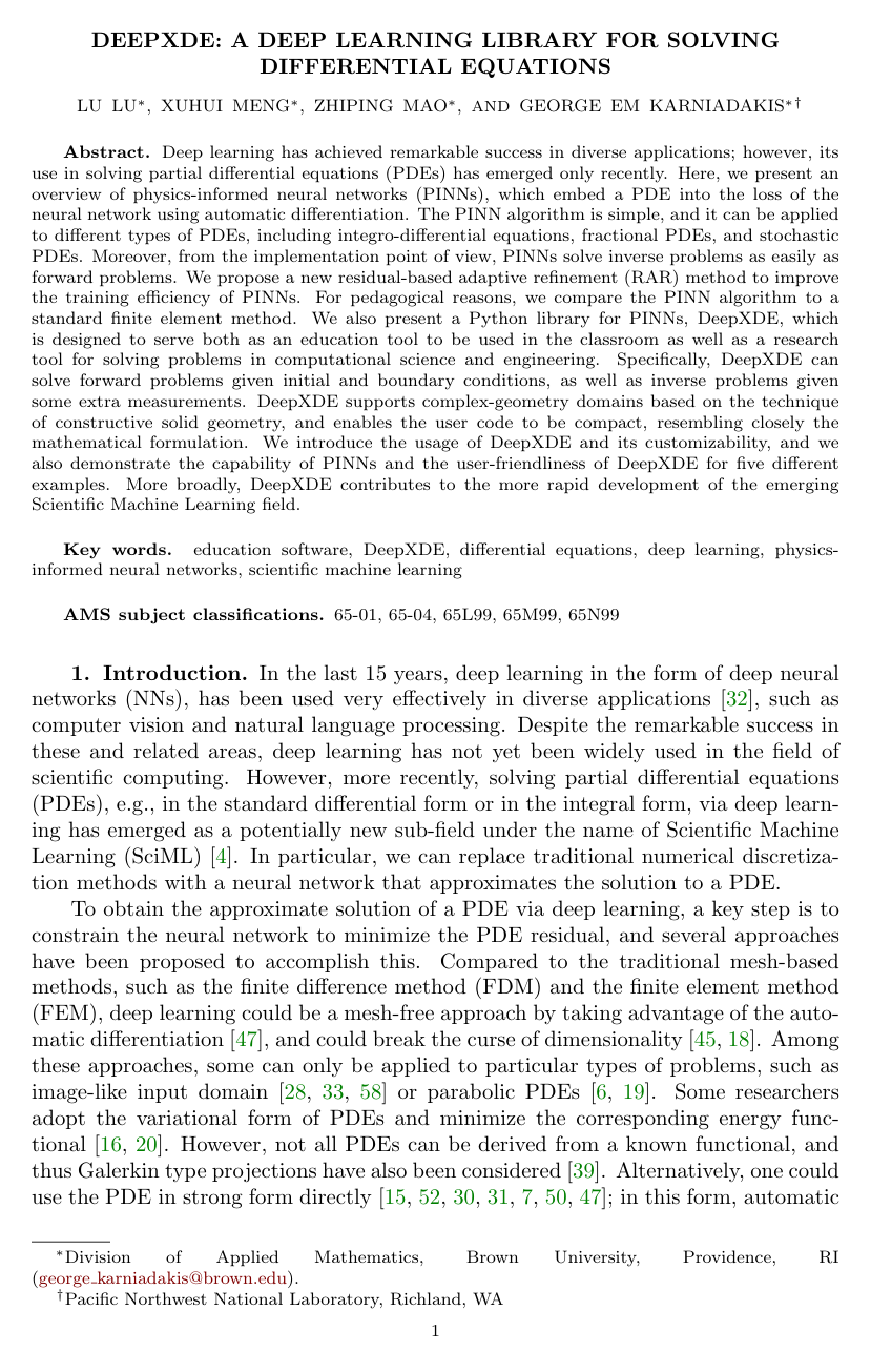
Cover for DeepXDE: A Deep Learning Library for Solving Differential Equations

Abstract

Deep learning has achieved remarkable success in diverse applications; however, its use in solving partial differential equations (PDEs) has emerged only recently. Here, we present an overview of physics-informed neural networks (PINNs), which embed a PDE into the loss of the neural network using automatic differentiation. The PINN algorithm is simple, and it can be applied to different types of PDEs, including integro-differential equations, fractional PDEs, and stochastic PDEs. Moreover, from the implementation point of view, PINNs solve inverse problems as easily as forward problems. We propose a new residual-based adaptive refinement (RAR) method to improve the training efficiency of PINNs. For pedagogical reasons, we compare the PINN algorithm to a standard finite element method. We also present a Python library for PINNs, DeepXDE, which is designed to serve both as an education tool to be used in the classroom as well as a research tool for solving problems in computational science and engineering. Specifically, DeepXDE can solve forward problems given initial and boundary conditions, as well as inverse problems given some extra measurements. DeepXDE supports complex-geometry domains based on the technique of constructive solid geometry, and enables the user code to be compact, resembling closely the mathematical formulation. We introduce the usage of DeepXDE and its customizability, and we also demonstrate the capability of PINNs and the user-friendliness of DeepXDE for five different examples. More broadly, DeepXDE contributes to the more rapid development of the emerging Scientific Machine Learning field.

Table of Contents

  • 1 Introduction
  • 2 Algorithm and theory of physics-informed neural networks
  • 2.1 Deep neural networks
  • 2.2 Automatic differentiation
  • 2.3 Physics-informed neural networks (PINNs) for solving PDEs
  • 2.4 Approximation theory and error analysis for PINNs
  • 2.5 Comparison between PINNs and FEM
  • 2.6 PINNs for solving integro-differential equations
  • 2.7 PINNs for solving inverse problems
  • 2.8 Residual-based adaptive refinement (RAR)
  • 3 DeepXDE usage and customization
  • 3.1 Usage
  • 3.2 Customizability
  • 3.2.1 Geometry
  • 3.2.2 Neural networks
  • 3.2.3 Callbacks
  • 4 Demonstration examples
  • 4.1 Poisson equation over an L-shaped domain
  • 4.2 RAR for Burgers equation
  • 4.3 Inverse problem for the Lorenz system
  • 4.4 Inverse problem for diffusion-reaction systems
  • 4.5 Volterra IDE
  • 5 Concluding Remarks
  • References

Knowls

  1. Knowl 1 — Residual-Based Adaptive Refinement Algorithm

    algorithm

    The Residual-Based Adaptive Refinement (RAR) method dynamically enriches the set of collocation (residual) points during physics-informed neural network (PINN) training by placing new points in regions with large PDE residuals.

    Input: Initial residual points T\mathcal{T}, candidate pool sample size S|\mathcal{S}|, number of points to add per step mm, mean residual stopping threshold E0\mathcal{E}_0
    Output: Trained neural network parameters θ\theta^* and refined training set T\mathcal{T}
    Train the neural network u^(x;θ)\hat{u}(\mathbf{x}; \theta) on T\mathcal{T} for a limited number of iterations
    repeat
        Sample a random set of locations S={x1,x2,,xS}Ω\mathcal{S} = \{\mathbf{x}_1, \mathbf{x}_2, \dots, \mathbf{x}_{|\mathcal{S}|}\} \subset \Omega
        Estimate mean PDE residual:
            Er1SxSf(x;u^x1,,2u^x12,;λ)\mathcal{E}_r \leftarrow \frac{1}{|\mathcal{S}|} \sum_{\mathbf{x} \in \mathcal{S}} \left\| f\left(\mathbf{x}; \frac{\partial \hat{u}}{\partial x_1}, \dots, \frac{\partial^2 \hat{u}}{\partial x_1^2}, \dots; \lambda\right) \right\|
        if Er<E0\mathcal{E}_r < \mathcal{E}_0 then
            break
        end if
        Identify the mm points in S\mathcal{S} with the highest residual norms
        TT{m selected points}\mathcal{T} \leftarrow \mathcal{T} \cup \{m \text{ selected points}\}
        Train the neural network u^(x;θ)\hat{u}(\mathbf{x}; \theta) on updated T\mathcal{T} for a limited number of iterations
    until converged
    return θ,T\theta^*, \mathcal{T}

    Here, f(x;;λ)=0f(\mathbf{x}; \dots; \lambda) = 0 denotes the parameterized PDE operator over domain ΩRd\Omega \subset \mathbb{R}^d with volume VV, and Er\mathcal{E}_r provides a Monte Carlo estimate of the mean residual 1VΩf(x;;λ)dx\frac{1}{V} \int_\Omega \|f(\mathbf{x}; \dots; \lambda)\| d\mathbf{x}.

  2. Knowl 2 — PINN Loss Formulation for Forward and Inverse PDE Problems

    model/method

    A Physics-Informed Neural Network (PINN) approximates the solution u(x)u(\mathbf{x}) of a general partial differential equation parameterized by λ\lambda on a domain ΩRd\Omega \subset \mathbb{R}^d:

    f(x;ux1,,uxd;2ux1x1,;λ)=0,xΩf\left(\mathbf{x}; \frac{\partial u}{\partial x_1}, \dots, \frac{\partial u}{\partial x_d}; \frac{\partial^2 u}{\partial x_1 \partial x_1}, \dots; \lambda\right) = 0, \quad \mathbf{x} \in \Omega

    subject to boundary and initial conditions B(u,x)=0\mathcal{B}(u, \mathbf{x}) = 0 on Ω\partial \Omega. For time-dependent problems, time tt is incorporated as a component of x\mathbf{x}, and initial conditions are treated as Dirichlet boundary conditions on the spatio-temporal boundary.

    A neural network surrogate u^(x;θ)\hat{u}(\mathbf{x}; \theta) with parameters θ={W,b}=1L\theta = \{W^\ell, b^\ell\}_{\ell=1}^L is trained by minimizing the composite loss:

    L(θ,λ;T)=wfLf(θ,λ;Tf)+wbLb(θ,λ;Tb)+wiLi(θ,λ;Ti)\mathcal{L}(\theta, \lambda; \mathcal{T}) = w_f \mathcal{L}_f(\theta, \lambda; \mathcal{T}_f) + w_b \mathcal{L}_b(\theta, \lambda; \mathcal{T}_b) + w_i \mathcal{L}_i(\theta, \lambda; \mathcal{T}_i)

    where wf,wb,wiw_f, w_b, w_i are positive weight coefficients, and the component residuals are given by:

    Lf(θ,λ;Tf)=1TfxTff(x;u^x1,,2u^x12,;λ)2\mathcal{L}_f(\theta, \lambda; \mathcal{T}_f) = \frac{1}{|\mathcal{T}_f|} \sum_{\mathbf{x} \in \mathcal{T}_f} \left\| f\left(\mathbf{x}; \frac{\partial \hat{u}}{\partial x_1}, \dots, \frac{\partial^2 \hat{u}}{\partial x_1^2}, \dots; \lambda\right) \right\|^2

    Lb(θ,λ;Tb)=1TbxTbB(u^,x)2\mathcal{L}_b(\theta, \lambda; \mathcal{T}_b) = \frac{1}{|\mathcal{T}_b|} \sum_{\mathbf{x} \in \mathcal{T}_b} \|\mathcal{B}(\hat{u}, \mathbf{x})\|^2

    Li(θ,λ;Ti)=1TixTiI(u^,x)2\mathcal{L}_i(\theta, \lambda; \mathcal{T}_i) = \frac{1}{|\mathcal{T}_i|} \sum_{\mathbf{x} \in \mathcal{T}_i} \|\mathcal{I}(\hat{u}, \mathbf{x})\|^2

    Here, TfΩ\mathcal{T}_f \subset \Omega is the set of interior residual collocation points, TbΩ\mathcal{T}_b \subset \partial\Omega is the boundary/initial point set, and TiΩ\mathcal{T}_i \subset \Omega is the set of observation points where extra measurements I(u,x)=0\mathcal{I}(u, \mathbf{x}) = 0 are available. All required derivatives with respect to inputs x\mathbf{x} are computed via automatic differentiation (AD). For forward problems, λ\lambda is fixed and optimization is performed over θ\theta. For inverse problems, optimization is conducted jointly over θ\theta and the unknown parameters λ\lambda.

  3. Knowl 3 — Error Decomposition of Physics-Informed Neural Networks

    theoretical result

    Let uu be the exact solution of a PDE, and let F\mathcal{F} denote the family of functions realizable by a chosen neural network architecture. Let uF=argminfFfuu_\mathcal{F} = \arg\min_{f \in \mathcal{F}} \|f - u\| be the best approximation to uu in F\mathcal{F}, let uT=argminfFL(f;T)u_\mathcal{T} = \arg\min_{f \in \mathcal{F}} \mathcal{L}(f; \mathcal{T}) denote the global minimizer of the training loss over collocation set T\mathcal{T}, and let u~T\tilde{u}_\mathcal{T} be the numerical solution obtained after optimization.

    The total error E:=u~Tu\mathcal{E} := \|\tilde{u}_\mathcal{T} - u\| is upper-bounded by the sum of optimization, generalization, and approximation errors:

    EEopt+Egen+Eapp\mathcal{E} \le \mathcal{E}_{\text{opt}} + \mathcal{E}_{\text{gen}} + \mathcal{E}_{\text{app}}

    where:

    1. Optimization error: Eopt=u~TuT\mathcal{E}_{\text{opt}} = \|\tilde{u}_\mathcal{T} - u_\mathcal{T}\|, arising from optimization failure to find the global minimum due to loss landscape non-convexity, learning rate, and finite training steps.
    2. Generalization error: Egen=uTuF\mathcal{E}_{\text{gen}} = \|u_\mathcal{T} - u_\mathcal{F}\|, determined by the finite number and spatial distribution of the training collocation points in T\mathcal{T}.
    3. Approximation error: Eapp=uFu\mathcal{E}_{\text{app}} = \|u_\mathcal{F} - u\|, determined by the expressivity and capacity of the neural network space F\mathcal{F}.
  4. Knowl 4 — Simultaneous Frequency Learning Dynamics in PINNs

    empirical result

    While deep neural networks applied to standard function fitting exhibit spectral bias (the Frequency Principle), learning low-frequency components before high-frequency components, PINNs learn all Fourier frequency modes nearly simultaneously.

    When fitting the target multi-frequency function f(x)=k=15sin(2kx)2kf(x) = \sum_{k=1}^5 \frac{\sin(2kx)}{2k} on [π,π][-\pi, \pi] directly with a 4-hidden-layer, 20-neurons-per-layer feed-forward network (learning rate 10410^{-4}, 500 random points), low frequencies (k=1,2k=1, 2) converge significantly earlier than high frequencies (k=4,5k=4, 5).

    In contrast, when training a PINN of identical architecture to solve the corresponding Poisson boundary value problem:

    fxx=k=152ksin(2kx),x[π,π],f(π)=f(π)=0-f_{xx} = \sum_{k=1}^5 2k \sin(2kx), \quad x \in [-\pi, \pi], \quad f(-\pi) = f(\pi) = 0

    the presence of the differential operator causes the network to learn all five frequency modes at approximately the same rate across training iterations, leading to faster overall convergence than direct function regression.

  5. Knowl 5 — PINN Formulation for Integro-Differential Equations

    model/method

    Physics-informed neural networks solve integro-differential equations (IDEs) by combining automatic differentiation for differential operators with numerical quadrature schemes for integral operators.

    For a Volterra integro-differential equation of the form:

    dydx+y(x)=0xetxy(t)dt\frac{dy}{dx} + y(x) = \int_0^x e^{t-x} y(t) dt

    the integral operator is approximated via nn-point numerical quadrature:

    0xetxy(t)dti=1nwieti(x)xy(ti(x))\int_0^x e^{t-x} y(t) dt \approx \sum_{i=1}^n w_i e^{t_i(x) - x} y(t_i(x))

    where {wi}i=1n\{w_i\}_{i=1}^n and {ti(x)}i=1n\{t_i(x)\}_{i=1}^n are quadrature weights and abscissae mapped to [0,x][0, x]. The PINN surrogate y^(x;θ)\hat{y}(x; \theta) minimizes the surrogate PDE residual:

    Lf(θ;Tf)=1TfxTf(dy^dx(x)+y^(x)i=1nwieti(x)xy^(ti(x)))2\mathcal{L}_f(\theta; \mathcal{T}_f) = \frac{1}{|\mathcal{T}_f|} \sum_{x \in \mathcal{T}_f} \left( \frac{d\hat{y}}{dx}(x) + \hat{y}(x) - \sum_{i=1}^n w_i e^{t_i(x) - x} \hat{y}(t_i(x)) \right)^2

    where dy^dx\frac{d\hat{y}}{dx} is computed via automatic differentiation. This introduces a fourth error term, the discretization error Edis\mathcal{E}_{\text{dis}}, alongside approximation, generalization, and optimization errors.

  6. Knowl 6 — Constructive Solid Geometry Domain Modeling in DeepXDE

    model/method

    DeepXDE implements constructive solid geometry (CSG) to construct complex 2D and 3D computational domains without traditional mesh generation. Built-in primitive geometries include interval, triangle, rectangle, polygon, disk, cuboid, and sphere.

    Arbitrary complex geometries are formed through boolean operations between geometry objects:

    1. Union: geom1 | geom2
    2. Difference: geom1 - geom2
    3. Intersection: geom1 & geom2

    Each geometry object provides core methods for point containment (inside(x)), boundary evaluation (on_boundary(x)), normal vector calculation (boundary_normal(x) for Neumann and Robin conditions), periodic mapping (periodic_point(x, component)), and uniform or pseudo-random point sampling (random_points(n), random_boundary_points(n)).

  7. Knowl 7 — Structural Comparison Between PINNs and the Finite Element Method

    data/table

    Physics-informed neural networks and the Finite Element Method (FEM) compare across core mathematical and computational characteristics as follows:

    Feature PINN FEM
    Basis function Neural network (nonlinear) Piecewise polynomial (linear)
    Parameters Weights and biases Point values
    Training points Scattered points (mesh-free) Mesh points
    PDE embedding Loss function Algebraic system
    Parameter solver Gradient-based optimizer Linear solver
    Errors Eapp,Egen,Eopt\mathcal{E}_{\text{app}}, \mathcal{E}_{\text{gen}}, \mathcal{E}_{\text{opt}} Approximation and quadrature errors
    Error bounds Not available Partially available

    Unlike FEM, which linearizes the solution via piecewise polynomials over generated meshes and solves an exact linear system (using stiffness and mass matrices), PINNs perform nonlinear optimization using gradient-based algorithms (such as Adam and L-BFGS) over mesh-free scattered collocation points by embedding the strong form of the differential equation and boundary conditions directly into the objective function.

  8. Knowl 8 — Empirical Performance of RAR on 1D and 2D Burgers Equations

    empirical result

    Residual-Based Adaptive Refinement (RAR) was evaluated on both 1D and 2D Burgers equations to assess its capability in resolving steep gradients and discontinuities:

    1. 1D Viscous Burgers Equation: tu+uxu=νxxu\partial_t u + u \partial_x u = \nu \partial_{xx} u on x[1,1],t[0,1]x \in [-1, 1], t \in [0, 1] with ν=0.01/π\nu = 0.01/\pi, initial condition u(x,0)=sin(πx)u(x, 0) = -\sin(\pi x), and zero Dirichlet boundary conditions. Initialized with 2500 random spatio-temporal residual points, RAR iteratively added m=1m=1 point per cycle until reaching 2540 points (threshold E0=0.005\mathcal{E}_0 = 0.005). The added points concentrated precisely along the sharp shock front at x=0x = 0. PINN with RAR reduced the L2L^2 relative error and eliminated oscillatory shock artifacts compared to standard PINN trained on 2540 uniformly sampled points and coarse finite difference simulations (2400 points).

    2. 2D Viscous Burgers Equation: Coupled system for velocities u,vu, v at Reynolds number Re=5000\text{Re} = 5000 on [0,1]2×[0,1][0, 1]^2 \times [0, 1]. Starting with 200 spatio-temporal residual points (plus 5000 initial and 1000 boundary points), RAR added only 10 adaptive residual points (total 210 points). The resulting PINN profile at y=2/3y=2/3 accurately captured the steep moving shock wave across t{0.2,0.5,1.0}t \in \{0.2, 0.5, 1.0\}, whereas a PINN with 210 non-adaptive random points failed to resolve the sharp transition.

  9. Knowl 9 — Inverse Parameter Identification in Chaotic and Reaction-Diffusion Systems

    empirical result

    PINNs implemented in DeepXDE accurately infer unknown physical parameters from sparse observation data:

    1. Lorenz System: Defined by dxdt=ρ(yx)\frac{dx}{dt} = \rho(y - x), dydt=x(σz)y\frac{dy}{dt} = x(\sigma - z) - y, dzdt=xyβz\frac{dz}{dt} = xy - \beta z with true parameters (ρ,σ,β)=(10,15,8/32.6667)(\rho, \sigma, \beta) = (10, 15, 8/3 \approx 2.6667). Given initial conditions (8,7,27)(-8, 7, 27), 400 interior collocation points Tf\mathcal{T}_f, and only 25 observation points Ti\mathcal{T}_i over t[0,3]t \in [0, 3], PINN identified parameters as (ρ,σ,β)=(10.002,14.999,2.668)(\rho, \sigma, \beta) = (10.002, 14.999, 2.668) within 60,000 Adam iterations.

    2. Porous Media Diffusion-Reaction System: Solute concentrations CA,CBC_A, C_B undergoing A+2BCA + 2B \to C governed by tCA=DxxCAkfCACB2\partial_t C_A = D \partial_{xx} C_A - k_f C_A C_B^2 and tCB=DxxCB2kfCACB2\partial_t C_B = D \partial_{xx} C_B - 2 k_f C_A C_B^2 on x[0,1],t[0,10]x \in [0, 1], t \in [0, 10] with true effective diffusion coefficient D=2×10³D = 2 \times 10^{-3} and reaction rate kf=0.1k_f = 0.1. From 40,000 spatio-temporal observations, the PINN simultaneously converged to estimated values D=1.98×10³D = 1.98 \times 10^{-3} and kf=0.0971k_f = 0.0971 within 80,000 Adam iterations.

  10. Knowl 10 — Limitations of Physics-Informed Neural Networks

    limitation

    PINNs present several structural and computational limitations:

    1. Computational Speed for Forward Problems: For standard forward PDE simulations, PINNs are computationally slower than classical finite element methods due to the cost of iterative non-convex gradient optimization and high-order automatic differentiation.
    2. Optimization and Convergence: Training PINNs involves solving non-convex optimization problems with no guarantee of convergence to the global minimum or unique solutions; networks initialized from different random seeds may converge to distinct local minima.
    3. Network Architecture Selection: Choosing optimal network depth, width, and activation functions remains empirical and problem-dependent, requiring manual tuning or meta-learning.
    4. Long Time Integration: Standard spatio-temporal PINN training struggles over long temporal horizons without time-parallel decomposition or domain decomposition methods.
    5. Curvilinear Geometry Accuracy: Enforcing exact boundary conditions on complex curvilinear geometries without spline-based representations (such as NURBS) remains challenging.

Coverage note — None was omitted; all key theoretical formulations, the novel RAR algorithm, software abstractions (CSG/DeepXDE workflow), error analyses, and numerical forward/inverse benchmark cases have been captured.

References

  1. 1.M. Abadi, P. Barham, J. Chen, Z. Chen, A. Davis, J. Dean, M. Devin, S. Ghemawat, G. Irving, M. Isard, et al., Tensorflow: A system for large-scale machine learning, in 12th USENIX Symposium on Operating Systems Design and Implementation, 2016, pp. 265–283.
  2. 2.M. Ainsworth and J. T. Oden, A posteriori error estimation in finite element analysis, vol. 37, John Wiley & Sons, 2011.
  3. 3.A. Baeza and P. Mulet, Adaptive mesh refinement techniques for high-order shock capturing schemes for multi-dimensional hydrodynamic simulations, International Journal for Numerical Methods in Fluids, 52 (2006), pp. 455–471.
  4. 4.N. Baker, F. Alexander, T. Bremer, A. Hagberg, Y. Kevrekidis, H. Najm, M. Parashar, A. Patra, J. Sethian, S. Wild, et al., Workshop report on basic research needs for scientific machine learning: Core technologies for artificial intelligence, tech. report, US DOE Office of Science, Washington, DC (United States), 2019.
  5. 5.A. G. Baydin, B. A. Pearlmutter, A. A. Radul, and J. M. Siskind, Automatic differentiation in machine learning: a survey, The Journal of Machine Learning Research, 18 (2017), pp. 5595–5637.
  6. 6.C. Beck, W. E, and A. Jentzen, Machine learning approximation algorithms for high-dimensional fully nonlinear partial differential equations and second-order backward stochastic differential equations, Journal of Nonlinear Science, (2017), pp. 1–57.
  7. 7.J. Berg and K. Nyström, A unified deep artificial neural network approach to partial differential equations in complex geometries, Neurocomputing, 317 (2018), pp. 28–41.
  8. 8.M. Betancourt, A geometric theory of higher-order automatic differentiation, arXiv preprint arXiv:1812.11592, (2018).
  9. 9.J. Bettencourt, M. J. Johnson, and D. Duvenaud, Taylor-mode automatic differentiation for higher-order derivatives in jax, (2019).
  10. 10.A. Blum and R. L. Rivest, Training a 3-node neural network is np-complete, in Advances in Neural Information Processing Systems, 1989, pp. 494–501.
  11. 11.L. Bottou and O. Bousquet, The tradeoffs of large scale learning, in Advances in Neural Information Processing Systems, 2008, pp. 161–168.
  12. 12.R. H. Byrd, P. Lu, J. Nocedal, and C. Zhu, A limited memory algorithm for bound constrained optimization, SIAM Journal on Scientific Computing, 16 (1995), pp. 1190–1208.
  13. 13.Y. Chen, L. Lu, G. E. Karniadakis, and L. D. Negro, Physics-informed neural networks for inverse problems in nano-optics and metamaterials, arXiv preprint arXiv:1912.01085, (2019).
  14. 14.P. G. Ciarlet, The finite element method for elliptic problems, vol. 40, Siam, 2002.
  15. 15.M. Dissanayake and N. Phan-Thien, Neural-network-based approximations for solving partial differential equations, Communications in Numerical Methods in Engineering, 10 (1994), pp. 195–201.
  16. 16.W. E and B. Yu, The deep Ritz method: A deep learning-based numerical algorithm for solving variational problems, Communications in Mathematics and Statistics, 6 (2018), pp. 1–12.
  17. 17.C. Finn, P. Abbeel, and S. Levine, Model-agnostic meta-learning for fast adaptation of deep networks, in Proceedings of the 34th International Conference on Machine Learning, 2017, pp. 1126–1135.
  18. 18.P. Grohs, F. Hornung, A. Jentzen, and P. Von Wurstemberger, A proof that artificial neural networks overcome the curse of dimensionality in the numerical approximation of black-scholes partial differential equations, arXiv preprint arXiv:1809.02362, (2018).
  19. 19.J. Han, A. Jentzen, and W. E, Solving high-dimensional partial differential equations using deep learning, Proceedings of the National Academy of Sciences, 115 (2018), pp. 8505–8510.
  20. 20.J. He, L. Li, J. Xu, and C. Zheng, ReLU deep neural networks and linear finite elements, arXiv preprint arXiv:1807.03973, (2018).
  21. 21.Q. He, D. Brajas-Solano, G. Tartakovsky, and A. M. Tartakovsky, Physics-informed neural networks for multiphysics data assimilation with application to subsurface transport, arXiv preprint arXiv:1912.02968, (2019).
  22. 22.T. J. Hughes, J. A. Cottrell, and Y. Bazilevs, Isogeometric analysis: Cad, finite elements, nurbs, exact geometry and mesh refinement, Computer methods in applied mechanics and engineering, 194 (2005), pp. 4135–4195.
  23. 23.A. D. Jagtap, K. Kawaguchi, and G. E. Karniadakis, Locally adaptive activation functions with slope recovery term for deep and physics-informed neural networks, arXiv preprint arXiv:1909.12228, (2019).
  24. 24.A. D. Jagtap, K. Kawaguchi, and G. E. Karniadakis, Adaptive activation functions accelerate convergence in deep and physics-informed neural networks, Journal of Computational Physics, 404 (2020), p. 109136.
  25. 25.P. Jin, L. Lu, Y. Tang, and G. E. Karniadakis, Quantifying the generalization error in deep learning in terms of data distribution and neural network smoothness, arXiv preprint arXiv:1905.11427, (2019).
  26. 26.C. Johnson, Numerical solution of partial differential equations by the finite element method, Courier Corporation, 2012.
  27. 27.G. E. Karniadakis and S. J. Sherwin, Spectral/hp element methods for computational fluid dynamics, Oxford University Press, second ed., 2013.
  28. 28.Y. Khoo, J. Lu, and L. Ying, Solving parametric PDE problems with artificial neural networks, arXiv preprint arXiv:1707.03351, (2017).
  29. 29.D. P. Kingma and J. Ba, Adam: A method for stochastic optimization, in International Conference on Learning Representations, 2015.
  30. 30.I. E. Lagaris, A. Likas, and D. I. Fotiadis, Artificial neural networks for solving ordinary and partial differential equations, IEEE Transactions on Neural Networks, 9 (1998), pp. 987–1000.
  31. 31.I. E. Lagaris, A. C. Likas, and D. G. Papageorgiou, Neural-network methods for boundary value problems with irregular boundaries, IEEE Transactions on Neural Networks, 11 (2000), pp. 1041–1049.
  32. 32.Y. LeCun, Y. Bengio, and G. Hinton, Deep learning, Nature, 521 (2015), p. 436.
  33. 33.Z. Long, Y. Lu, X. Ma, and B. Dong, PDE-net: Learning PDEs from data, in International Conference on Machine Learning, 2018, pp. 3214–3222.
  34. 34.L. Lu, P. Jin, and G. E. Karniadakis, DeepONet: Learning nonlinear operators for identifying differential equations based on the universal approximation theorem of operators, arXiv preprint arXiv:1910.03193, (2019).
  35. 35.L. Lu, Y. Shin, Y. Su, and G. E. Karniadakis, Dying ReLU and initialization: Theory and numerical examples, arXiv preprint arXiv:1903.06733, (2019).
  36. 36.L. Lu, Y. Su, and G. E. Karniadakis, Collapse of deep and narrow neural nets, arXiv preprint arXiv:1808.04947, (2018).
  37. 37.Z. Mao, A. D. Jagtap, and G. E. Karniadakis, Physics-informed neural networks for high-speed flows, Computer Methods in Applied Mechanics and Engineering, 360 (2020), p. 112789.
  38. 38.C. C. Margossian, A review of automatic differentiation and its efficient implementation, Wiley Interdisciplinary Reviews: Data Mining and Knowledge Discovery, 9 (2019), p. e1305.
  39. 39.A. J. Meade Jr and A. A. Fernandez, The numerical solution of linear ordinary differential equations by feedforward neural networks, Mathematical and Computer Modelling, 19 (1994), pp. 1–25.
  40. 40.X. Meng and G. E. Karniadakis, A composite neural network that learns from multi-fidelity data: Application to function approximation and inverse PDE problems, arXiv preprint arXiv:1903.00104, (2019).
  41. 41.M. A. Nabian and H. Meidani, A deep neural network surrogate for high-dimensional random partial differential equations, arXiv preprint arXiv:1806.02957, (2018).
  42. 42.G. Pang, L. Lu, and G. E. Karniadakis, fPINNs: Fractional physics-informed neural networks, SIAM Journal on Scientific Computing, 41 (2019), pp. A2603–A2626.
  43. 43.A. Paszke, S. Gross, S. Chintala, G. Chanan, E. Yang, Z. DeVito, Z. Lin, A. Desmaison, L. Antiga, and A. Lerer, Automatic differentiation in PyTorch, (2017).
  44. 44.A. Pinkus, Approximation theory of the MLP model in neural networks, Acta Numerica, 8 (1999), pp. 143–195.
  45. 45.T. Poggio, H. Mhaskar, L. Rosasco, B. Miranda, and Q. Liao, Why and when can deep-but not shallow-networks avoid the curse of dimensionality: a review, International Journal of Automation and Computing, 14 (2017), pp. 503–519.
  46. 46.N. Rahaman, A. Baratin, D. Arpit, F. Draxler, M. Lin, F. Hamprecht, Y. Bengio, and A. Courville, On the spectral bias of neural networks, in Proceedings of the 36th International Conference on Machine Learning, 2019, pp. 5301–5310.
  47. 47.M. Raissi, P. Perdikaris, and G. E. Karniadakis, Physics-informed neural networks: A deep learning framework for solving forward and inverse problems involving nonlinear partial differential equations, Journal of Computational Physics, 378 (2019), pp. 686–707.
  48. 48.M. Raissi, A. Yazdani, and G. E. Karniadakis, Hidden fluid mechanics: Learning velocity and pressure fields from flow visualizations, Science, (2020).
  49. 49.D. E. Rumelhart, G. E. Hinton, and R. J. Williams, Learning representations by back-propagating errors, Nature, 323 (1986), pp. 533–536.
  50. 50.J. Sirignano and K. Spiliopoulos, DGM: A deep learning algorithm for solving partial differential equations, Journal of Computational Physics, 375 (2018), pp. 1339–1364.
  51. 51.A. M. Tartakovsky, C. O. Marrero, P. Perdikaris, G. D. Tartakovsky, and D. Barajas-Solano, Learning parameters and constitutive relationships with physics informed deep neural networks, arXiv preprint arXiv:1808.03398, (2018).
  52. 52.B. P. van Milligen, V. Tribaldos, and J. Jiménez, Neural network differential equation and plasma equilibrium solver, Physical Review Letters, 75 (1995), p. 3594.
  53. 53.N. Winovich, K. Ramani, and G. Lin, ConvPDE-UQ: Convolutional neural networks with quantified uncertainty for heterogeneous elliptic partial differential equations on varied domains, Journal of Computational Physics, 394 (2019), pp. 263–279.
  54. 54.Z.-Q. J. Xu, Y. Zhang, T. Luo, Y. Xiao, and Z. Ma, Frequency principle: Fourier analysis sheds light on deep neural networks, arXiv preprint arXiv:1901.06523, (2019).
  55. 55.L. Yang, D. Zhang, and G. E. Karniadakis, Physics-informed generative adversarial networks for stochastic differential equations, arXiv preprint arXiv:1811.02033, (2018).
  56. 56.D. Zhang, L. Guo, and G. E. Karniadakis, Learning in modal space: Solving time-dependent stochastic PDEs using physics-informed neural networks, arXiv preprint arXiv:1905.01205, (2019).
  57. 57.D. Zhang, L. Lu, L. Guo, and G. E. Karniadakis, Quantifying total uncertainty in physics-informed neural networks for solving forward and inverse stochastic problems, Journal of Computational Physics, 397 (2019), p. 108850.
  58. 58.Y. Zhu, N. Zabaras, P.-S. Koutsourelakis, and P. Perdikaris, Physics-constrained deep learning for high-dimensional surrogate modeling and uncertainty quantification without labeled data, arXiv preprint arXiv:1901.06314, (2019).
  59. 59.B. Zoph and Q. V. Le, Neural architecture search with reinforcement learning, arXiv preprint arXiv:1611.01578, (2016).

Citation

MLA
Lu, L., et al. “DeepXDE: A Deep Learning Library for Solving Differential Equations”. SIAM Review, vol. 63, no. 1, 2021, pp. 208–28, https://doi.org/10.1137/19M1274067.
APA
Lu, L., Meng, X., Mao, Z., & Karniadakis, G. E. (2021). DeepXDE: A Deep Learning Library for Solving Differential Equations. SIAM Review, 63(1), 208–228. https://doi.org/10.1137/19M1274067
Chicago
Lu, L., X. Meng, Z. Mao, and G. E. Karniadakis. 2021. “DeepXDE: A Deep Learning Library for Solving Differential Equations”. SIAM Review 63 (1): 208–28. https://doi.org/10.1137/19M1274067.
Harvard
Lu, L. et al. (2021) “DeepXDE: A Deep Learning Library for Solving Differential Equations”, SIAM Review, 63(1), pp. 208–228. Available at: https://doi.org/10.1137/19M1274067.
Vancouver
1. Lu L, Meng X, Mao Z, Karniadakis GE (2021) DeepXDE: A Deep Learning Library for Solving Differential Equations. SIAM Review 63:208–228

BibTeX

@article{Lu_2021, title={DeepXDE: A Deep Learning Library for Solving Differential Equations}, volume={63}, ISSN={1095-7200}, url={http://dx.doi.org/10.1137/19M1274067}, DOI={10.1137/19m1274067}, number={1}, journal={SIAM Review}, publisher={Society for Industrial & Applied Mathematics (SIAM)}, author={Lu, Lu and Meng, Xuhui and Mao, Zhiping and Karniadakis, George Em}, year={2021}, month=Jan, pages={208–228} }
Metadata:Crossref

Source Code

This paper has an official code repository available. Click below to access the source code.

View Repository

Access the Paper

This paper is available from its original source. Click below to access the PDF.

Open PDF