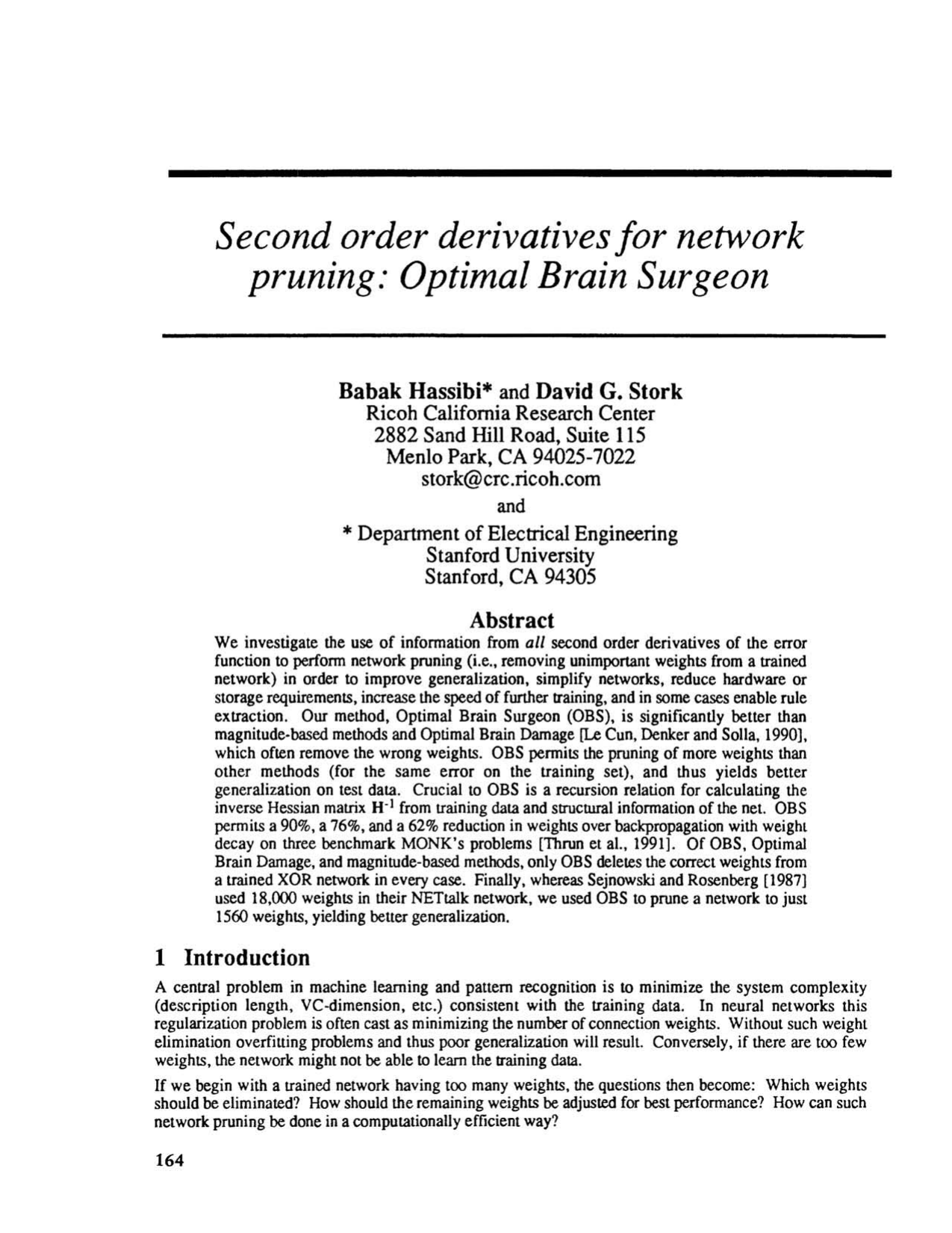
Second Order Derivatives for Network Pruning: Optimal Brain Surgeon

Babak HassibiDavid G. Stork

article1992NeurIPS2,181 citations

Introduces Optimal Brain Surgeon, a pruning framework that leverages the full inverse Hessian matrix to accurately identify redundant weights and automatically compensate remaining parameters without retraining, outperforming diagonal approximations and magnitude-based methods.

Listen

Artificial neural networks often suffer from overfitting and poor generalization when configured with too many connection parameters, while also requiring excessive computing hardware and storage. Existing methods for pruning unnecessary connections either delete weights based solely on their small size or rely on restrictive mathematical simplifications, frequently removing critical parameters and permanently harming model performance.

The article introduces and evaluates Optimal Brain Surgeon, an advanced pruning method that utilizes full second-order error curvature to identify unimportant connections and automatically update all remaining parameters without requiring retraining.

The researchers developed a recursive formula that calculates the full error curvature across a single sequential pass over the training data, avoiding complex matrix inversions. They evaluated the approach across standard logical benchmarks, including the XOR and MONK's problems, as well as a large-scale real-world speech synthesis task (NETtalk).

The analysis yielded several key findings regarding model efficiency and accuracy. First, the method consistently identified the correct parameters to delete in the XOR test, whereas traditional magnitude-based and simplified curvature methods removed incorrect parameters that could not be corrected even with subsequent retraining. Second, across three benchmark MONK's problems, the method reduced the required connection weights by 76%, 62%, and 90% compared to standard regularization techniques, while maintaining 100% test accuracy on the first two tasks and matching baseline accuracy on the third. Third, applying the technique to the NETtalk speech synthesis system pruned the architecture down to 1,560 weights—compared to the 18,000 weights in original implementations—while reducing test error from 5,259 to 4,701.

These findings demonstrate that retaining full error curvature information allows organizations to drastically streamline neural networks without sacrificing accuracy. Reducing model sizes by over 60% to 90% cuts operational memory footprints and computational costs, accelerates deployment speeds, and simplifies network structures sufficiently to enable the extraction of human-interpretable logical rules.

Decision-makers and engineering teams should consider adopting this pruning approach for production-level artificial intelligence models in domains like speech recognition and optical character recognition. The method can be combined directly with existing techniques, such as weight decay during initial training, though practitioners must establish problem-specific stopping criteria to determine when further pruning degrades overall performance.

Confidence in these findings is high for fully trained networks reaching local error minima. However, the technique relies on the mathematical assumption that higher-order error terms above the second derivative are negligible near convergence, meaning practitioners should exercise caution and validate performance if attempting to prune models that are severely undertrained.

Department of Electrical Engineering Ricoh California Research Center Stanford University backpropagation network computer hardware training sample Optimal Brain Surgeon network pruning second order derivatives

Hassibi et al (1992).pdf

Paper: Optimal Brain Damage, Yann LeCun et al. (1989). Introduces the foundational second-order Taylor expansion framework for weight saliency (Optimal Brain Damage) that Optimal Brain Surgeon directly critiques, improves, and generalizes by incorporating off-diagonal Hessian terms.
Paper: A Simple Weight Decay Can Improve Generalization, Anders Krogh et al. (1991). Provides the theoretical and empirical baseline for weight decay regularization that Optimal Brain Surgeon explicitly benchmarks against and outperforms on standard tasks.

Paper: Pruning Convolutional Neural Networks for Resource Efficient Inference, Pavlo Molchanov et al. (2016). Extends Taylor-expansion-based pruning criteria to structured filter and feature-map removal in modern deep convolutional networks.
Paper: Learning both Weights and Connections for Efficient Neural Networks, Song Han et al. (2015). Revisits iterative weight pruning and retraining pipelines to dramatically compress large deep neural network architectures.
Paper: Deep Compression: Compressing Deep Neural Network with Pruning, Trained Quantization and Huffman Coding, Song Han et al. (2015). Builds on iterative network pruning methods by combining them with weight quantization and Huffman coding for end-to-end model compression.
Paper: The Lottery Ticket Hypothesis: Finding Sparse, Trainable Neural Networks., Jonathan Frankle et al. (2019). Investigates the sparse subnetworks uncovered by pruning algorithms to formulate the Lottery Ticket Hypothesis regarding trainable sub-architectures.
Paper: Rethinking the Value of Network Pruning, Zhuang Liu et al. (2019). Critically re-evaluates the classical pruning-and-finetuning paradigm established by early methods by testing whether pruned architectures can simply be trained from scratch.
Paper: Comparing Rewinding and Fine-tuning in Neural Network Pruning, Alex Renda et al. (2020). Analyzes post-pruning parameter recovery strategies by comparing standard fine-tuning against weight and learning rate rewinding techniques.
Paper: Pruning Filters for Efficient ConvNets, Hao Li et al. (2016). Transitions classical parameter-level pruning concepts to structured filter pruning directly aimed at reducing convolutional floating-point operations.
Paper: Channel Pruning for Accelerating Very Deep Neural Networks, Yihui He et al. (2017). Develops optimization-based channel pruning strategies that sequentially minimize layer reconstruction error in very deep neural networks.
Paper: ThiNet: A Filter Level Pruning Method for Deep Neural Network Compression, Jian-Hao Luo et al. (2017). Presents a layer-by-layer channel pruning framework that establishes filter importance through output feature reconstruction.
Paper: DepGraph: Towards Any Structural Pruning, Gongfan Fang et al. (2023). Generalizes structural pruning across arbitrary modern network topologies by modeling interdependent parameter groups via dependency graphs.

Cover for Second Order Derivatives for Network Pruning: Optimal Brain Surgeon

Abstract

We investigate the use of information from all second order derivatives of the error function to perform network pruning (i.e., removing unimportant weights from a trained network) in order to improve generalization, simplify networks, reduce hardware or storage requirements, increase the speed of further training, and in some cases enable rule extraction. Our method, Optimal Brain Surgeon (OBS), is significantly better than magnitude-based methods and Optimal Brain Damage (Le Cun, Denker and Solla, 1990), which often remove the wrong weights. OBS permits the pruning of more weights than other methods (for the same error on the training set), and thus yields better generalization on test data. Crucial to OBS is a recursion relation for calculating the inverse Hessian matrix H⁻¹ from training data and structural information of the net. OBS permits a 90%, a 76%, and a 62% reduction in weights over backpropagation with weight decay on three benchmark MONK’s problems [Thrun et al., 1991]. Of OBS, Optimal Brain Damage, and magnitude-based methods, only OBS deletes the correct weights from a trained XOR network in every case. Finally, whereas Sejnowski and Rosenberg [1987] used 18,000 weights in their NETtalk network, we used OBS to prune a network to just 1560 weights, yielding better generalization.

Topics

backpropagation network computer hardware training sample network architecture network components multilayer perceptrons

Keywords

Optimal Brain Surgeon network pruning second order derivatives Hessian matrix inverse Hessian weight elimination magnitude-based methods backpropagation network

Abstract
1. Introduction
2. Optimal Brain Surgeon
Optimal Brain Surgeon procedure
3. Computing the inverse Hessian
4. The (δE ≈ 0) approximation
5. OBS and back propagation
6. Simulation results
7. Analysis and conclusions
Acknowledgements
References

Knowls

Knowl 1 — Optimal Brain Surgeon Saliency and Weight Update
theoretical result
Let a neural network be parameterized by a continuous weight vector $\mathbf{w} \in \mathbb{R}^n$ trained to a local minimum of an error function $E(\mathbf{w})$ , such that the first-order gradient satisfies $\frac{\partial E}{\partial \mathbf{w}} = \mathbf{0}$ . The second-order Taylor series approximation of the change in error $\delta E$ due to a weight perturbation $\delta \mathbf{w}$ is:

$\delta E \approx \frac{1}{2} \delta \mathbf{w}^T \mathbf{H} \delta \mathbf{w}$

where $\mathbf{H} = \frac{\partial^2 E}{\partial \mathbf{w}^2} \in \mathbb{R}^{n \times n}$ is the Hessian matrix containing all second-order partial derivatives. Setting the $q$ -th parameter to zero ( $w_q + \delta w_q = 0$ ) is expressed as the linear constraint $\mathbf{e}_q^T \delta \mathbf{w} + w_q = 0$ , where $\mathbf{e}_q$ is the unit basis vector corresponding to parameter $w_q$ .

Minimizing $\delta E$ subject to this elimination constraint via the method of Lagrange multipliers yields the optimal parameter adjustment vector $\delta \mathbf{w}$ and the minimal error increase $L_q$ (termed the saliency of weight $q$ ):

$\delta \mathbf{w} = -\frac{w_q}{[\mathbf{H}^{-1}]_{qq}} \mathbf{H}^{-1} \mathbf{e}_q$

$L_q = \frac{1}{2} \frac{w_q^2}{[\mathbf{H}^{-1}]_{qq}}$

where $[\mathbf{H}^{-1}]_{qq} = \mathbf{e}_q^T \mathbf{H}^{-1} \mathbf{e}_q$ denotes the $q$ -th diagonal element of the inverse Hessian matrix $\mathbf{H}^{-1}$ . This formula updates all remaining network parameters simultaneously without requiring incremental gradient descent retraining.
Knowl 2 — Optimal Brain Surgeon Pruning Procedure
algorithm
The Optimal Brain Surgeon (OBS) algorithm iteratively identifies and deletes the weight whose removal causes the smallest increase in training error while analytically adjusting all other weights using the full inverse Hessian.
Input: Trained neural network with parameter vector $w \in \mathbb{R}^n$ , training error $E$ , training dataset
Output: Pruned network parameter vector $w$
Train the network to a local minimum of error $E$
while stopping condition is not met do
    Compute the full inverse Hessian matrix $H^{-1} \in \mathbb{R}^{n \times n}$
    for each non-zero parameter index $q \in \{1, \dots, n\}$ do
        Compute saliency $L_q = \frac{w_q^2}{2 [H^{-1}]_{qq}}$
    end for
    Find $q^* = \arg\min_q L_q$
    if $L_{q^*}$ is substantially smaller than $E$ then
        Update remaining weights: $w \leftarrow w - \frac{w_{q^*}}{[H^{-1}]_{q^* q^*}} H^{-1} e_{q^*}$
        Set pruned weight $w_{q^*} \leftarrow 0$
    else
        Break (pruning without substantial error increase is complete)
    end if
end while
Optional: Retrain the pruned network to convergence
return $w$
The stopping criterion terminates pruning when candidate saliencies $L_q$ become comparable to or larger than the baseline training error $E$ , or when a desired target sparsity is achieved.
Knowl 3 — Recursive Inverse Hessian Estimation via Matrix Inversion Lemma
algorithm
For a dataset of $P$ patterns, let $\mathbf{X}^{[k]} = \frac{\partial \mathbf{F}(\mathbf{w}, \mathbf{in}^{[k]})}{\partial \mathbf{w}}$ be the gradient vector (or matrix for multi-output networks) of the network output with respect to weights for the $k$ -th training pattern. Under the Gauss-Newton approximation, the full Hessian is expressed as a sample covariance matrix $\mathbf{H} = \frac{1}{P} \sum_{k=1}^P \mathbf{X}^{[k]} (\mathbf{X}^{[k]})^T$ .

Rather than inverting $\mathbf{H}$ directly with $O(n^3)$ cost, the inverse Hessian $\mathbf{H}^{-1}$ is computed in a single sequential pass over the training data using the Sherman-Morrison-Woodbury matrix inversion formula:

$\mathbf{H}_{m+1}^{-1} = \mathbf{H}_m^{-1} - \frac{\mathbf{H}_m^{-1} \mathbf{X}^{[m+1]} (\mathbf{X}^{[m+1]})^T \mathbf{H}_m^{-1}}{P + (\mathbf{X}^{[m+1]})^T \mathbf{H}_m^{-1} \mathbf{X}^{[m+1]}}$

with initial condition $\mathbf{H}_0^{-1} = \alpha^{-1} \mathbf{I}$ , where $\mathbf{I}$ is the $n \times n$ identity matrix and $\alpha$ is a small regularization parameter ( $10^{-8} \le \alpha \le 10^{-4}$ ). The algorithm concludes at pattern $P$ with $\mathbf{H}_P^{-1} = \mathbf{H}^{-1}$ . For a network with $n_o$ output units, each pattern undergoes $n_o$ sequential rank-one updates corresponding to each output unit component $\mathbf{X}_l^{[m]}$ .

The total computational complexity for computing $\mathbf{H}^{-1}$ with this recursion is $O(P n^2)$ , matching the complexity of evaluating $\mathbf{H}$ itself. The $\alpha \mathbf{I}$ term regularizes the objective by adding a penalty $\alpha \|\delta \mathbf{w}\|^2$ , which suppresses excessively large candidate steps in parameter space.
Knowl 4 — Gauss-Newton Approximation for the Error Hessian
assumption
For a neural network mapping inputs $\mathbf{in}$ to outputs $\mathbf{o} = \mathbf{F}(\mathbf{w}, \mathbf{in})$ trained on $P$ patterns with targets $\mathbf{t}^{[k]}$ under the mean squared error $E = \frac{1}{2P} \sum_{k=1}^P \|\mathbf{t}^{[k]} - \mathbf{o}^{[k]}\|^2$ , the exact Hessian is:

$\mathbf{H} = \frac{1}{P} \sum_{k=1}^P \left[ \frac{\partial \mathbf{F}(\mathbf{w}, \mathbf{in}^{[k]})}{\partial \mathbf{w}} \left( \frac{\partial \mathbf{F}(\mathbf{w}, \mathbf{in}^{[k]})}{\partial \mathbf{w}} \right)^T - \frac{\partial^2 \mathbf{F}(\mathbf{w}, \mathbf{in}^{[k]})}{\partial \mathbf{w}^2} \cdot (\mathbf{t}^{[k]} - \mathbf{o}^{[k]}) \right]$

Optimal Brain Surgeon adopts the Gauss-Newton / Fisher scoring approximation by setting $(\mathbf{t}^{[k]} - \mathbf{o}^{[k]}) \approx \mathbf{0}$ , discarding the term containing the second derivative of $\mathbf{F}$ . This yields:

$\mathbf{H} \approx \frac{1}{P} \sum_{k=1}^P \frac{\partial \mathbf{F}(\mathbf{w}, \mathbf{in}^{[k]})}{\partial \mathbf{w}} \left( \frac{\partial \mathbf{F}(\mathbf{w}, \mathbf{in}^{[k]})}{\partial \mathbf{w}} \right)^T$

This approximation is justified on two grounds:
1. Computational: The sample covariance form guarantees that $\mathbf{H}$ is positive semi-definite (and strictly positive definite when initialized with $\alpha \mathbf{I}$ ), preventing numerical instabilities and singularities in $\mathbf{H}^{-1}$ .
2. Functional: Discarding the residual term prevents the algorithm from penalizing noise fitting. Retaining $(\mathbf{t}^{[k]} - \mathbf{o}^{[k]})$ late in pruning would inject residual noise back into the parameter update calculations.
Knowl 5 — Gradient Vector Form for Multi-Layer Perceptrons
equation
For a single-hidden-layer feedforward network with $n_i$ input units, $n_j$ hidden units, and a single output unit with activation function $f(\cdot)$ , let $u_{ji}$ denote the weight connecting input $i$ to hidden unit $j$ , and $v_j$ denote the weight connecting hidden unit $j$ to the output.

The derivative vector $\mathbf{X}^{[k]} = \frac{\partial F(\mathbf{w}, \mathbf{in}^{[k]})}{\partial \mathbf{w}} \in \mathbb{R}^n$ for training pattern $k$ decomposes into hidden-to-output derivatives $\mathbf{X}_v^{[k]}$ and input-to-hidden derivatives $\mathbf{X}_u^{[k]}$ :

$\mathbf{X}^{[k]} = \begin{pmatrix} \mathbf{X}_v^{[k]} \\ \mathbf{X}_u^{[k]} \end{pmatrix}$

where the hidden-to-output gradient components are:

$\mathbf{X}_v^{[k]} = \begin{pmatrix} f'(\text{net}^{[k]}) o_1^{[k]} \\ \vdots \\ f'(\text{net}^{[k]}) o_{n_j}^{[k]} \end{pmatrix}$

and the input-to-hidden gradient components (under lexicographical ordering over $j=1,\dots,n_j$ and $i=1,\dots,n_i$ ) are:

$\mathbf{X}_u^{[k]} = \begin{pmatrix} f'(\text{net}^{[k]}) f'(\text{net}_1^{[k]}) v_1 o_{i=1}^{[k]} \\ \vdots \\ f'(\text{net}^{[k]}) f'(\text{net}_{n_j}^{[k]}) v_{n_j} o_{i=n_i}^{[k]} \end{pmatrix}$

where $\text{net}^{[k]}$ is the scalar net input to the output neuron, $\text{net}_j^{[k]}$ is the net input to the $j$ -th hidden neuron, $o_j^{[k]} = f(\text{net}_j^{[k]})$ is the activation of the $j$ -th hidden neuron, and $o_i^{[k]}$ is the value of the $i$ -th input for pattern $k$ .
Knowl 6 — Hessian Assumptions in Pruning Methods
theoretical result
Pruning methods can be classified by their underlying structural assumptions regarding the error Hessian matrix $\mathbf{H} = \frac{\partial^2 E}{\partial \mathbf{w}^2}$ :
- Magnitude-Based Pruning: Assumes an isotropic Hessian ( $\mathbf{H} \propto \mathbf{I}$ ), implying all directions in parameter space have equal curvature. Saliency reduces to the squared parameter magnitude $w_q^2$ , and non-pruned parameters remain unchanged.
- Optimal Brain Damage (OBD): Assumes a diagonal Hessian ( $\mathbf{H}_{ij} = 0$ for all $i \neq j$ ). Saliency is evaluated as $L_q^{\text{OBD}} = \frac{1}{2} H_{qq} w_q^2$ , and non-pruned parameters remain unchanged.
- Optimal Brain Surgeon (OBS): Makes no restrictive structural assumptions on $\mathbf{H}$ , accounting for all off-diagonal cross-coupling terms via the full inverse Hessian $\mathbf{H}^{-1}$ . It computes saliency as $L_q = \frac{1}{2} \frac{w_q^2}{[\mathbf{H}^{-1}]_{qq}}$ and adjusts all remaining parameters via $\delta \mathbf{w} = -\frac{w_q}{[\mathbf{H}^{-1}]_{qq}} \mathbf{H}^{-1} \mathbf{e}_q$ .
Empirically, neural network Hessians have large off-diagonal elements that are comparable in magnitude to diagonal elements. Consequently, the isotropic and diagonal assumptions lead to incorrect weight removals that cannot be fixed by gradient descent retraining.
Knowl 7 — Pruning Failure of OBD and Magnitude Methods on XOR
empirical result
In a 2-2-1 neural network (9 weights, including bias connections) trained to zero error on the XOR logic problem, different pruning methods select different weights for elimination:
- Magnitude-based pruning removes weight $v_3$ (the smallest magnitude weight).
- Optimal Brain Damage (OBD) removes weight $u_{22}$ .
- Optimal Brain Surgeon (OBS) removes weight $u_{23}$ .
When $v_3$ or $u_{22}$ is deleted by magnitude pruning or OBD, subsequent backpropagation retraining fails to reduce the error back to zero; the network permanently loses the ability to solve the XOR task. In contrast, OBS removes $u_{23}$ and immediately adjusts all remaining 8 weights via its analytical formula $\delta \mathbf{w} = -\frac{w_q}{[\mathbf{H}^{-1}]_{qq}} \mathbf{H}^{-1} \mathbf{e}_q$ , achieving zero error without any backpropagation retraining. Across multiple random initializations, only OBS consistently selected the correct weight to delete.

Knowl 8 — Pruning Efficiency on MONK's Benchmark Problems

data/table

Optimal Brain Surgeon (OBS) without retraining was compared against backpropagation with weight decay (BPWD) on the three MONK's benchmark classification problems.

Problem	Method	Training Accuracy (%)	Testing Accuracy (%)	Number of Weights
MONK 1	BPWD	100.0	100.0	58
MONK 1	OBS	100.0	100.0	14
MONK 2	BPWD	100.0	100.0	39
MONK 2	OBS	100.0	100.0	15
MONK 3	BPWD	93.4	97.2	39
MONK 3	OBS	93.4	97.2	4

For identical classification accuracy, OBS required 24% of the weights on MONK 1 (a 76% reduction), 38% of the weights on MONK 2 (a 62% reduction), and 10% of the weights on MONK 3 (a 90% reduction) compared to the BPWD model. On MONK 3, OBS pruned the network down to just 4 weights while preserving full generalization performance (97.2%).

Knowl 9 — Pruning and Generalization Improvement on NETtalk
empirical result
Optimal Brain Surgeon was evaluated on the NETtalk English text-to-speech task:
- The original baseline NETtalk architecture (Sejnowski and Rosenberg, 1987) contained 18,000 weights.
- The authors initialized a three-layer network containing 5,546 weights, which achieved a test error of 5,259 after backpropagation training.
- Applying OBS reduced this network to 2,438 weights.
- Following an intermediate retraining step and a second round of OBS pruning, the network was reduced to 1,560 weights and achieved an improved test error of 4,701.
This represents a >70% reduction in parameters compared to the 5,546-weight baseline (and a >91% reduction compared to the original 18,000-weight model) alongside improved out-of-sample generalization performance.

Coverage note — Brief general remarks on possible extensions (such as projection onto arbitrary parameter planes or switching to cross-entropy/Fisher information matrices) were omitted as they were cited as work in preparation rather than developed in this paper.

References

1.Hassibi, B. Stork, D. G. and Wolff, G. (1993a). Optimal Brain Surgeon and general network pruning (submitted to ICNN, San Francisco)
2.Hassibi, B. Stork, D. G. and Wolff, G. (1993b). Optimal Brain Surgeon, Information Theory and network capacity control (in preparation)
3.Hertz, J., Krogh, A. and Palmer, R. G. (1991). Introduction to the Theory of Neural Computation Addison-Wesley.
4.Kailath, T. (1980). Linear Systems Prentice-Hall.
5.Kung, S. Y. and Hu, Y. H. (1991). A Frobenius approximation reduction method (FARM) for determining the optimal number of hidden units, Proceedings of the IJCNN-91 Seattle, Washington.
6.Le Cun, Y., Denker, J. S. and Solla, S. A. (1990). Optimal Brain Damage, in Proceedings of the Neural Information Processing Systems-2, D. S. Touretzky (ed.) 598-605, Morgan-Kaufmann.
7.Rissanen, J. (1978). Modelling by shortest data description, Automatica 14, 465-471.
8.Rumelhart, D. E., Hinton, G. E., and Williams, R. J. (1986). Learning Internal representations by error propagation, Chapter 8 (318-362) in Parallel Distributed Processing I D. E. Rumelhart and J. L. McClelland (eds.) MIT Press.
9.Seber, G. A. F. and Wild, C. J. (1989). Nonlinear Regression 35-36 Wiley.
10.Sejnowski, T. J., and Rosenberg, C. R. (1987). Parallel networks that learn to pronounce English text, Complex Systems 1, 145-168.
11.Thrun, S. B. and 23 co-authors (1991). The MONK's Problems — A performance comparison of different learning algorithms, CMU-CS-91-197 Carnegie-Mellon U. Department of Computer ScienceTech Report.
12.Towell, G. and Shavlik, J. W. (1992). Interpretation of artificial neural networks: Mapping knowledge-based neural networks into rules, in Proceedings of the Neural Information Processing Systems-4, J. E. Moody, D. S. Touretzky and R. P. Lippmann (eds.) 977-984, Morgan-Kaufmann.

Access the Paper

This paper is available from its original source. Click below to access the PDF.

Open PDF

License: Authors

Second Order Derivatives for Network Pruning: Optimal Brain Surgeon

Abstract

Topics

Keywords

Table of Contents

Knowls

Knowl 1 — Optimal Brain Surgeon Saliency and Weight Update

Knowl 2 — Optimal Brain Surgeon Pruning Procedure

Knowl 3 — Recursive Inverse Hessian Estimation via Matrix Inversion Lemma

Knowl 4 — Gauss-Newton Approximation for the Error Hessian

Knowl 5 — Gradient Vector Form for Multi-Layer Perceptrons

Knowl 6 — Hessian Assumptions in Pruning Methods

Knowl 7 — Pruning Failure of OBD and Magnitude Methods on XOR

Knowl 8 — Pruning Efficiency on MONK's Benchmark Problems

Knowl 9 — Pruning and Generalization Improvement on NETtalk

References

Access the Paper