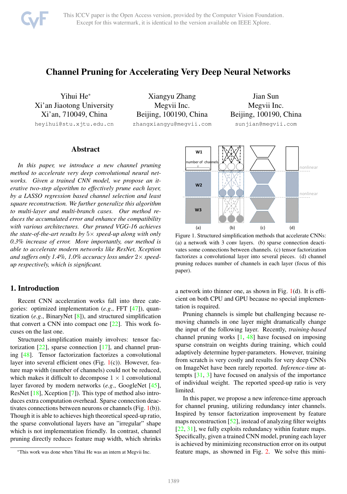
Channel Pruning for Accelerating Very Deep Neural Networks

Yihui HeXiangyu ZhangJian Sun

article2017ICCV2,806 citations

Proposes an effective channel pruning method combining LASSO-based channel selection with least-squares feature reconstruction to accelerate deep convolutional networks like ResNet and VGG up to fivefold with minimal accuracy loss.

Listen

Deep convolutional neural networks deliver high accuracy on image tasks but incur substantial inference costs on standard hardware. This creates pressure to accelerate them without major accuracy loss, especially for very deep models used in recognition, detection, and segmentation.

The article sets out to develop and test an inference-time channel pruning method that shrinks feature-map width layer by layer while keeping reconstruction error low. The method selects representative channels via LASSO regression and reconstructs outputs via least squares, then extends the procedure to entire models and multi-branch architectures such as residual blocks.

Experiments were run on VGG-16, ResNet-50, and Xception-50 using ImageNet, CIFAR-10, and PASCAL VOC 2007. Channel selection and reconstruction were applied sequentially, with sampling adjustments for shared feature maps in residual networks, followed by brief fine-tuning.

The pruned VGG-16 reached 5× speedup with only a 0.3 % rise in top-5 error and 4× speedup with a 1.0 % rise. ResNet-50 and Xception-50 achieved 2× speedup at 1.4 % and 1.0 % accuracy loss, respectively. The approach outperformed prior channel-pruning and tensor-factorization baselines on both accuracy and measured GPU runtime.

These results show that substantial redundancy exists across channels in trained networks and that removing it at inference time yields compact models that run efficiently on ordinary libraries and hardware. The gains translate directly into lower latency and energy use for deployed vision systems.

The authors recommend combining channel pruning with spatial and channel factorization for further compression and suggest extending the technique into the training phase to shorten training as well. Additional work on very deep modern architectures and larger-scale datasets would strengthen before widespread adoption.

The main limitations are that modern networks contain less redundancy by design, so accuracy drops are larger than for VGG-16, and that fine-tuning is required to reach the best reported numbers. Results rest on empirical tests across standard benchmarks and appear reliable within those conditions.

Cover for Channel Pruning for Accelerating Very Deep Neural Networks

Abstract

In this paper, we introduce a new channel pruning method to accelerate very deep convolutional neural this http URL a trained CNN model, we propose an iterative two-step algorithm to effectively prune each layer, by a LASSO regression based channel selection and least square reconstruction. We further generalize this algorithm to multi-layer and multi-branch cases. Our method reduces the accumulated error and enhance the compatibility with various architectures. Our pruned VGG-16 achieves the state-of-the-art results by 5x speed-up along with only 0.3% increase of error. More importantly, our method is able to accelerate modern networks like ResNet, Xception and suffers only 1.4%, 1.0% accuracy loss under 2x speed-up respectively, which is significant. Code has been made publicly available.

Table of Contents

  • 1 Introduction
  • 2 Related Work
  • 3 Approach
  • 3.1 Formulation
  • 3.2 Whole Model Pruning
  • 3.3 Pruning Multi-Branch Networks
  • 4 Experiment
  • 4.1 Experiments with VGG-16
  • 4.1.1 Single Layer Pruning
  • 4.1.2 Whole Model Pruning
  • 4.1.3 Comparisons of Absolute Performance
  • 4.1.4 Comparisons with Training from Scratch
  • 4.1.5 Acceleration for Detection
  • 4.2 Experiments with Residual Architecture Nets
  • 4.2.1 ResNet Pruning
  • 4.2.2 Xception Pruning
  • 4.2.3 Experiments on CIFAR-10
  • 5 Conclusion
  • References

Knowls

  1. Knowl 1 — LASSO-Based Formulation and Two-Step Optimization for Single-Layer Channel Pruning

    algorithm

    To prune the input channels of a convolutional layer from cc channels to a target count cc' (0cc0 \le c' \le c) while preserving network activations, channel pruning is formulated as minimizing the reconstruction error of the output feature maps. Let XRN×c×kh×kwX \in \mathbb{R}^{N \times c \times k_h \times k_w} represent NN input volume patches sampled from the input feature map, where kh×kwk_h \times k_w is the spatial kernel size. Let WRn×c×kh×kwW \in \mathbb{R}^{n \times c \times k_h \times k_w} denote the convolutional filter weights producing an output matrix YRN×nY \in \mathbb{R}^{N \times n} across nn output channels. Slicing along channel ii gives input slice XiRN×khkwX_i \in \mathbb{R}^{N \times k_h k_w} and filter slice WiRn×khkwW_i \in \mathbb{R}^{n \times k_h k_w}.

    The 0\ell_0 channel selection objective is relaxed to an 1\ell_1-regularized LASSO formulation with unit filter norm constraints:

    argminβ,W12NYi=1cβiXiWiF2+λβ1subject to β0c,  i,WiF=1\arg\min_{\beta, W} \frac{1}{2N} \left\| Y - \sum_{i=1}^c \beta_i X_i W_i^\top \right\|_F^2 + \lambda \|\beta\|_1 \quad \text{subject to } \|\beta\|_0 \le c', \; \forall i, \|W_i\|_F = 1

    where β=[β1,,βc]Rc\beta = [\beta_1, \dots, \beta_c]^\top \in \mathbb{R}^c is a channel selection coefficient vector, λ0\lambda \ge 0 is a sparsity penalty parameter, and F\|\cdot\|_F is the Frobenius norm. Setting βi=0\beta_i = 0 prunes the ii-th input channel and its associated filter parameters WiW_i.

    The optimization alternates between two subproblems: (1) solving for β\beta via LASSO regression while keeping WW fixed with Zi=XiWiRN×nZ_i = X_i W_i^\top \in \mathbb{R}^{N \times n}, and (2) solving for WW via linear least squares on the selected subset while keeping β\beta fixed. For computational efficiency, λ\lambda is gradually increased to solve the LASSO subproblem multiple times until β0c\|\beta\|_0 \le c', after which the least-squares reconstruction step is solved once.

    Input: Input patch matrix XRN×c×kh×kwX \in \mathbb{R}^{N \times c \times k_h \times k_w}, output feature map YRN×nY \in \mathbb{R}^{N \times n}, trained weights WRn×c×kh×kwW \in \mathbb{R}^{n \times c \times k_h \times k_w}, target channel count cc', penalty step Δλ>0\Delta \lambda > 0
    Output: Pruned and reconstructed filter weights WRn×c×kh×kwW^* \in \mathbb{R}^{n \times c' \times k_h \times k_w}
    Initialize λ0\lambda \leftarrow 0
    For each channel i{1,,c}i \in \{1, \dots, c\}:
        Xislice of X for channel i(N×khkw)X_i \leftarrow \text{slice of } X \text{ for channel } i \quad (N \times k_h k_w)
        Wislice of W for channel i(n×khkw)W_i \leftarrow \text{slice of } W \text{ for channel } i \quad (n \times k_h k_w)
        ZiXiWi(N×n)Z_i \leftarrow X_i W_i^\top \quad (N \times n)
    β[1,1,,1]\beta \leftarrow [1, 1, \dots, 1]^\top
    while β0>c\|\beta\|_0 > c' do:
        λλ+Δλ\lambda \leftarrow \lambda + \Delta \lambda
        βargminβ12NYi=1cβiZiF2+λβ1\beta \leftarrow \arg\min_{\beta} \frac{1}{2N} \|Y - \sum_{i=1}^c \beta_i Z_i\|_F^2 + \lambda \|\beta\|_1
    S{iβi0}S \leftarrow \{i \mid \beta_i \neq 0\} (indices of selected channels, Sc|S| \le c')
    X[βiXi]iS(N×Skhkw)X' \leftarrow [\beta_i X_i]_{i \in S} \quad (N \times |S| k_h k_w)
    WargminWYX(W)F2(n×Skhkw)W' \leftarrow \arg\min_{W'} \|Y - X' (W')^\top\|_F^2 \quad (n \times |S| k_h k_w)
    Reshape WW' into tensor WRn×S×kh×kwW^* \in \mathbb{R}^{n \times |S| \times k_h \times k_w}
    return WW^*
  2. Knowl 2 — Layer-by-Layer Sequential Whole-Model Pruning with Accumulated Error Compensation

    model/method

    When pruning multi-layer networks sequentially from shallow to deep layers, local errors in early layers can compound and degrade downstream feature representations. To eliminate error accumulation, the reconstruction target for each layer is tied to the original unpruned network rather than the preceding pruned layer's output.

    For each sequential layer, let XiRN×khkwX_i \in \mathbb{R}^{N \times k_h k_w} denote the input feature volumes generated by passing training samples through the preceding already-pruned layers. Let YRN×nY' \in \mathbb{R}^{N \times n} denote the output feature map volumes sampled from the corresponding layer in the original, unpruned baseline model. The sequential pruning optimization is formulated as:

    argminβ,W12NYi=1cβiXiWiF2+λβ1subject to β0c,  i,WiF=1\arg\min_{\beta, W} \frac{1}{2N} \left\| Y' - \sum_{i=1}^c \beta_i X_i W_i^\top \right\|_F^2 + \lambda \|\beta\|_1 \quad \text{subject to } \|\beta\|_0 \le c', \; \forall i, \|W_i\|_F = 1

    Because the linear least squares reconstruction step targets YY', the updated weights at the current layer actively compensate for the accumulated spatial and channel discrepancies introduced by earlier layers. Pruning allocations are structured to prune shallow layers (e.g., conv1_x to conv3_x) more aggressively than deeper layers (conv4_x), while leaving computationally inexpensive and sensitive final feature extraction layers (e.g., conv5_x, accounting for only 9% of total FLOPs in VGG-16) unpruned.

  3. Knowl 3 — Channel Pruning Adaptations for Multi-Branch Residual Architectures

    model/method

    Standard sequential channel pruning cannot be directly applied to multi-branch residual blocks (such as in ResNet and Xception) because identity shortcuts share representations with residual branches and contain no parameters to absorb error. Two modifications enable pruning residual blocks:

    1. Input Feature Map Sampling for First Residual Layer: The input feature map with c0c_0 channels at the entrance of a residual block is fed simultaneously into the residual branch (starting with a 1×11 \times 1 convolution) and the identity shortcut. Removing channels globally from c0c_0 would alter the shortcut output. To circumvent this, a channel sampling operation is placed immediately before the first 1×11 \times 1 convolution of the residual branch. The LASSO selection identifies a representative subset of c0c_0' channels from c0c_0, and only these sampled channels are fed into the first convolutional layer, preserving standard regular convolution tensor shapes without modifying the shared shortcut branch.

    2. Shortcut Error Compensation for Last Residual Layer: The output of a residual block is Y=Y1+Y2Y = Y_1 + Y_2, where Y1Y_1 is the shortcut feature map and Y2Y_2 is the residual branch feature map. When previous blocks are pruned, the shortcut feature map shifts to Y1Y_1', and because the identity shortcut has no learnable weights, the shortcut error Y1Y1Y_1 - Y_1' cannot be corrected directly. To compensate, the reconstruction objective for the last layer of the residual branch is modified from approximating Y2Y_2 to reconstructing:

    Ytarget=Y1Y1+Y2Y_{\text{target}} = Y_1 - Y_1' + Y_2

    where Y1Y_1 and Y2Y_2 are the unpruned reference feature maps from the shortcut and residual branches, and Y1Y_1' is the feature map produced by the shortcut under the current pruned state. The least squares solver adjusts the final residual layer's weights to fit YtargetY_{\text{target}}, canceling the accumulated shortcut discrepancy.

  4. Knowl 4 — Three-Cardinality CNN Acceleration Combining Spatial Factorization, Channel Factorization, and Channel Pruning

    model/method

    Convolutional redundancy can be exploited across three orthogonal cardinalities: spatial decomposition, cross-channel decomposition, and channel pruning. The combined 3C acceleration scheme applies all three operations sequentially layer-by-layer:

    1. Spatial Factorization: Decomposing a 2D spatial convolution kernel (e.g., kh×kw=3×3k_h \times k_w = 3 \times 3) into two low-rank 1D spatial filters (1×31 \times 3 and 3×13 \times 1).
    2. Channel Factorization: Decomposing the cross-channel feature projection into a linear combination via a 1×11 \times 1 convolutional layer.
    3. Channel Pruning: Applying LASSO channel selection and linear least-squares output reconstruction to reduce the total number of input and intermediate channels.

    Because the resulting 3C architecture contains roughly three times as many layers as the original baseline model, the pruned and factorized network is fine-tuned for 20 epochs using stochastic gradient descent. Combining all three cardinalities outperforms applying any single acceleration technique in isolation at high acceleration ratios.

  5. Knowl 5 — Experimental Calibration and Fine-Tuning Setup for Channel Pruning

    experimental setup

    The channel pruning pipeline and evaluation are configured as follows across ImageNet, CIFAR-10, and PASCAL VOC 2007:

    • Batch Normalization Absorption: Prior to pruning, Batch Normalization parameters are absorbed directly into the convolutional filter weights and biases so that each convolutional layer is followed immediately by a ReLU activation. For Xception architectures, Batch Normalization layers are retained during pruning to maintain optimization stability.
    • Calibration Dataset for Regression: Linear regression and LASSO subproblems are constructed by extracting N=50,000N = 50,000 volume samples (10 random spatial volume patches per image from 5,000 sampled ImageNet training images).
    • Fine-Tuning Hyperparameters: Pruned models on ImageNet are fine-tuned for 10 epochs (20 epochs for 3C factorized models) using a mini-batch size of 128, a constant learning rate of 1×1051 \times 10^{-5}, and training data augmentation consisting of random cropping to 224×224224 \times 224 pixels and random horizontal flipping.
    • Evaluation Protocols: ImageNet classification is measured using single-crop (224×224224 \times 224 center crop, shorter side resized to 256) top-5 accuracy. Baseline unpruned single-view top-5 accuracies are 89.9% for VGG-16, 92.2% for ResNet-50, and 92.8% for Xception-50.
  6. Knowl 6 — Whole-Model VGG-16 Acceleration and Error Comparison Across Pruning Methods

    data/table

    Whole-model pruning evaluation on VGG-16 on ImageNet (baseline top-5 single-view accuracy 89.9%) at theoretical FLOP speedup ratios of 2×2\times, 4×4\times, and 5×5\times. Shallow layers (conv1_x to conv3_x) and deep layers (conv4_x) use a remaining channel ratio of 1:1.51 : 1.5, while conv5_x layers remain unpruned.

    Solution 2×2\times 4×4\times 5×5\times
    Jaderberg et al. (spatial factorization) - 9.7% 29.7%
    Asymmetric Factorization 0.28% 3.84% -
    Filter pruning (Li et al., fine-tuned) 0.8% 8.6% 14.6%
    Ours (without fine-tuning) 2.7% 7.9% 22.0%
    Ours (fine-tuned 10 epochs) 0.0% 1.0% 1.7%

    Values represent the increase in top-5 error percentage relative to the baseline (lower is better). After fine-tuning, the proposed channel pruning method achieves 2×2\times speedup with 0.0% error increase and 4×4\times speedup with 1.0% error increase, outperforming weight-magnitude filter pruning (Li et al.) by 7.6 percentage points at 4×4\times speedup.

  7. Knowl 7 — Comparison of Combined 3C Acceleration on VGG-16

    data/table

    Performance of the three-cardinality combination (spatial factorization, channel factorization, and channel pruning, denoted 3C) compared against asymmetric 3D tensor factorization on VGG-16 on ImageNet under 4×4\times and 5×5\times theoretical speedup ratios.

    Solution 4×4\times 5×5\times
    Asymmetric 3D (without fine-tuning) 0.9% 2.0%
    Asymmetric 3D (fine-tuned) 0.3% 1.0%
    Our 3C (without fine-tuning) 0.7% 1.3%
    Our 3C (fine-tuned 20 epochs) 0.0% 0.3%

    Values denote the increase in top-5 error percentage on ImageNet (baseline 89.9% top-5 accuracy, lower is better). Combining channel pruning with spatial and channel tensor factorization eliminates accuracy degradation at 4×4\times acceleration (0.0%0.0\% error increase) and achieves 5×5\times acceleration with only a 0.3%0.3\% error increase.

  8. Knowl 8 — GPU Latency and Forward Inference Speedup of Channel Pruning Versus Tensor Factorization

    data/table

    Comparison of theoretical acceleration versus actual inference forward-pass execution time on a GPU (NVIDIA GeForce GTX TITAN X, CUDA 8, cuDNN 5, mini-batch size 32, averaged over 50 runs) on VGG-16 at a 4×4\times theoretical FLOP speedup setting.

    Model / Solution Increased Top-5 Error (%) GPU Forward Time (ms) / Speedup
    VGG-16 Baseline 0.0% 8.144 ms (1.00×1.00\times)
    Jaderberg et al. (4×4\times) 9.7% 8.051 ms (1.01×1.01\times)
    Asymmetric Factorization (4×4\times) 3.8% 5.244 ms (1.55×1.55\times)
    Asym. 3D (4×4\times) 0.9% 8.503 ms (0.96×0.96\times)
    Asym. 3D fine-tuned (4×4\times) 0.3% 8.503 ms (0.96×0.96\times)
    Ours fine-tuned (4×4\times) 1.0% 3.264 ms (2.50×2.50\times)

    Tensor factorization decomposes single convolutions into multiple smaller sequential convolutions, introducing computational kernel launch and memory bandwidth overhead that reduces or inverts GPU acceleration (0.96×0.96\times to 1.55×1.55\times actual speedup). Channel pruning shrinks feature tensor widths while maintaining standard dense convolutional shapes, achieving an actual GPU speedup of 2.50×2.50\times (reducing latency from 8.144 ms to 3.264 ms per batch).

  9. Knowl 9 — Accuracy Comparison of Channel Pruning Versus Training From Scratch

    data/table

    Comparison of a 4×4\times channel-pruned VGG-16 against identical-complexity compact architectures trained from scratch for 120 epochs on ImageNet (baseline unpruned VGG-16 top-5 error is 10.1%, corresponding to 89.9% top-5 accuracy).

    Model Configuration Top-5 Error (%) Increased Error (%)
    Unpruned Baseline 10.1% 0.0%
    From scratch (same non-uniform channel counts) 11.9% 1.8%
    From scratch (uniformed: channels halved in each layer) 12.5% 2.4%
    Ours (without fine-tuning) 18.0% 7.9%
    Ours (fine-tuned 10 epochs) 11.1% 1.0%

    The fine-tuned channel-pruned model achieves 11.1% top-5 error (+1.0% over baseline), outperforming the exact same non-uniform architecture trained from scratch by 0.8% and the uniformly thinned model trained from scratch by 1.4%. This indicates that overparameterized optimization during initial training discovers representations that can be compressed at inference time, which training thin networks from scratch fails to reach.

  10. Knowl 10 — Channel Pruning Acceleration on ResNet-50 and Xception-50 on ImageNet

    data/table

    Evaluation of 2×2\times theoretical FLOP acceleration on residual networks (ResNet-50, baseline top-5 accuracy 92.2%) and depthwise separable networks (Xception-50, baseline top-5 accuracy 92.8%, 4450 MFLOPs) on ImageNet. In ResNet-50, sensitive residual blocks (res5 and spatial transition blocks) retain 70% of channels, while remaining blocks retain 30% overall (with internal ratios for branch2a, branch2b, and branch2c set to 2:4:32:4:3, corresponding to 40%, 80%, and 60% channel retention).

    Network Acceleration Solution Increased Top-5 Error (%)
    ResNet-50 (2×2\times) Ours (standard pruning without multi-branch adaptation) 8.0%
    ResNet-50 (2×2\times) Ours (multi-branch enhanced, without fine-tuning) 4.0%
    ResNet-50 (2×2\times) Ours (multi-branch enhanced, fine-tuned 10 epochs) 1.4%
    Xception-50 (2×2\times) Filter pruning (Li et al., without fine-tuning) 92.8%
    Xception-50 (2×2\times) Filter pruning (Li et al., fine-tuned 20 epochs) 4.3%
    Xception-50 (2×2\times) Ours (without fine-tuning) 2.9%
    Xception-50 (2×2\times) Ours (fine-tuned 10 epochs) 1.0%

    The multi-branch adaptation halves the un-fine-tuned error increase from 8.0% to 4.0% on ResNet-50. On Xception-50, which uses 1×11 \times 1 convolutions and depthwise separable convolutions that resist tensor factorization, channel pruning maintains accuracy within 1.0% error increase after fine-tuning.

  11. Knowl 11 — Transfer Learning Performance on Faster R-CNN Detection and CIFAR-10 Classification

    empirical result

    Channel-pruned backbones retain strong generalization when transferred to downstream tasks and smaller datasets:

    • Faster R-CNN Object Detection on PASCAL VOC 2007: Using ImageNet-pretrained 2×2\times and 4×4\times pruned VGG-16 models as backbones for Faster R-CNN (baseline mAP is 68.7% with 220 ms/image latency, where convolutional layers take 64% of runtime):

      • A 2×2\times accelerated backbone yields 68.3% mAP (a drop of 0.4% mAP).
      • A 4×4\times accelerated backbone yields 66.9% mAP (a drop of 1.8% mAP) while reducing total detector inference latency from 220 ms to 94 ms per image.
    • ResNet-56 Acceleration on CIFAR-10: On CIFAR-10 classification (reproduced baseline top-1 accuracy 92.8% for ResNet-56) under 2×2\times FLOP speedup (keeping the final 8×88 \times 8 stage unpruned):

      • Filter weight pruning (Li et al., fine-tuned) has a 1.3% accuracy loss (91.5% accuracy).
      • An equivalent compact ResNet-56 trained from scratch has a 1.9% accuracy loss (90.9% accuracy).
      • Ours without fine-tuning has a 2.0% accuracy loss (90.8% accuracy).
      • Ours after fine-tuning achieves a 1.0% accuracy loss (91.8% accuracy), outperforming both filter weight pruning and training from scratch.

Coverage note — All core contributions, mathematical formulations, algorithms, multi-branch residual extensions, three-cardinality combinations, and benchmark results on VGG-16, ResNet-50, Xception-50, CIFAR-10, and PASCAL VOC 2007 are covered; only secondary exploratory variations such as filter-wise pruning on residual branches (which produced irregular non-standard layers and showed no post-fine-tuning benefit) were omitted.

References

  1. 1.J. M. Alvarez and M. Salzmann. Learning the number of neurons in deep networks. In Advances in Neural Information Processing Systems, pages 2262–2270, 2016. 1, 2, 3, 6
  2. 2.S. Anwar, K. Hwang, and W. Sung. Structured pruning of deep convolutional neural networks. arXiv preprint arXiv:1512.08571, 2015. 2
  3. 3.S. Anwar and W. Sung. Compact deep convolutional neural networks with coarse pruning. arXiv preprint arXiv:1610.09639, 2016. 1, 2
  4. 4.H. Bagherinezhad, M. Rastegari, and A. Farhadi. Lcnn: Lookup-based convolutional neural network. arXiv preprint arXiv:1611.06473, 2016. 2
  5. 5.L. Breiman. Better subset regression using the nonnegative garrote. Technometrics, 37(4):373–384, 1995. 3
  6. 6.S. Chetlur, C. Woolley, P. Vandermersch, J. Cohen, J. Tran, B. Catanzaro, and E. Shelhamer. cudnn: Efficient primitives for deep learning. CoRR, abs/1410.0759, 2014. 6
  7. 7.F. Chollet. Xception: Deep learning with depthwise separable convolutions. arXiv preprint arXiv:1610.02357, 2016. 1, 2, 3, 4, 6, 7
  8. 8.M. Courbariaux and Y. Bengio. Binarynet: Training deep neural networks with weights and activations constrained to+ 1 or-1. arXiv preprint arXiv:1602.02830, 2016. 1, 2
  9. 9.J. Deng, W. Dong, R. Socher, L.-J. Li, K. Li, and L. Fei-Fei. Imagenet: A large-scale hierarchical image database. In Computer Vision and Pattern Recognition, 2009. CVPR 2009. IEEE Conference on, pages 248–255. IEEE, 2009. 4
  10. 10.E. L. Denton, W. Zaremba, J. Bruna, Y. LeCun, and R. Fergus. Exploiting linear structure within convolutional networks for efficient evaluation. In Advances in Neural Information Processing Systems, pages 1269–1277, 2014. 2
  11. 11.M. Everingham, L. Van Gool, C. K. I. Williams, J. Winn, and A. Zisserman. The PASCAL Visual Object Classes Challenge 2007 (VOC2007) Results. http://www.pascalnetwork.org/challenges/VOC/voc2007/workshop/index.html. 4, 6
  12. 12.R. Girshick. Fast r-cnn. In Proceedings of the IEEE International Conference on Computer Vision, pages 1440–1448, 2015. 2
  13. 13.Y. Gong, L. Liu, M. Yang, and L. Bourdev. Compressing deep convolutional networks using vector quantization. arXiv preprint arXiv:1412.6115, 2014. 2
  14. 14.Y. Guo, A. Yao, and Y. Chen. Dynamic network surgery for efficient dnns. In Advances In Neural Information Processing Systems, pages 1379–1387, 2016. 2
  15. 15.S. Han, X. Liu, H. Mao, J. Pu, A. Pedram, M. A. Horowitz, and W. J. Dally. Eie: efficient inference engine on compressed deep neural network. In Proceedings of the 43rd International Symposium on Computer Architecture, pages 243–254. IEEE Press, 2016. 2
  16. 16.S. Han, H. Mao, and W. J. Dally. Deep compression: Compressing deep neural network with pruning, trained quantization and huffman coding. CoRR, abs/1510.00149, 2, 2015. 2
  17. 17.S. Han, J. Pool, J. Tran, and W. Dally. Learning both weights and connections for efficient neural network. In Advances in Neural Information Processing Systems, pages 1135–1143, 2015. 1, 2, 3
  18. 18.K. He, X. Zhang, S. Ren, and J. Sun. Deep residual learning for image recognition. arXiv preprint arXiv:1512.03385, 2015. 1, 2, 3, 4, 6, 8
  19. 19.H. Hu, R. Peng, Y.-W. Tai, and C.-K. Tang. Network trimming: A data-driven neuron pruning approach towards efficient deep architectures. arXiv preprint arXiv:1607.03250, 2016. 2
  20. 20.J. Huang, V. Rathod, C. Sun, M. Zhu, A. Korattikara, A. Fathi, I. Fischer, Z. Wojna, Y. Song, S. Guadarrama, et al. Speed/accuracy trade-offs for modern convolutional object detectors. arXiv preprint arXiv:1611.10012, 2016. 6
  21. 21.S. Ioffe and C. Szegedy. Batch normalization: Accelerating deep network training by reducing internal covariate shift. arXiv preprint arXiv:1502.03167, 2015. 4
  22. 22.M. Jaderberg, A. Vedaldi, and A. Zisserman. Speeding up convolutional neural networks with low rank expansions. arXiv preprint arXiv:1405.3866, 2014. 1, 2, 5, 6, 7
  23. 23.Y. Jia, E. Shelhamer, J. Donahue, S. Karayev, J. Long, R. Girshick, S. Guadarrama, and T. Darrell. Caffe: Convolutional architecture for fast feature embedding. arXiv preprint arXiv:1408.5093, 2014. 4, 6
  24. 24.Y.-D. Kim, E. Park, S. Yoo, T. Choi, L. Yang, and D. Shin. Compression of deep convolutional neural networks for fast and low power mobile applications. arXiv preprint arXiv:1511.06530, 2015. 2
  25. 25.A. Krizhevsky and G. Hinton. Learning multiple layers of features from tiny images. 2009. 4, 8
  26. 26.A. Krizhevsky, I. Sutskever, and G. E. Hinton. Imagenet classification with deep convolutional neural networks. In Advances in neural information processing systems, pages 1097–1105, 2012. 2, 3
  27. 27.A. Lavin. Fast algorithms for convolutional neural networks. arXiv preprint arXiv:1509.09308, 2015. 2
  28. 28.V. Lebedev, Y. Ganin, M. Rakhuba, I. Oseledets, and V. Lempitsky. Speeding-up convolutional neural networks using fine-tuned cp-decomposition. arXiv preprint arXiv:1412.6553, 2014. 2
  29. 29.V. Lebedev and V. Lempitsky. Fast convnets using groupwise brain damage. arXiv preprint arXiv:1506.02515, 2015. 2
  30. 30.Y. LeCun, L. Bottou, Y. Bengio, and P. Haffner. Gradient-based learning applied to document recognition. Proceedings of the IEEE, 86(11):2278–2324, 1998. 2, 3
  31. 31.H. Li, A. Kadav, I. Durdanovic, H. Samet, and H. P. Graf. Pruning filters for efficient convnets. arXiv preprint arXiv:1608.08710, 2016. 1, 2, 4, 5, 6, 7, 8
  32. 32.B. Liu, M. Wang, H. Foroosh, M. Tappen, and M. Pensky. Sparse convolutional neural networks. In Proceedings of the IEEE Conference on Computer Vision and Pattern Recognition, pages 806–814, 2015. 2
  33. 33.W. Liu, D. Anguelov, D. Erhan, C. Szegedy, S. E. Reed, C. Fu, and A. C. Berg. SSD: single shot multibox detector. CoRR, abs/1512.02325, 2015. 6
  34. 34.Z. Mariet and S. Sra. Diversity networks. arXiv preprint arXiv:1511.05077, 2015. 2
  35. 35.M. Mathieu, M. Henaff, and Y. LeCun. Fast training of convolutional networks through ffts. arXiv preprint arXiv:1312.5851, 2013. 2
  36. 36.V. Nair and G. E. Hinton. Rectified linear units improve restricted boltzmann machines. In Proceedings of the 27th international conference on machine learning (ICML-10), pages 807–814, 2010. 4
  37. 37.J. Nickolls, I. Buck, M. Garland, and K. Skadron. Scalable parallel programming with CUDA. ACM Queue, 6(2):40–53, 2008. 6
  38. 38.F. Pedregosa, G. Varoquaux, A. Gramfort, V. Michel, B. Thirion, O. Grisel, M. Blondel, P. Prettenhofer, R. Weiss, V. Dubourg, J. Vanderplas, A. Passos, D. Cournapeau, M. Brucher, M. Perrot, and E. Duchesnay. Scikit-learn: Machine learning in Python. Journal of Machine Learning Research, 12:2825–2830, 2011. 4
  39. 39.A. Polyak and L. Wolf. Channel-level acceleration of deep face representations. IEEE Access, 3:2163–2175, 2015. 2
  40. 40.M. Rastegari, V. Ordonez, J. Redmon, and A. Farhadi. Xnornet: Imagenet classification using binary convolutional neural networks. In European Conference on Computer Vision, pages 525–542. Springer, 2016. 2
  41. 41.J. Redmon, S. K. Divvala, R. B. Girshick, and A. Farhadi. You only look once: Unified, real-time object detection. CoRR, abs/1506.02640, 2015. 6
  42. 42.S. Ren, K. He, R. B. Girshick, and J. Sun. Faster R-CNN: towards real-time object detection with region proposal networks. CoRR, abs/1506.01497, 2015. 6
  43. 43.K. Simonyan and A. Zisserman. Very deep convolutional networks for large-scale image recognition. arXiv preprint arXiv:1409.1556, 2014. 3, 4, 5, 6
  44. 44.S. Srinivas and R. V. Babu. Data-free parameter pruning for deep neural networks. arXiv preprint arXiv:1507.06149, 2015. 2
  45. 45.C. Szegedy, W. Liu, Y. Jia, P. Sermanet, S. Reed, D. Anguelov, D. Erhan, V. Vanhoucke, and A. Rabinovich. Going deeper with convolutions. In Proceedings of the IEEE Conference on Computer Vision and Pattern Recognition, pages 1–9, 2015. 1, 3, 6
  46. 46.R. Tibshirani. Regression shrinkage and selection via the lasso. Journal of the Royal Statistical Society. Series B (Methodological), pages 267–288, 1996. 3
  47. 47.N. Vasilache, J. Johnson, M. Mathieu, S. Chintala, S. Piantino, and Y. LeCun. Fast convolutional nets with fbfft: A gpu performance evaluation. arXiv preprint arXiv:1412.7580, 2014. 1, 2
  48. 48.W. Wen, C. Wu, Y. Wang, Y. Chen, and H. Li. Learning structured sparsity in deep neural networks. In Advances In Neural Information Processing Systems, pages 2074–2082, 2016. 1, 2, 3
  49. 49.S. Xie, R. Girshick, P. Dollár, Z. Tu, and K. He. Aggregated residual transformations for deep neural networks. arXiv preprint arXiv:1611.05431, 2016. 7
  50. 50.J. Xue, J. Li, and Y. Gong. Restructuring of deep neural network acoustic models with singular value decomposition. In INTERSPEECH, pages 2365–2369, 2013. 2
  51. 51.T.-J. Yang, Y.-H. Chen, and V. Sze. Designing energyefficient convolutional neural networks using energy-aware pruning. arXiv preprint arXiv:1611.05128, 2016. 2
  52. 52.X. Zhang, J. Zou, K. He, and J. Sun. Accelerating very deep convolutional networks for classification and detection. IEEE transactions on pattern analysis and machine intelligence, 38(10):1943–1955, 2016. 1, 2, 3, 5, 6, 7

Citation

MLA
He, Y., et al. “Channel Pruning for Accelerating Very Deep Neural Networks”. arXiv, 2017, http://arxiv.org/abs/1707.06168v2.
APA
He, Y., Zhang, X., & Sun, J. (2017). Channel Pruning for Accelerating Very Deep Neural Networks. arXiv. http://arxiv.org/abs/1707.06168v2
Chicago
He, Y., X. Zhang, and J. Sun. 2017. “Channel Pruning for Accelerating Very Deep Neural Networks”. arXiv. http://arxiv.org/abs/1707.06168v2.
Harvard
He, Y., Zhang, X. and Sun, J. (2017) “Channel Pruning for Accelerating Very Deep Neural Networks”, arXiv [Preprint]. Available at: http://arxiv.org/abs/1707.06168v2.
Vancouver
1. He Y, Zhang X, Sun J (2017) Channel Pruning for Accelerating Very Deep Neural Networks. arXiv

BibTeX

@article{he2017channel,
  title = {Channel Pruning for Accelerating Very Deep Neural Networks},
  author = {He, Yihui and Zhang, Xiangyu and Sun, Jian},
  year = {2017},
  journal = {arXiv},
  url = {http://arxiv.org/abs/1707.06168v2},
  eprint = {1707.06168}
}
Metadata:arXiv

Source Code

This paper has an official code repository available. Click below to access the source code.

View Repository

Access the Paper

This paper is available from its original source. Click below to access the PDF.

Open PDF

License: IEEE