Pruning Convolutional Neural Networks for Resource Efficient Inference

Pavlo MolchanovStephen TyreeTero KarrasTimo AilaJan Kautz

article2016ICLR2,320 citations

Introduces a Taylor expansion-based pruning criterion that uses first-order gradient information to efficiently remove redundant convolutional filters, achieving up to a tenfold reduction in model size with minimal accuracy loss across transfer learning benchmarks.

Listen

Modern computer vision models achieve outstanding accuracy across image and video tasks, particularly when large pretrained models are adapted to specialized domains via transfer learning. However, running these deep convolutional networks requires significant processing time, memory, and electrical power. This computational burden creates severe bottlenecks when deploying models on resource-constrained embedded systems and mobile edge devices.

The article establishes and evaluates a structured method to compress convolutional neural networks by pruning entire feature maps to enable faster, low-power inference while maintaining model accuracy. The authors set out to determine an efficient pruning criterion that accurately approximates the importance of each feature map without incurring the heavy computational overhead of existing techniques.

To achieve this, the article introduces an iterative framework that alternates between removing the least important feature map and fine-tuning the remaining parameters using standard backpropagation. Parameter importance is estimated using a first-order Taylor expansion criterion, which directly approximates the absolute change in the model's loss function when a feature map is removed. The authors evaluated this approach against several benchmark criteria—such as weight magnitude, feature activation statistics, mutual information, and second-order methods like Optimal Brain Damage—across standard vision architectures (AlexNet, VGG-16, and recurrent 3D networks) and datasets (Birds-200, Oxford Flowers-102, and ImageNet) on multiple central processing unit (CPU) and graphics processing unit (GPU) platforms.

The findings show that the proposed first-order Taylor criterion achieves the highest rank correlation with the theoretical benchmark (the exhaustive oracle) while requiring only standard first-order gradients. Pruning entire feature maps directly translates to substantial, practical run-time speedups on standard hardware without requiring specialized sparse-matrix processors. For example, on a recurrent 3D gesture recognition network, the method reduced floating-point operations by over 12-fold, yielding a 5.2x wall-clock speedup on an embedded GPU with only a 2.5% loss in accuracy. On fine-grained image tasks, the models maintained strong classification accuracy across substantial pruning ratios, outperforming traditional weight-regularization techniques. Additionally, the analysis established that applying layer-wise normalization and computation-aware regularization is essential for maintaining a balanced pruning distribution across network layers.

These results demonstrate that organizations can significantly lower edge deployment costs, memory footprints, and latency risks for computer vision models without sacrificing competitive predictive accuracy. Unlike unstructured weight pruning—which often requires specialized hardware to realize actual speed gains—channel-level pruning produces immediate operational acceleration on commodity hardware. Furthermore, by relying strictly on first-order gradient statistics readily produced during regular backpropagation, the pruning process itself avoids the prohibitive computational and memory costs associated with second-order derivative calculations.

Organizations seeking to deploy deep vision models to resource-constrained environments should adopt this greedy, criterion-based structured pruning workflow alongside floating-point regularization. Teams should plan for incremental fine-tuning between pruning steps and consider a short period of post-pruning optimization to recover minor accuracy losses. In terms of limitations, actual hardware speedup varies depending on convolution implementations, batch sizes, memory transfer bandwidth, and specific GPU architectures. While the findings provide high confidence for standard vision architectures adapted via transfer learning, teams should validate performance on target edge hardware through pilot testing before large-scale deployment.

NVIDIA backpropagation algorithm classification methods classifiers Pruning Feature Feature Maps

arXiv: 1611.06440

Paper: Learning both Weights and Connections for Efficient Neural Networks, Song Han et al. (2015). Reading this foundational study on magnitude pruning for sparse neural networks provides essential context for understanding the source paper's parameter-reduction techniques.
Paper: Pruning Filters for Efficient ConvNets, Hao Li et al. (2016). This earlier work on pruning entire convolutional filters provides the core methodology and motivation for the layer-wise sensitivity analysis and kernel-removal strategies expanded upon in the source paper.

Paper: Rethinking the Value of Network Pruning, Zhuang Liu et al. (2019). This paper challenges conventional pruning assumptions by demonstrating that training pruned architectures from scratch often matches or exceeds fine-tuning, directly extending the methodology introduced in the source.
Paper: Comparing Rewinding and Fine-tuning in Neural Network Pruning, Alex Renda et al. (2020). Building directly on the pruning framework established in the source, this work evaluates advanced retraining strategies like weight and learning rate rewinding to optimize post-pruning accuracy recovery.
Paper: The Lottery Ticket Hypothesis: Finding Sparse, Trainable Neural Networks., Jonathan Frankle et al. (2019). This study continues the investigation of pruned networks by uncovering trainable sparse subnetworks or winning tickets, extending the concepts of parameter efficiency explored in the source.

Cover for Pruning Convolutional Neural Networks for Resource Efficient Inference

Abstract

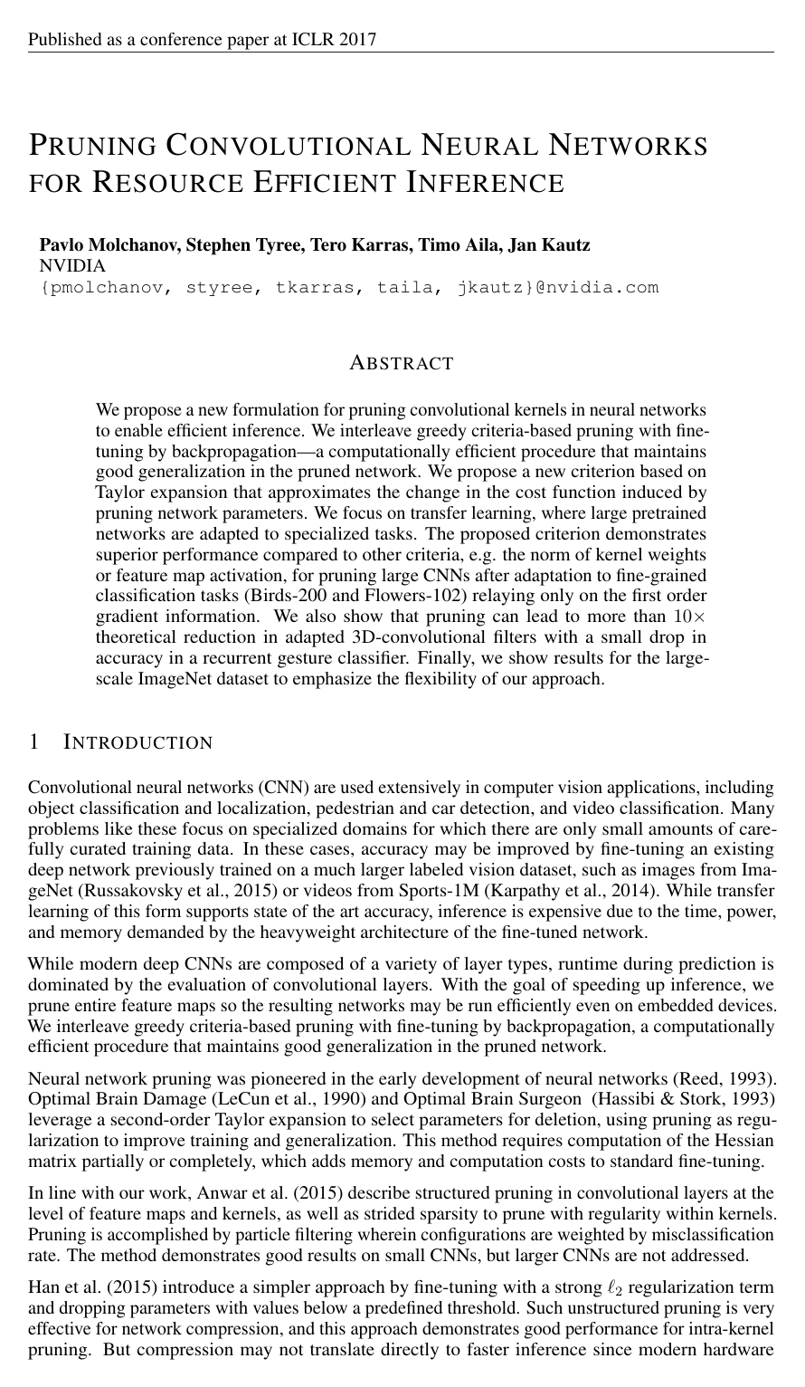
We propose a new formulation for pruning convolutional kernels in neural networks to enable efficient inference. We interleave greedy criteria-based pruning with fine-tuning by backpropagation - a computationally efficient procedure that maintains good generalization in the pruned network. We propose a new criterion based on Taylor expansion that approximates the change in the cost function induced by pruning network parameters. We focus on transfer learning, where large pretrained networks are adapted to specialized tasks. The proposed criterion demonstrates superior performance compared to other criteria, e.g. the norm of kernel weights or feature map activation, for pruning large CNNs after adaptation to fine-grained classification tasks (Birds-200 and Flowers-102) relaying only on the first order gradient information. We also show that pruning can lead to more than 10x theoretical (5x practical) reduction in adapted 3D-convolutional filters with a small drop in accuracy in a recurrent gesture classifier. Finally, we show results for the large-scale ImageNet dataset to emphasize the flexibility of our approach.

Topics

backpropagation algorithm classification methods classifiers convolutional neural networks inference out-of-distribution generalization transfer learning network architecture probabilistic inference

Keywords

Pruning Feature Feature Maps Convolutional Networks Neural Network Neural Networks Taylor Convolutional Neural Networks

1 Introduction
2 Method
2.1 Oracle pruning
2.2 Criteria for pruning
2.3 Normalization
2.4 FLOPs regularized pruning
3 Results
3.1 Characterizing the oracle ranking
3.2 Evaluating proposed criteria versus the oracle
3.3 Pruning fine-tuned ImageNet networks
3.4 Pruning a recurrent 3D-CNN network for hand gesture recognition
3.5 Pruning networks for ImageNet
3.6 Speed up measurements
4 Conclusions
References
A Appendix
A.1 FLOPs computation
A.2 Normalization across layers
A.3 Oracle computation for VGG-16 on Birds-200
A.4 Comparison with weight regularization
A.5 Combination of criteria
A.6 Optimal Brain Damage implementation
A.7 Correlation of Taylor criterion with gradient and activation

Knowls

Knowl 1 — First-Order Taylor Expansion Pruning Criterion for Feature Maps
model/method
To evaluate the importance (saliency) of individual convolutional feature maps without exhaustive evaluation, the change in the training loss function $\mathcal{C}(\mathcal{D}|W)$ caused by removing a feature map $h_i$ (setting $h_i = 0$ ) is approximated using a first-order Taylor expansion around $h_i = 0$ :

$\mathcal{C}(\mathcal{D}, h_i = 0) = \mathcal{C}(\mathcal{D}, h_i) - \frac{\partial \mathcal{C}}{\partial h_i} h_i + R_1(h_i = 0)$

Neglecting the remainder term $R_1(h_i = 0)$ , the absolute change in cost $|\Delta \mathcal{C}(h_i)| = |\mathcal{C}(\mathcal{D}, h_i = 0) - \mathcal{C}(\mathcal{D}, h_i)|$ yields the scalar parameter saliency criterion:

$\Theta_{TE}(h_i) = \left| \frac{\partial \mathcal{C}}{\partial h_i} h_i \right|$

For a convolutional layer outputting a feature map $z_l^{(k)} \in \mathbb{R}^{H_l \times W_l}$ with spatial height $H_l$ , width $W_l$ , and $M = H_l \times W_l$ elements, the Taylor expansion criterion is computed by averaging across the spatial coordinates:

$\Theta_{TE}(z_l^{(k)}) = \left| \frac{1}{M} \sum_{m=1}^M \frac{\partial \mathcal{C}}{\partial z_{l,m}^{(k)}} z_{l,m}^{(k)} \right|$

where $z_{l,m}^{(k)}$ is the activation of the $k$ -th feature map in layer $l$ at spatial index $m$ . For a minibatch of size $T > 1$ , the value is computed for each example independently and averaged across the minibatch. This criterion requires no second-order Hessian computation and can be evaluated directly from the activation values and intermediate backpropagation gradients.
Knowl 2 — Iterative Greedy Feature Map Pruning with Interleaved Fine-Tuning
algorithm
The greedy structured pruning framework removes convolutional feature maps one at a time, interleaved with backpropagation updates to maintain network stability and account for parameter interdependencies.
Input: Pretrained model with initial weights $W$ , training dataset $\mathcal{D}$ , target computational budget $B$ (e.g., target FLOPs or parameter count), number of fine-tuning SGD steps per pruning step $S$ , learning rate $\eta$
Output: Pruned network with weights $W^*$
Fine-tune $W$ on dataset $\mathcal{D}$ until validation loss converges
while Current FLOPs or active feature map count > $B$ do
    Evaluate layer-normalized Taylor saliency $\hat{\Theta}(z_l^{(k)})$ for every active feature map $k$ across all convolutional layers $l$
    Identify the least important feature map: $(l^*, k^*) = \arg\min_{l, k} \hat{\Theta}(z_l^{(k)})$
    Remove feature map $z_{l^*}^{(k^*)}$ and all incoming/outgoing kernel weights connected to it
    for step = 1 to $S$ do
        Sample minibatch from $\mathcal{D}$
        Perform forward and backward propagation
        Update remaining weights with SGD using learning rate $\eta$
    end for
end while
Optionally perform final fine-tuning of remaining weights until full convergence
return Pruned network $W^*$
Typical hyperparameters include pruning $1$ feature map per outer iteration, running $S = 10$ to $30$ SGD updates between pruning steps with momentum $0.9$ , learning rate $\eta = 10^{-4}$ , and batch size $32$ .
Knowl 3 — Theoretical Comparison of First-Order Absolute Taylor Saliency and Optimal Brain Damage
theoretical result
Optimal Brain Damage (OBD) approximates parameter saliency using a second-order Taylor expansion by assuming that the first-order gradient term $\mathbb{E}\left[\frac{\partial \mathcal{C}}{\partial h}\right] \to 0$ after convergence, which forces OBD to rely on the diagonal of the Hessian matrix.

In contrast, the first-order absolute Taylor formulation evaluates the expectation of the absolute first-order quantity $y = \frac{\partial \mathcal{C}}{\partial h} h$ . Assuming samples are independent and identically distributed, if $y$ is normally distributed with zero mean and standard deviation $\sigma$ , the expected absolute value follows a half-normal distribution:

$\mathbb{E}[|y|] = \sigma \sqrt{\frac{2}{\pi}}$

Thus, although the signed expectation $\mathbb{E}[y]$ approaches zero, the expectation of the absolute first-order term $\mathbb{E}[|y|]$ is non-zero and directly proportional to the standard deviation $\sigma$ of the gradient-activation product. This makes $|y|$ an effective metric of local function stability w.r.t. activation $h$ , achieving comparable or superior ranking accuracy to OBD while eliminating the memory and computation overhead of computing second-order Hessian diagonals.
Knowl 4 — Layer-Wise L2 Normalization of Pruning Saliency
model/method
Raw saliency scores computed across different layers of deep neural networks exhibit depth-dependent scaling biases: weight magnitude criteria disproportionately favor early layers, activation criteria peak in middle layers, and first-order Taylor criteria favor initial layers. To enable unbiased global comparisons across all layers without manually tuned per-layer coefficients, layer-wise $\ell_2$ normalization is applied:

$\hat{\Theta}(z_l^{(k)}) = \frac{\Theta(z_l^{(k)})}{\sqrt{\sum_{j=1}^{C_l} \left( \Theta(z_l^{(j)}) \right)^2}}$

where $\Theta(z_l^{(k)})$ is the raw saliency value for the $k$ -th feature map in layer $l$ , $C_l$ is the total number of channels in layer $l$ , and $\hat{\Theta}(z_l^{(k)})$ is the normalized saliency used for cross-layer ranking. This rescaling aligns the global distribution of parameter importances with empirical oracle rankings.
Knowl 5 — FLOPs-Regularized Feature Map Saliency
model/method
To bias network pruning toward maximizing operational speedups, the saliency metric is regularized by the theoretical floating-point operations (FLOPs) required to compute each feature map in layer $l$ :

$\Theta_{reg}(z_l^{(k)}) = \hat{\Theta}(z_l^{(k)}) - \lambda \Theta_l^{flops}$

where $\hat{\Theta}(z_l^{(k)})$ is the layer-normalized saliency, $\lambda$ is a regularization hyperparameter (set to $10^{-3}$ ), and $\Theta_l^{flops}$ represents the computational cost per feature map in layer $l$ .

For a standard sliding-window 2D convolution producing output feature maps of spatial size $H \times W$ from an input with $C_{in}$ channels using symmetric square filters of spatial size $K \times K$ , the total FLOPs count for the layer is:

$\text{FLOPs}_{conv} = 2HW(C_{in}K^2 + 1)C_{out}$

For a fully connected layer with input dimension $I$ and output dimension $O$ , the FLOPs count is:

$\text{FLOPs}_{fc} = (2I - 1)O$

Subtracting the layer's FLOPs cost penalizes computationally intensive feature maps, causing them to be pruned earlier.
Knowl 6 — Oracle-Absolute Versus Oracle-Signed Cost Change for Parameter Saliency
empirical result
When evaluating true parameter importance using exact empirical cost changes (the oracle evaluation on a fine-tuned VGG-16 network on the Caltech-UCSD Birds-200 dataset), pruning by the smallest absolute change in loss $|\mathcal{C}(\mathcal{D}|W') - \mathcal{C}(\mathcal{D}|W)|$ (Oracle-abs) preserves overall classification accuracy far better across successive pruning iterations than pruning by the signed change in loss $\mathcal{C}(\mathcal{D}|W') - \mathcal{C}(\mathcal{D}|W)$ (Oracle-loss).

Although the oracle indicates that removing certain individual feature maps can yield an immediate drop in training loss, greedily pruning parameters based on negative signed loss introduces large cumulative perturbations that rapidly destabilize the network representations in subsequent pruning steps.

Knowl 7 — Spearman Rank Correlation of Pruning Criteria Against Exact Oracle Saliency

data/table

Spearman rank correlation evaluates how well heuristic pruning criteria align monotonically with the exact empirical oracle (Oracle-abs) across convolutional feature maps. Evaluated models include AlexNet and VGG-16 fine-tuned on Oxford Flowers-102 and Caltech-UCSD Birds-200, as well as AlexNet on ImageNet.

Dataset / Model	Weight	Activation			OBD	Taylor	Mutual Info.
		Mean	S.d.	APoZ
AlexNet / Flowers-102
Per layer	0.17	0.65	0.67	0.54	0.64	0.77	-
All layers (raw)	0.28	0.51	0.53	0.41	0.68	0.37	-
All layers (w/ $\ell_2$ -norm)	0.13	0.63	0.61	0.60	-	0.75	-
VGG-16 / Birds-200
Per layer	0.27	0.56	0.57	0.35	0.59	0.73	0.28
All layers (raw)	0.34	0.35	0.30	0.43	0.65	0.14	0.35
All layers (w/ $\ell_2$ -norm)	0.33	0.64	0.66	0.51	-	0.73	0.47
AlexNet / Birds-200
Per layer	0.36	0.57	0.65	0.42	0.54	0.81	-
All layers (raw)	0.32	0.37	0.51	0.28	0.61	0.37	-
All layers (w/ $\ell_2$ -norm)	0.23	0.54	0.57	0.49	-	0.78	-
VGG-16 / Flowers-102
Per layer	0.19	0.51	0.47	0.36	0.21	0.60	-
All layers (raw)	0.35	0.53	0.45	0.61	0.28	0.02	-
All layers (w/ $\ell_2$ -norm)	0.28	0.66	0.65	0.61	-	0.70	-
AlexNet / ImageNet
Per layer	0.57	0.09	0.19	-0.06	0.58	0.58	-
All layers (raw)	0.67	0.00	0.13	-0.08	0.72	0.11	-
All layers (w/ $\ell_2$ -norm)	0.44	0.10	0.19	0.19	-	0.55	-

The Taylor criterion combined with layer-wise $\ell_2$ normalization achieves the highest correlation with the exact oracle rankings across both individual layers and the whole network across transfer learning benchmarks.

Knowl 8 — Hardware Inference Latency Reductions for Taylor-Pruned CNNs

data/table

Actual execution speedups measured on CPU, desktop GPU, and embedded GPU hardware platforms demonstrate consistent inference latency reductions matching theoretical GFLOP reductions for networks pruned using the $\ell_2$ -normalized Taylor criterion.

Model / Hardware	Batch	Base Acc.	Base (ms)	Pruned Config 1	Pruned Config 2
AlexNet / Flowers-102			1.46 GF	41% maps (0.4 GF)	19.5% maps (0.2 GF)
Intel Core i7-5930K CPU	16	80.1%	226.4	79.8% (1.9x)	74.1% (2.6x)
GeForce GTX TITAN X GPU	16	80.1%	4.8	2.4 ms (2.0x)	1.9 ms (2.5x)
GeForce GTX TITAN X GPU	512	80.1%	88.3	36.6 ms (2.4x)	27.4 ms (3.2x)
NVIDIA Jetson TX1 GPU	32	80.1%	169.2	73.6 ms (2.3x)	58.6 ms (2.9x)
VGG-16 / ImageNet			30.96 GF	66% maps (11.5 GF)	52% maps (8.0 GF)
Intel Core i7-5930K CPU	16	89.3%	2564.7	87.0% (1.7x)	84.5% (2.1x)
GeForce GTX TITAN X GPU	16	89.3%	68.3	31.0 ms (2.2x)	20.2 ms (3.4x)
NVIDIA Jetson TX1 GPU	4	89.3%	456.6	182.5 ms (2.5x)	138.2 ms (3.3x)
R3DCNN / nvGesture			37.8 GF	25% maps (3.0 GF)	-
GeForce GT 730M GPU	1	80.7%	438.0	78.2% (5.2x)	-

Speedup factors range from 1.7x to 5.2x depending on device concurrency and batching. Accuracy for ImageNet represents top-5 validation accuracy.

Knowl 9 — Recurrent 3D-CNN Compression for Hand Gesture Recognition
empirical result
A recurrent 3D-CNN trained for 25-class dynamic hand gesture recognition (nvGesture) using depth video modality initially required 37.8 GFLOPs per single inference and achieved 80.7% accuracy.

Applying iterative Taylor-based feature map pruning with learning rate $3 \times 10^{-4}$ , momentum $0.9$ , and FLOPs regularization parameter $\lambda = 10^{-3}$ reduces the computational requirement to 3.0 GFLOPs (a $12.6\times$ theoretical GFLOP reduction, retaining only 25% of feature maps). Subsequent fine-tuning recovers accuracy to 78.2% (a drop of only 2.5% from the unpruned baseline), enabling real-time deployment on low-power embedded GPUs.
Knowl 10 — Superiority of Iterative Greedy Pruning Over Weight Regularization
empirical result
Comparing iterative greedy feature map pruning against $\ell_2$ weight-regularization thresholding (penalizing the $\ell_2$ norm of kernel weights and zeroing out kernels below a threshold $\sigma = 10^{-5}$ ) for fine-tuning VGG-16 on Birds-200 shows that iterative greedy pruning achieves higher classification accuracy when high pruning ratios ( $\ge 85\%$ of feature maps removed) are targeted.

Strong global weight decay forces all network weights toward zero simultaneously, degrading parameters essential for transfer learning tasks. In contrast, iterative greedy pruning with interleaved fine-tuning removes inactive or redundant channels one by one while allowing remaining parameters to adapt without artificial shrinkage.

Coverage note — None was omitted; all primary methodological contributions, theoretical comparisons, mathematical criteria, empirical transfer learning benchmarks, hardware measurements, and baseline comparisons are fully represented.

References

1.Jose M Alvarez and Mathieu Salzmann. Learning the Number of Neurons in Deep Networks. In D. D. Lee, M. Sugiyama, U. V. Luxburg, I. Guyon, and R. Garnett (eds.), Advances in Neural Information Processing Systems 29, pp. 2262–2270. Curran Associates, Inc., 2016.
2.Sajid Anwar, Kyuyeon Hwang, and Wonyong Sung. Structured pruning of deep convolutional neural networks. arXiv preprint arXiv:1512.08571, 2015. URL http://arxiv.org/abs/1512.08571.
3.Costas Bekas, Effrosyni Kokiopoulou, and Yousef Saad. An estimator for the diagonal of a matrix. Applied numerical mathematics, 57(11):1214–1229, 2007.
4.Steve Branson, Grant Van Horn, Serge Belongie, and Pietro Perona. Bird species categorization using pose normalized deep convolutional nets. arXiv preprint arXiv:1406.2952, 2014.
5.Yann Dauphin, Harm de Vries, and Yoshua Bengio. Equilibrated adaptive learning rates for non-convex optimization. In Advances in Neural Information Processing Systems, pp. 1504–1512, 2015.
6.Mikhail Figurnov, Aizhan Ibraimova, Dmitry P Vetrov, and Pushmeet Kohli. PerforatedCNNs: Acceleration through elimination of redundant convolutions. In Advances in Neural Information Processing Systems, pp. 947–955, 2016.
7.Suyog Gupta, Ankur Agrawal, Kailash Gopalakrishnan, and Pritish Narayanan. Deep learning with limited numerical precision. CoRR, abs/1502.02551, 392, 2015. URL http://arxiv.org/abs/1502.025513.
8.Song Han, Jeff Pool, John Tran, and William Dally. Learning both weights and connections for efficient neural network. In Advances in Neural Information Processing Systems, pp. 1135–1143, 2015.
9.Song Han, Xingyu Liu, Huizi Mao, Jing Pu, Ardavan Pedram, Mark A. Horowitz, and William J. Dally. EIE: Efficient inference engine on compressed deep neural network. In Proceedings of the 43rd International Symposium on Computer Architecture, ISCA ’16, pp. 243–254, Piscataway, NJ, USA, 2016. IEEE Press.
10.Babak Hassibi and David G. Stork. Second order derivatives for network pruning: Optimal brain surgeon. In Advances in Neural Information Processing Systems (NIPS), pp. 164–171, 1993.
11.Hengyuan Hu, Rui Peng, Yu-Wing Tai, and Chi-Keung Tang. Network trimming: A data-driven neuron pruning approach towards efficient deep architectures. arXiv preprint arXiv:1607.03250, 2016.
12.Andrej Karpathy, George Toderici, Sanketh Shetty, Thomas Leung, Rahul Sukthankar, and Li Fei-Fei. Large-scale video classification with convolutional neural networks. In CVPR, 2014.
13.Yong-Deok Kim, Eunhyeok Park, Sungjoo Yoo, Taelim Choi, Lu Yang, and Dongjun Shin. Compression of deep convolutional neural networks for fast and low power mobile applications. In Proceedings of the International Conference on Learning Representations (ICLR), 2015.
14.Alex Krizhevsky, Ilya Sutskever, and Geoffrey E Hinton. Imagenet classification with deep convolutional neural networks. In Advances in neural information processing systems, pp. 1097–1105, 2012.
15.Andrew Lavin. maxDNN: An Efficient Convolution Kernel for Deep Learning with Maxwell GPUs. CoRR, abs/1501.06633, 2015a. URL http://arxiv.org/abs/1501.06633.
16.Andrew Lavin. Fast algorithms for convolutional neural networks. arXiv preprint arXiv:1509.09308, 2015b.
17.Vadim Lebedev and Victor Lempitsky. Fast convnets using group-wise brain damage. In Proceedings of the IEEE Conference on Computer Vision and Pattern Recognition, pp. 2554–2564, 2016.
18.Yann LeCun, J. S. Denker, S. Solla, R. E. Howard, and L. D. Jackel. Optimal brain damage. In Advances in Neural Information Processing Systems (NIPS), 1990.
19.Yann LeCun, Leon Bottou, Genevieve B. Orr, and Klaus Robert Müller. Efficient BackProp, pp. 9–50. Springer Berlin Heidelberg, Berlin, Heidelberg, 1998.
20.James Martens. Deep learning via Hessian-free optimization. In Proceedings of the 27th International Conference on Machine Learning (ICML-10), pp. 735–742, 2010.
21.James Martens, Ilya Sutskever, and Kevin Swersky. Estimating the Hessian by back-propagating curvature. arXiv preprint arXiv:1206.6464, 2012.
22.Pavlo Molchanov, Xiaodong Yang, Shalini Gupta, Kihwan Kim, Stephen Tyree, and Jan Kautz. Online detection and classification of dynamic hand gestures with recurrent 3d convolutional neural network. In The IEEE Conference on Computer Vision and Pattern Recognition (CVPR), June 2016.
23.M-E. Nilsback and A. Zisserman. Automated flower classification over a large number of classes. In Proceedings of the Indian Conference on Computer Vision, Graphics and Image Processing, Dec 2008.
24.Barak A. Pearlmutter. Fast Exact Multiplication by the Hessian. Neural Computation, 6:147–160, 1994.
25.Mohammad Rastegari, Vicente Ordonez, Joseph Redmon, and Ali Farhadi. XNOR-Net: ImageNet Classification Using Binary Convolutional Neural Networks. CoRR, abs/1603.05279, 2016. URL http://arxiv.org/abs/1603.05279.
26.Russell Reed. Pruning algorithms-a survey. IEEE transactions on Neural Networks, 4(5):740–747, 1993.
27.Olga Russakovsky, Jia Deng, Hao Su, Jonathan Krause, Sanjeev Satheesh, Sean Ma, Zhiheng Huang, Andrej Karpathy, Aditya Khosla, Michael Bernstein, Alexander C. Berg, and Li Fei-Fei. ImageNet Large Scale Visual Recognition Challenge. International Journal of Computer Vision (IJCV), 115 (3):211–252, 2015.
28.K. Simonyan and A. Zisserman. Very deep convolutional networks for large-scale image recognition. CoRR, abs/1409.1556, 2014.
29.Suraj Srinivas and R. Venkatesh Babu. Data-free parameter pruning for deep neural networks. In Mark W. Jones Xianghua Xie and Gary K. L. Tam (eds.), Proceedings of the British Machine Vision Conference (BMVC), pp. 31.1–31.12. BMVA Press, September 2015.
30.Theano Development Team. Theano: A Python framework for fast computation of mathematical expressions. arXiv e-prints, abs/1605.02688, May 2016. URL http://arxiv.org/abs/1605.02688.
31.Catherine Wah, Steve Branson, Peter Welinder, Pietro Perona, and Serge Belongie. The caltech-ucsd birds-200-2011 dataset. 2011.
32.Wei Wen, Chunpeng Wu, Yandan Wang, Yiran Chen, and Hai Li. Learning structured sparsity in deep neural networks. In Advances in Neural Information Processing Systems, pp. 2074–2082, 2016.
33.Hao Zhou, Jose M. Alvarez, and Fatih Porikli. Less is more: Towards compact cnns. In European Conference on Computer Vision, pp. 662–677, Amsterdam, the Netherlands, October 2016.

Citation

MLA

Molchanov, P., et al. “Pruning Convolutional Neural Networks for Resource Efficient Inference”. arXiv, 2016, http://arxiv.org/abs/1611.06440v2.

APA

Molchanov, P., Tyree, S., Karras, T., Aila, T., & Kautz, J. (2016). Pruning Convolutional Neural Networks for Resource Efficient Inference. arXiv. http://arxiv.org/abs/1611.06440v2

Chicago

Molchanov, P., S. Tyree, T. Karras, T. Aila, and J. Kautz. 2016. “Pruning Convolutional Neural Networks for Resource Efficient Inference”. arXiv. http://arxiv.org/abs/1611.06440v2.

Harvard

Molchanov, P. et al. (2016) “Pruning Convolutional Neural Networks for Resource Efficient Inference”, arXiv [Preprint]. Available at: http://arxiv.org/abs/1611.06440v2.

Vancouver

1. Molchanov P, Tyree S, Karras T, Aila T, Kautz J (2016) Pruning Convolutional Neural Networks for Resource Efficient Inference. arXiv

BibTeX

@article{molchanov2016pruning,
  title = {Pruning Convolutional Neural Networks for Resource Efficient Inference},
  author = {Molchanov, Pavlo and Tyree, Stephen and Karras, Tero and Aila, Timo and Kautz, Jan},
  year = {2016},
  journal = {arXiv},
  url = {http://arxiv.org/abs/1611.06440v2},
  eprint = {1611.06440}
}

Metadata:arXiv

Access the Paper

This paper is available from its original source. Click below to access the PDF.

Open PDF

License: Authors

Pruning Convolutional Neural Networks for Resource Efficient Inference

Abstract

Topics

Keywords

Table of Contents

Knowls

Knowl 1 — First-Order Taylor Expansion Pruning Criterion for Feature Maps

Knowl 2 — Iterative Greedy Feature Map Pruning with Interleaved Fine-Tuning

Knowl 3 — Theoretical Comparison of First-Order Absolute Taylor Saliency and Optimal Brain Damage

Knowl 4 — Layer-Wise L2 Normalization of Pruning Saliency

Knowl 5 — FLOPs-Regularized Feature Map Saliency

Knowl 6 — Oracle-Absolute Versus Oracle-Signed Cost Change for Parameter Saliency