SCTN: Sparse Convolution-Transformer Network for Scene Flow Estimation

Bing LiCheng ZhengSilvio GiancolaBernard Ghanem

article2022AAAI50 citations

Presents a sparse convolution-transformer network that combines voxel-based feature extraction with explicit point relation modeling and a feature-similarity consistency loss, setting new state-of-the-art accuracy for 3D scene flow estimation on the FlyingThings3D and KITTI benchmarks.

Listen

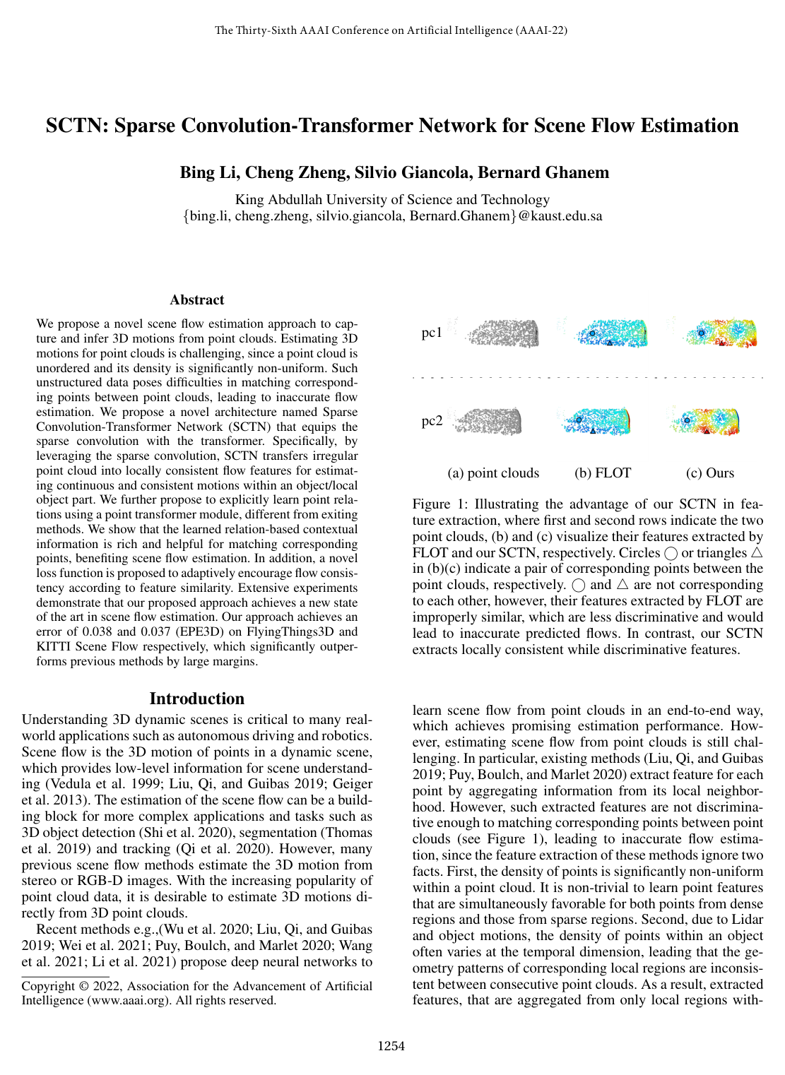
Understanding 3D motion in dynamic environments is critical for high-stakes technologies such as autonomous vehicles and robotics. Scene flow estimation predicts the 3D movement of points between consecutive sensor captures, serving as a vital foundation for object detection, segmentation, and tracking. However, estimating motion directly from 3D point clouds is challenging because sensor data is irregular, unordered, non-uniform in density, and constantly shifting over time. Existing deep learning methods struggle to extract distinct features across sparse and dense areas, leading to inaccurate point matching and poor generalization when moving from synthetic training datasets to real-world environments.

The article evaluates a novel architecture named the Sparse Convolution-Transformer Network (SCTN) designed to resolve these limitations. The primary objective is to demonstrate that combining voxel-based sparse convolutions with a transformer mechanism and a feature-aware consistency loss significantly improves the accuracy, smoothness, and transferability of 3D motion estimation.

To achieve this, the approach pairs a voxelization and interpolation module, which converts irregular point clouds into smooth local features, with a global point transformer module that explicitly captures long-range relationships across the entire scene. The framework also introduces a feature-aware spatial consistency loss that uses a stop-gradient structure during training to enforce locally smooth motion predictions without degrading feature representations. The model was trained on the synthetic FlyingThings3D dataset consisting of over 19,000 point cloud pairs and evaluated across both synthetic test scenes and 142 real-world sensor scans from the KITTI benchmark without any real-world fine-tuning.

The findings show that SCTN establishes a new performance standard across all primary benchmarks. On the synthetic FlyingThings3D benchmark, SCTN achieved a 3D end-point error of 0.038 meters, outperforming leading approaches like FLOT and PointPWC by 26.9% and 35.5% in error reduction, respectively. When transferred directly to the real-world KITTI dataset without fine-tuning, the model achieved an error of 0.037 meters, reducing error by 33.9% relative to FLOT and achieving a strict accuracy of 87.3%. In addition, the model achieved faster inference times, running in approximately 243 milliseconds per frame compared to 389 milliseconds for FLOT on standard hardware.

These results demonstrate that explicitly learning global context alongside smoothed local features substantially reduces errors caused by non-uniform data density and real-world domain shifts. For engineering and technology leaders, adopting this architecture improves perception reliability and safety margins in dynamic environments while lowering runtime latency, making direct point-cloud motion tracking more practical for real-time robotic systems.

Organizations developing 3D perception pipelines should consider integrating SCTN principles—specifically combining voxel smoothing with transformer-based relation modeling—into their existing motion tracking workflows. To build further operational confidence, teams should conduct pilot deployments on target hardware under challenging edge-case conditions, such as adverse weather, high-speed travel, and heavily occluded environments. While the reported results are highly robust across the standard benchmarks evaluated, stakeholders should note that the system relies on preprocessing steps such as ground-point removal and fixed-depth filters, meaning performance may vary in operational settings with unconstrained ranges and raw sensor noise.

Cover for SCTN: Sparse Convolution-Transformer Network for Scene Flow Estimation

Abstract

We propose a novel scene flow estimation approach to cap- ture and infer 3D motions from point clouds. Estimating 3D motions for point clouds is challenging, since a point cloud is unordered and its density is significantly non-uniform. Such unstructured data poses difficulties in matching correspond- ing points between point clouds, leading to inaccurate flow estimation. We propose a novel architecture named Sparse Convolution-Transformer Network (SCTN) that equips the sparse convolution with the transformer. Specifically, by leveraging the sparse convolution, SCTN transfers irregular point cloud into locally consistent flow features for estimat- ing continuous and consistent motions within an object/local object part. We further propose to explicitly learn point rela- tions using a point transformer module, different from exiting methods. We show that the learned relation-based contextual information is rich and helpful for matching corresponding points, benefiting scene flow estimation. In addition, a novel loss function is proposed to adaptively encourage flow consis- tency according to feature similarity. Extensive experiments demonstrate that our proposed approach achieves a new state of the art in scene flow estimation. Our approach achieves an error of 0.038 and 0.037 (EPE3D) on FlyingThings3D and KITTI Scene Flow respectively, which significantly outper- forms previous methods by large margins.

Table of Contents

  • Introduction
  • Related Work
  • Methodology
  • Voxelization-Interpolation Based Feature Extraction
  • Point Transformer Based Feature Extraction
  • Flow Prediction
  • Training Losses
  • Experiments
  • Quantitative Evaluation
  • Qualitative Evaluation
  • Ablation Study
  • Conclusion
  • Acknowledgments
  • References

Knowls

  1. Knowl 1 — SCTN Architecture and Correlation-Based Scene Flow Estimation

    model/method

    Sparse Convolution-Transformer Network (SCTN) estimates 3D scene flow vectors ui∈R3u_i \in \mathbb{R}^3 for each point pitp_i^t in a source point cloud Pt={pit}i=1nP⊂R3P^t = \{p_i^t\}_{i=1}^{n_P} \subset \mathbb{R}^3 towards a target point cloud Pt+1={pjt+1}j=1nP⊂R3P^{t+1} = \{p_j^{t+1}\}_{j=1}^{n_P} \subset \mathbb{R}^3.

    SCTN processes both point clouds using two complementary feature representations:

    1. Voxelization-Interpolation based Feature Extraction (VIFE) generates locally smooth, density-regularized point features FiSF_i^S.
    2. Point Transformer-based Feature Extraction (PTFE) learns global relational and contextual point features FiRF_i^R.

    The representations are fused per point via residual addition: Fi=FiS+FiRF_i = F_i^S + F_i^R

    Given the fused features FitF_i^t for point pit∈Ptp_i^t \in P^t and Fjt+1F_j^{t+1} for point pjt+1∈Pt+1p_j^{t+1} \in P^{t+1}, SCTN computes the pairwise cosine correlation matrix C(pit,pjt+1)C(p_i^t, p_j^{t+1}): C(pit,pjt+1)=(Fit)TFjt+1∥Fit∥2∥Fjt+1∥2C(p_i^t, p_j^{t+1}) = \frac{(F_i^t)^T F_j^{t+1}}{\|F_i^t\|_2 \|F_j^{t+1}\|_2}

    The resulting correlation matrix is fed into the Sinkhorn optimal transport algorithm to compute soft point correspondences and regress the final 3D scene flow field uu for PtP^t.

  2. Knowl 2 — Voxelization-Interpolation Based Feature Extraction (VIFE)

    model/method

    To alleviate spatial non-uniformity and temporal density variations in raw point clouds, the Voxelization-Interpolation based Feature Extraction (VIFE) module extracts features on a regularized sparse 3D grid and projects them back onto individual points.

    1. Voxelization and Sparse Convolutions: The irregular input points are discretized into 3D voxels (resolution 0.07 m0.07\text{ m}). A 3D U-Net architecture utilizing sparse convolutions (via Minkowski Engine) extracts feature vectors vk∈RCv_k \in \mathbb{R}^C for all non-empty voxels kk.
    2. Inverse Distance Point Feature Interpolation: For each original point coordinate pip_i, the point feature FiS∈RCF_i^S \in \mathbb{R}^C is reconstructed by inverse-distance-weighted interpolation across its KK nearest non-empty voxels Nv(pi)\mathcal{N}_v(p_i):

    FiS=∑k∈Nv(pi)dik−1vk∑k∈Nv(pi)dik−1F_i^S = \frac{\sum_{k \in \mathcal{N}_v(p_i)} d_{ik}^{-1} v_k}{\sum_{k \in \mathcal{N}_v(p_i)} d_{ik}^{-1}}

    where dik=∥pi−ck∥2d_{ik} = \|p_i - c_k\|_2 denotes the Euclidean distance from point pip_i to the center ckc_k of the kk-th closest non-empty voxel.

  3. Knowl 3 — Point Transformer-Based Feature Extraction (PTFE)

    model/method

    To compensate for geometric information loss caused by aggressive voxel downsampling in VIFE, the Point Transformer-based Feature Extraction (PTFE) module captures scene-wide point relationships and contextual semantics via global self-attention across all points in the point cloud PP.

    For each point pjp_j, an absolute positional encoding vector GjG_j is generated via a multilayer perceptron (MLP) ϕ\phi: Gj=ϕ(pj)G_j = \phi(p_j)

    The relational feature FiRF_i^R for point pip_i is computed by aggregating linear projections gv(⋅)g_v(\cdot) of VIFE features FjSF_j^S and positional encodings GjG_j weighted by attention coefficients Ai,jA_{i,j}: FiR=∑j=1nPAi,j⋅gv(FjS,Gj)F_i^R = \sum_{j=1}^{n_P} A_{i,j} \cdot g_v(F_j^S, G_j)

    The attention weight Ai,jA_{i,j} represents the similarity between query point pip_i and key point pjp_j in an embedding space of dimension cac_a, parameterized by learnable projections gqg_q and gkg_k: Ai,j=exp⁡((gq(FiS,Gi))Tgk(FjS,Gj)ca)∑l=1nPexp⁡((gq(FiS,Gi))Tgk(FlS,Gl)ca)A_{i,j} = \frac{\exp\left(\frac{(g_q(F_i^S, G_i))^T g_k(F_j^S, G_j)}{c_a}\right)}{\sum_{l=1}^{n_P} \exp\left(\frac{(g_q(F_i^S, G_i))^T g_k(F_l^S, G_l)}{c_a}\right)}

    Using global attention over all scene points provides long-range contextual cues while relying on absolute positional encodings rather than relative offsets reduces computational overhead.

  4. Knowl 4 — Feature-Aware Spatial Consistency (FSC) Loss with Stop-Gradient

    equation

    The Feature-aware Spatial Consistency (FSC) loss enforces predicted scene flows to be smooth and consistent across neighboring points that exhibit high feature similarity, without requiring ground-truth instance or object segmentation masks:

    Ec=∑i=1N1K∑pj∈N(pi)s(Fi,Fj)⋅∥ui−uj∥2E_c = \sum_{i=1}^N \frac{1}{K} \sum_{p_j \in \mathcal{N}(p_i)} s(F_i, F_j) \cdot \|u_i - u_j\|_2

    where N(pi)\mathcal{N}(p_i) is the local spatial neighborhood of point pip_i containing KK points, uiu_i and uju_j are predicted 3D flow vectors, and the feature similarity function s(Fi,Fj)s(F_i, F_j) is defined as:

    s(Fi,Fj)=1−exp⁡(−FiTFjτ)s(F_i, F_j) = 1 - \exp\left(-\frac{F_i^T F_j}{\tau}\right)

    with temperature hyperparameter τ\tau.

    Stop-Gradient Mechanism: A direct joint optimization of EcE_c causes a degenerate collapse where the network sets features orthogonal (FiTFj=0  ⟹  s(Fi,Fj)=0F_i^T F_j = 0 \implies s(F_i, F_j) = 0). To prevent this, gradients from EcE_c are blocked from propagating into the feature similarity computation branch (stop-gradient), ensuring the loss updates only the flow prediction branch by penalizing flow discrepancies ∥ui−uj∥2\|u_i - u_j\|_2 among feature-similar neighbors.

  5. Knowl 5 — Supervised Training Scheme and Optimization Protocol

    experimental setup

    SCTN is trained end-to-end to minimize a cumulative loss function balancing supervised error and spatial flow consistency:

    E=Es+λEcE = E_s + \lambda E_c

    where λ=0.30\lambda = 0.30, EcE_c is the feature-aware spatial consistency loss, and EsE_s is the supervised L1L_1 flow regression loss computed over non-occluded points:

    Es=∑i=1Nmi∥ui−ui∗∥1E_s = \sum_{i=1}^N m_i \|u_i - u_i^*\|_1

    where ui∗u_i^* is the ground-truth motion vector and mi∈{0,1}m_i \in \{0, 1\} is a binary mask indicating whether point pip_i is non-occluded (mi=1m_i = 1) or occluded (mi=0m_i = 0).

    Training Protocol:

    • Optimizer: Adam with an initial learning rate of 10−310^{-3}, decayed to 10−410^{-4} after the 50th epoch.
    • Schedule: Total 60 epochs on FlyingThings3D. The first 40 epochs are trained solely with the supervised loss EsE_s. The remaining 20 epochs are trained with the combined loss Es+λEcE_s + \lambda E_c.
    • Voxel Resolution: 0.07 m0.07\text{ m} voxel grid size for the sparse convolution modules.
    • Point Sampling: 8,192 points randomly sampled per point cloud, excluding points with depth >35 m> 35\text{ m}.
  6. Knowl 6 — Quantitative Benchmark Comparison on FlyingThings3D and KITTI

    data/table

    SCTN was evaluated against state-of-the-art scene flow methods on the synthetic FlyingThings3D test set (3,824 pairs) and evaluated zero-shot (without fine-tuning) on the real-world KITTI Scene Flow dataset (142 pairs). Evaluation metrics comprise:

    • EPE3D (m): End-point error measuring average L2L_2 distance between predicted and ground-truth flow vectors.
    • Acc3DS: Strict accuracy, the fraction of points with EPE3D<0.05 m\text{EPE3D} < 0.05\text{ m} or relative error <5%< 5\%.
    • Acc3DR: Relaxed accuracy, the fraction of points with EPE3D<0.10 m\text{EPE3D} < 0.10\text{ m} or relative error <10%< 10\%.
    • Outliers: Fraction of points with EPE3D>0.30 m\text{EPE3D} > 0.30\text{ m} or relative error >10%> 10\%.
    Dataset Method EPE3D(m) ↓\downarrow Acc3DS ↑\uparrow Acc3DR ↑\uparrow Outliers ↓\downarrow
    FlyingThings3D FlowNet3D 0.114 0.412 0.771 0.602
    HPLFlowNet 0.080 0.614 0.855 0.429
    PointPWC 0.059 0.738 0.928 0.342
    EgoFlow 0.069 0.670 0.879 0.404
    FLOT 0.052 0.732 0.927 0.357
    SCTN (ours) 0.038 0.847 0.968 0.268
    KITTI FlowNet3D 0.177 0.374 0.668 0.527
    HPLFlowNet 0.117 0.478 0.778 0.410
    PointPWC 0.069 0.728 0.888 0.265
    EgoFlow 0.103 0.488 0.822 0.394
    FLOT 0.056 0.755 0.908 0.242
    SCTN (ours) 0.037 0.873 0.959 0.179

    SCTN improves EPE3D by 26.9% on FlyingThings3D and by 33.9% on KITTI compared to the closest baseline (FLOT), achieving sub-4cm average 3D endpoint errors on both benchmarks.

  7. Knowl 7 — Ablation Analysis of SCTN Architectural Components

    data/table

    An ablation study on the KITTI Scene Flow dataset evaluates the contribution of the Voxelization-Interpolation Feature Extraction (VIFE) module, the Point Transformer Feature Extraction (PTFE) module, and the Feature-aware Spatial Consistency (FSC) loss.

    VIFE PTFE FSC loss EPE3D(m) ↓\downarrow Acc3DS ↑\uparrow
    ✓ 0.045 0.835
    ✓ ✓ 0.042 0.853
    ✓ ✓ 0.040 0.863
    ✓ ✓ ✓ 0.037 0.873
    • The VIFE module alone achieves 0.045 m0.045\text{ m} EPE3D, outperforming prior state-of-the-art models.
    • Integrating the PTFE module onto VIFE reduces EPE3D from 0.045 m0.045\text{ m} to 0.040 m0.040\text{ m} (an 11.1% error reduction), demonstrating the benefit of global point relational context.
    • Adding the FSC loss provides consistent accuracy gains across configurations, reaching the best performance of 0.037 m0.037\text{ m} EPE3D and 0.8730.873 Acc3DS.
  8. Knowl 8 — Inference Latency Comparison of SCTN and FLOT

    data/table

    Runtime efficiency was evaluated on a single NVIDIA GTX 2080Ti GPU with 8,192 input points per point cloud pair, comparing SCTN against its most directly related correlation-based baseline, FLOT.

    Method Runtime (ms)
    FLOT 389.3
    SCTN (ours) 242.7

    Despite incorporating a global point transformer module, SCTN achieves a 37.7% faster inference speed than FLOT due to the computational efficiency of sparse convolutions in VIFE and absolute positional encoding in PTFE.

Coverage note — None. All substantive contributions—including the VIFE module, PTFE module, FSC loss with stop-gradient, overall architecture, training configuration, main benchmark evaluations on FlyingThings3D and KITTI, ablation experiments, and runtime analysis—have been converted into standalone knowls.

References

  1. 1.Black, M. J.; and Anandan, P. 1993. A framework for the robust estimation of optical flow. In ICCV, 231–236. IEEE.
  2. 2.Brox, T.; Bregler, C.; and Malik, J. 2009. Large displacement optical flow. In CVPR, 41–48. IEEE.
  3. 3.Carion, N.; Massa, F.; Synnaeve, G.; Usunier, N.; Kirillov, A.; and Zagoruyko, S. 2020. End-to-end object detection with transformers. In ECCV, 213–229.
  4. 4.Chang, A. X.; Funkhouser, T.; Guibas, L.; Hanrahan, P.; Huang, Q.; Li, Z.; Savarese, S.; Savva, M.; Song, S.; Su, H.; Xiao, J.; Yi, L.; and Yu, F. 2015. ShapeNet: An Information-Rich 3D Model Repository. Technical Report arXiv:1512.03012 [cs.GR], arXiv preprint.
  5. 5.Chen, X.; and He, K. 2020. Exploring Simple Siamese Representation Learning. arXiv:2011.10566.
  6. 6.Chen, Y.; Van Gool, L.; Schmid, C.; and Sminchisescu, C. 2020. Consistency Guided Scene Flow Estimation. In ECCV, 125–141. Springer.
  7. 7.Chizat, L.; Peyre, G.; Schmitzer, B.; and Vialard, F.-X. 2018. Scaling algorithms for unbalanced optimal transport problems. Mathematics of Computation, 87(314): 2563–2609.
  8. 8.Choy, C.; Gwak, J.; and Savarese, v. 2019. 4D Spatio-Temporal ConvNets: Minkowski Convolutional Neural Networks. In CVPR, 3075–3084.
  9. 9.Cuturi, M. 2013. Sinkhorn distances: lightspeed computation of optimal transport. In NeurIPS, volume 2, 4.
  10. 10.Dewan, A.; Caselitz, T.; Tipaldi, G. D.; and Burgard, W. 2016. Rigid scene flow for 3d lidar scans. In IROS, 1765–1770. IEEE.
  11. 11.Dosovitskiy, A.; Fischer, P.; Ilg, E.; Hausser, P.; Hazirbas, C.; Golkov, V.; Van Der Smagt, P.; Cremers, D.; and Brox, T. 2015. Flownet: Learning optical flow with convolutional networks. In ICCV, 2758–2766.
  12. 12.Engel, N.; Belagiannis, V.; and Dietmayer, K. 2020. Point Transformer. arXiv:2011.00931.
  13. 13.Geiger, A.; Lenz, P.; Stiller, C.; and Urtasun, R. 2013. Vision meets robotics: The kitti dataset. The International Journal of Robotics Research, 32(11): 1231–1237.
  14. 14.Gojcic, Z.; Litany, O.; Wieser, A.; Guibas, L. J.; and Birdal, T. 2021. Weakly Supervised Learning of Rigid 3D Scene Flow. In CVPR, 5692–5703.
  15. 15.Gu, X.; Wang, Y.; Wu, C.; Lee, Y. J.; and Wang, P. 2019. HPLFlowNet: Hierarchical Permutohedral Lattice FlowNet for Scene Flow Estimation on Large-scale Point Clouds. In CVPR.
  16. 16.Guo, M.-H.; Cai, J.-X.; Liu, Z.-N.; Mu, T.-J.; Martin, R. R.; and Hu, S.-M. 2021. PCT: Point Cloud Transformer. arXiv:2012.09688.
  17. 17.Horn, B. K.; and Schunck, B. G. 1981. Determining optical flow. Artificial intelligence, 17(1-3): 185–203.
  18. 18.Hu, W.; Pang, J.; Liu, X.; Tian, D.; Chia-Wen, L.; and Anthony, V. 2022. Graph signal processing for geometric data and beyond: Theory and applications. IEEE Trans. Multimedia.
  19. 19.Huguet, F.; and Devernay, F. 2007. A variational method for scene flow estimation from stereo sequences. In ICCV, 1–7. IEEE.
  20. 20.Hui, T.-W.; and Loy, C. C. 2020. LiteFlowNet3: Resolving Correspondence Ambiguity for More Accurate Optical Flow Estimation. In ECCV, 169–184. Springer.
  21. 21.Hui, T.-W.; Tang, X.; and Loy, C. C. 2018. Liteflownet: A lightweight convolutional neural network for optical flow estimation. In CVPR, 8981–8989.
  22. 22.Ilg, E.; Mayer, N.; Saikia, T.; Keuper, M.; Dosovitskiy, A.; and Brox, T. 2017. Flownet 2.0: Evolution of optical flow estimation with deep networks. In CVPR, 2462–2470.
  23. 23.Ilg, E.; Saikia, T.; Keuper, M.; and Brox, T. 2018. Occlusions, motion and depth boundaries with a generic network for disparity, optical flow or scene flow estimation. In ECCV, 614–630.
  24. 24.Jiang, H.; Sun, D.; Jampani, V.; Lv, Z.; Learned-Miller, E.; and Kautz, J. 2019. Sense: A shared encoder network for scene-flow estimation. In ICCV, 3195–3204.
  25. 25.Kingma, D. P.; and Ba, J. 2014. Adam: A method for stochastic optimization. arXiv preprint arXiv:1412.6980.
  26. 26.Kittenplon, Y.; Eldar, Y. C.; and Raviv, D. 2021. FlowStep3D: Model Unrolling for Self-Supervised Scene Flow Estimation. In CVPR, 4114–4123.
  27. 27.Lei, H.; Akhtar, N.; and Mian, A. 2020. Spherical kernel for efficient graph convolution on 3d point clouds. TPAMI.
  28. 28.Li, R.; Lin, G.; He, T.; Liu, F.; and Shen, C. 2021. HCRF-Flow: Scene Flow From Point Clouds With Continuous High-Order CRFs and Position-Aware Flow Embedding. In Proceedings of the IEEE/CVF Conference on Computer Vision and Pattern Recognition (CVPR), 364–373.
  29. 29.Li, Y.; Bu, R.; Sun, M.; Wu, W.; Di, X.; and Chen, B. 2018. PointCNN: Convolution on χ-transformed points. In NeurIPS, 828–838.
  30. 30.Liu, X.; Qi, C. R.; and Guibas, L. J. 2019. FlowNet3D: Learning Scene Flow in 3D Point Clouds. In CVPR.
  31. 31.Liu, Z.; Hu, H.; Cao, Y.; Zhang, Z.; and Tong, X. 2020. A closer look at local aggregation operators in point cloud analysis. In ECCV, 326–342. Springer.
  32. 32.Liu, Z.; Tang, H.; Lin, Y.; and Han, S. 2019. Point-Voxel CNN for Efficient 3D Deep Learning. In NeurIPS.
  33. 33.Ma, W.-C.; Wang, S.; Hu, R.; Xiong, Y.; and Urtasun, R. 2019. Deep Rigid Instance Scene Flow. In CVPR.
  34. 34.Mayer, N.; Ilg, E.; Hausser, P.; Fischer, P.; Cremers, D.; Dosovitskiy, A.; and Brox, T. 2016. A large dataset to train convolutional networks for disparity, optical flow, and scene flow estimation. In CVPR, 4040–4048.
  35. 35.Menze, M.; Heipke, C.; and Geiger, A. 2018. Object Scene Flow. JPRS.
  36. 36.Mittal, H.; Okorn, B.; and Held, D. 2020. Just Go With the Flow: Self-Supervised Scene Flow Estimation. In CVPR.
  37. 37.N.Mayer; E.Ilg; P.Hausser; P.Fischer; D.Cremers; ¨A.Dosovitskiy; and T.Brox. 2016a. A Large Dataset to Train Convolutional Networks for Disparity, Optical Flow, and Scene Flow Estimation. In CVPR.
  38. 38.N.Mayer; E.Ilg; P.Hausser; P.Fischer; D.Cremers; ¨A.Dosovitskiy; and T.Brox. 2016b. A Large Dataset to Train Convolutional Networks for Disparity, Optical Flow, and Scene Flow Estimation. In CVPR.
  39. 39.Paszke, A.; Gross, S.; Massa, F.; Lerer, A.; Bradbury, J.; Chanan, G.; Killeen, T.; Lin, Z.; Gimelshein, N.; Antiga, L.; et al. 2019. Pytorch: An imperative style, high-performance deep learning library. arXiv preprint arXiv:1912.01703.
  40. 40.Puy, G.; Boulch, A.; and Marlet, R. 2020. FLOT: Scene Flow on Point Clouds Guided by Optimal Transport. In ECCV.
  41. 41.Qi, C. R.; Su, H.; Mo, K.; and Guibas, L. J. 2017a. Pointnet: Deep learning on point sets for 3d classification and segmentation. In CVPR, 652–660.
  42. 42.Qi, C. R.; Yi, L.; Su, H.; and Guibas, L. J. 2017b. PointNet++: Deep Hierarchical Feature Learning on Point Sets in a Metric Space. In NeurIPS, 5099–5108.
  43. 43.Qi, H.; Feng, C.; Cao, Z.; Zhao, F.; and Xiao, Y. 2020. P2B: Point-to-box network for 3D object tracking in point clouds. In CVPR, 6329–6338.
  44. 44.Quiroga, J.; Brox, T.; Devernay, F.; and Crowley, J. 2014. Dense semi-rigid scene flow estimation from rgbd images. In ECCV, 567–582. Springer.
  45. 45.Ranftl, R.; Bredies, K.; and Pock, T. 2014. Non-local total generalized variation for optical flow estimation. In ECCV, 439–454. Springer.
  46. 46.Ronneberger, O.; Fischer, P.; and Brox, T. 2015. U-net: Convolutional networks for biomedical image segmentation. In MICCAI, 234–241. Springer.
  47. 47.Shi, S.; Guo, C.; Jiang, L.; Wang, Z.; Shi, J.; Wang, X.; and Li, H. 2020. Pv-rcnn: Point-voxel feature set abstraction for 3d object detection. In CVPR, 10529–10538.
  48. 48.Sun, D.; Sudderth, E. B.; and Pfister, H. 2015. Layered RGBD scene flow estimation. In CVPR, 548–556.
  49. 49.Sun, D.; Yang, X.; Liu, M.-Y.; and Kautz, J. 2018. PWC-Net: CNNs for Optical Flow Using Pyramid, Warping, and Cost Volume. In CVPR.
  50. 50.Tang, H.; Liu, Z.; Zhao, S.; Lin, Y.; Lin, J.; Wang, H.; and Han, S. 2020. Searching Efficient 3D Architectures with Sparse Point-Voxel Convolution. In ECCV.
  51. 51.Teed, Z.; and Deng, J. 2020a. RAFT-3D: Scene Flow using Rigid-Motion Embeddings. arXiv preprint arXiv:2012.00726.
  52. 52.Teed, Z.; and Deng, J. 2020b. Raft: Recurrent all-pairs field transforms for optical flow. In ECCV, 402–419. Springer.
  53. 53.Thomas, H.; Qi, C. R.; Deschaud, J.-E.; Marcotegui, B.; Goulette, F.; and Guibas, L. J. 2019. Kpconv: Flexible and deformable convolution for point clouds. In ICCV, 6411–6420.
  54. 54.Tishchenko, I.; Lombardi, S.; Oswald, M. R.; and Pollefeys, M. 2020. Self-Supervised Learning of Non-Rigid Residual Flow and Ego-Motion. arXiv preprint arXiv:2009.10467.
  55. 55.Ushani, A. K.; Wolcott, R. W.; Walls, J. M.; and Eustice, R. M. 2017. A learning approach for real-time temporal scene flow estimation from lidar data. In ICRA, 5666–5673. IEEE.
  56. 56.Vedula, S.; Baker, S.; Rander, P.; Collins, R.; and Kanade, T. 1999. Three-dimensional scene flow. In ICCV, volume 2, 722–729. IEEE.
  57. 57.Vogel, C.; Schindler, K.; and Roth, S. 2013. Piecewise rigid scene flow. In ICCV, 1377–1384.
  58. 58.Wang, H.; Pang, J.; Lodhi, M. A.; Tian, Y.; and Tian, D. 2021. FESTA: Flow Estimation via Spatial-Temporal Attention for Scene Point Clouds. In CVPR, 14173–14182.
  59. 59.Wang, P.-S.; Liu, Y.; Guo, Y.-X.; Sun, C.-Y.; and Tong, X. 2017. O-CNN: Octree-based Convolutional Neural Networks for 3D Shape Analysis. ACM Trans. Graph., 36(4): 72:1–72:11.
  60. 60.Wang, Z.; Li, S.; Howard-Jenkins, H.; Prisacariu, V.; and Chen, M. 2020. FlowNet3D++: Geometric Losses For Deep Scene Flow Estimation. In WACV.
  61. 61.Wedel, A.; Rabe, C.; Vaudrey, T.; Brox, T.; Franke, U.; and Cremers, D. 2008. Efficient dense scene flow from sparse or dense stereo data. In ECCV, 739–751. Springer.
  62. 62.Wei, Y.; Wang, Z.; Rao, Y.; Lu, J.; and Zhou, J. 2021. PV-RAFT: Point-Voxel Correlation Fields for Scene Flow Estimation of Point Clouds. In CVPR.
  63. 63.Weinzaepfel, P.; Revaud, J.; Harchaoui, Z.; and Schmid, C. 2013. DeepFlow: Large displacement optical flow with deep matching. In ICCV, 1385–1392.
  64. 64.Wu, W.; Qi, Z.; and Fuxin, L. 2019. Pointconv: Deep convolutional networks on 3d point clouds. In CVPR, 9621–9630.
  65. 65.Wu, W.; Wang, Z. Y.; Li, Z.; Liu, W.; and Fuxin, L. 2020. PointPWC-Net: Cost Volume on Point Clouds for (Self-) Supervised Scene Flow Estimation. In ECCV, 88–107.
  66. 66.Wu, Z.; Song, S.; Khosla, A.; Yu, F.; Zhang, L.; Tang, X.; and Xiao, J. 2015. 3d shapenets: A deep representation for volumetric shapes. In CVPR, 1912–1920.
  67. 67.Xie, S.; Gu, J.; Guo, D.; Qi, C. R.; Guibas, L.; and Litany, O. 2020. PointContrast: Unsupervised Pre-training for 3D Point Cloud Understanding. In ECCV.
  68. 68.Zach, C.; Pock, T.; and Bischof, H. 2007. A duality based approach for realtime tv-l 1 optical flow. In Joint pattern recognition symposium, 214–223. Springer.
  69. 69.Zhang, Z.; Hua, B.-S.; and Yeung, S.-K. 2019. ShellNet: Efficient Point Cloud Convolutional Neural Networks Using Concentric Shells Statistics. In ICCV.
  70. 70.Zhao, H.; Jia, J.; and Koltun, V. 2020. Exploring Self-Attention for Image Recognition. In CVPR.
  71. 71.Zhao, H.; Jiang, L.; Jia, J.; Torr, P.; and Koltun, V. 2021. Point Transformer. In ICCV.
  72. 72.Zhu, X.; Su, W.; Lu, L.; Li, B.; Wang, X.; and Dai, J. 2021. Deformable DETR: Deformable Transformers for End-to-End Object Detection. In ICLR.

Citation

MLA
Li, B., et al. “SCTN: Sparse Convolution-Transformer Network for Scene Flow Estimation”. arXiv, 2021, http://arxiv.org/abs/2105.04447v4.
APA
Li, B., Zheng, C., Giancola, S., & Ghanem, B. (2021). SCTN: Sparse Convolution-Transformer Network for Scene Flow Estimation. arXiv. http://arxiv.org/abs/2105.04447v4
Chicago
Li, B., C. Zheng, S. Giancola, and B. Ghanem. 2021. “SCTN: Sparse Convolution-Transformer Network for Scene Flow Estimation”. arXiv. http://arxiv.org/abs/2105.04447v4.
Harvard
Li, B. et al. (2021) “SCTN: Sparse Convolution-Transformer Network for Scene Flow Estimation”, arXiv [Preprint]. Available at: http://arxiv.org/abs/2105.04447v4.
Vancouver
1. Li B, Zheng C, Giancola S, Ghanem B (2021) SCTN: Sparse Convolution-Transformer Network for Scene Flow Estimation. arXiv

BibTeX

@article{li2021sctn,
  title = {SCTN: Sparse Convolution-Transformer Network for Scene Flow Estimation},
  author = {Li, Bing and Zheng, Cheng and Giancola, Silvio and Ghanem, Bernard},
  year = {2021},
  journal = {arXiv},
  url = {http://arxiv.org/abs/2105.04447v4},
  eprint = {2105.04447}
}
Metadata:arXiv

Access the Paper

This paper is available from its original source. Click below to access the PDF.

Open PDF