Higher-order organization of complex networks

Austin R. BensonDavid F. GleichJure Leskovec

article2016Science1,376 citations

Develops a scalable, mathematically rigorous framework for clustering complex networks based on higher-order subgraph patterns rather than simple edges, exposing functional modular structures in massive biological, neural, and transportation systems.

Listen

Complex real-world systems across biology, engineering, neuroscience, and social sciences are routinely modeled as networks. Traditional network analysis primarily groups nodes based on simple pairwise links, which fails to capture higher-order building blocks such as triangular patterns, feedback loops, and multi-node pathways. This gap limits our ability to detect functional modules, control mechanisms, and structural roles in complex systems.

The article develops and demonstrates a generalized computational framework that clusters networks using higher-order connectivity patterns, known as network motifs. It aims to prove theoretical optimality guarantees for these higher-order clusters while scaling efficiently to massive, billion-edge networks.

The approach generalizes spectral graph partitioning to higher-order structures by forming a motif adjacency matrix based on how frequently nodes co-occur within specified subgraphs. It then computes an eigenvector of the associated normalized matrix and sweeps across the resulting node ordering to identify clusters that minimize motif conductance. The authors validated the method across 16 large-scale real-world datasets spanning social, web, transportation, biological, and ecological systems, with graph sizes up to nearly two billion edges and motifs up to size nine.

The evaluation yielded several critical findings. First, for three-node motifs, the framework provides a rigorous mathematical guarantee known as a Cheeger inequality, proving that the discovered clusters are within a quadratic factor of theoretical optimality. Second, in real-world benchmark networks, the computational time scaled at approximately m^1.2 with respect to the number of edges m, vastly outperforming theoretical worst-case limits of m^1.5 and processing multi-billion-edge graphs in several hours. Third, higher-order clustering uncovered functional organization that pairwise methods missed entirely, such as isolating a 20-neuron regulatory circuit in C. elegans, achieving 97% accuracy in identifying functional modules in yeast gene regulation (versus 68–82% for standard techniques), and categorizing Florida Bay food web compartments with 61% accuracy (compared to 48–53% for edge-based methods). Finally, when applied to North American air transportation networks, the method cleanly separated hub hierarchy and geographic layout, whereas traditional edge-based methods conflated large hubs with minor regional nodes.

These findings imply that higher-order motifs reveal critical system-level behaviors—such as information flow, control dynamics, and topological anomalies—that edge-based clustering obscures. For organizations managing large-scale networks, this approach reduces the risk of misidentifying core operational hubs, improves anomaly detection in social and web graphs, and delivers higher precision for biological discovery without requiring excessive computational resources.

Decision-makers and analysts should adopt higher-order clustering when simple pairwise methods produce overly broad, spatially biased, or functionally ambiguous groupings. In applications where the key motif is known in advance, organizations should target that specific pattern; when the structure is unknown, analysts should evaluate multiple motifs to uncover the network's governing modular architecture. Future work should focus on automating the selection of optimal motifs for uncharacterized domains and deploying distributed, parallel pipelines to handle growing streaming datasets.

Confidence in these findings is high due to the combination of formal mathematical optimality proofs and extensive empirical testing across diverse real-world domains. Users should note, however, that while three-node motif clustering provides strict Cheeger guarantees, clusters based on motifs with four or more nodes optimize a penalized conductance approximation rather than an exact quadratic bound.

Purdue University Stanford University clustering algorithms complex networks engineering higher-order organization complex networks network motifs

arXiv: 1612.08447 arbenson/higher-order-organization-matlab

Paper: Community detection in graphs, Santo Fortunato (2009). Provides a comprehensive foundation of classic community detection and spectral graph partitioning algorithms before exploring higher-order subgraph clustering.
Paper: Learning with Hypergraphs: Clustering, Classification, and Embedding, Dengyong Zhou et al. (2006). Introduces foundational spectral hypergraph partitioning and hypergraph Laplacians that generalize pairwise network clustering to multi-node interactions.
Paper: Kernel k-means: spectral clustering and normalized cuts, Inderjit S. Dhillon et al. (2004). Establishes the mathematical equivalence between normalized graph cuts and spectral clustering that underpins optimal graph partitioning theory.
Paper: Stochastic blockmodels and community structure in networks, Brian Karrer et al. (2010). Develops the degree-corrected stochastic blockmodel, highlighting how node-level connectivity variations influence network group discovery.
Paper: Defining and evaluating network communities based on ground-truth, Jaewon Yang et al. (2012). Systematically defines and evaluates axiomatic community detection metrics on large-scale ground-truth network benchmarks.
Paper: Self-Tuning Spectral Clustering, Lihi Zelnik-Manor et al. (2004). Presents key spectral clustering mechanisms and eigenvector projection methods used for partitioning complex relational data.

Paper: Networks beyond pairwise interactions: structure and dynamics, Federico Battiston et al. (2020). Extends the study of higher-order network motifs to a comprehensive framework of generalized hypergraphs, simplicial complexes, and non-pairwise dynamics.
Paper: Weisfeiler and Leman Go Neural: Higher-Order Graph Neural Networks, Christopher Morris et al. (2019). Generalizes higher-order structural motifs into deep learning by developing k-order graph neural networks based on the Weisfeiler-Leman hierarchy.
Paper: Hypergraph Neural Networks, Yifan Feng et al. (2018). Applies higher-order relational modeling to deep graph learning by formulating hyperedge convolutions that capture multi-entity correlations.
Paper: From Louvain to Leiden: guaranteeing well-connected communities, Vincent Traag et al. (2018). Continues the study of scalable and mathematically guaranteed community discovery by introducing the Leiden algorithm to enforce internally connected clusters.
Paper: Hierarchical graph representation learning with differentiable pooling, Rex Ying et al. (2018). Leverages hierarchical network clustering to perform end-to-end differentiable graph coarsening in neural networks.
Paper: Community detection and stochastic block models: recent developments, Emmanuel Abbe (2017). Establishes sharp statistical and computational phase transition limits for community detection recovery in structured networks.
Paper: Design and analysis of experiments in networks: Reducing bias from interference, Dean Eckles et al. (2017). Utilizes graph clustering and triangle-dense subgraphs to mitigate network interference bias in randomized experiments.

Cover for Higher-order organization of complex networks

Abstract

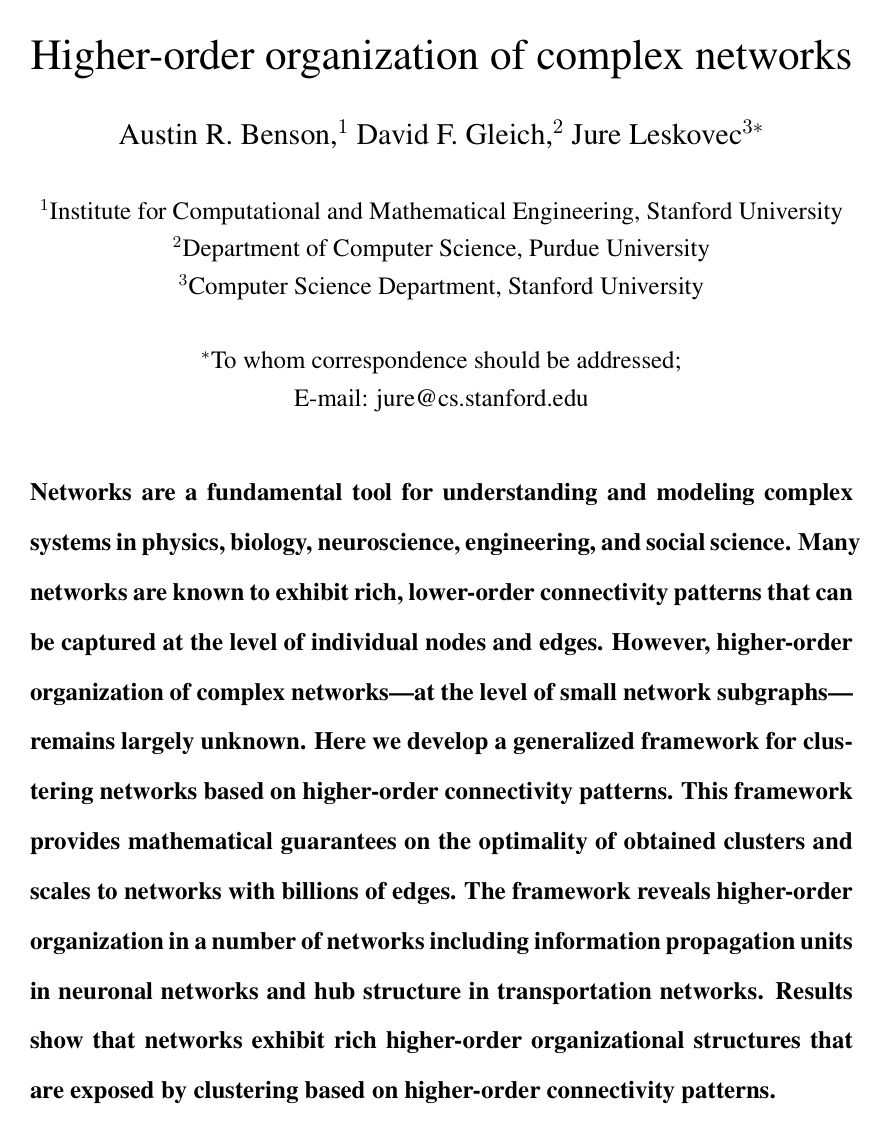
Networks are a fundamental tool for understanding and modeling complex systems in physics, biology, neuroscience, engineering, and social science. Many networks are known to exhibit rich, lower-order connectivity patterns that can be captured at the level of individual nodes and edges. However, higher-order organization of complex networks---at the level of small network subgraphs---remains largely unknown. Here we develop a generalized framework for clustering networks based on higher-order connectivity patterns. This framework provides mathematical guarantees on the optimality of obtained clusters and scales to networks with billions of edges. The framework reveals higher-order organization in a number of networks including information propagation units in neuronal networks and hub structure in transportation networks. Results show that networks exhibit rich higher-order organizational structures that are exposed by clustering based on higher-order connectivity patterns.

Topics

clustering algorithms complex networks engineering information propagation network architecture social sciences

Keywords

higher-order organization complex networks network motifs higher-order connectivity patterns motif adjacency graph clustering higher-order clustering method hypergraph partitioning structural motifs

S1 Derivation and analysis of the motif-based spectral clustering method
S1.1 Review of the graph Laplacian for weighted, undirected graphs
S1.2 Definition of network motifs
S1.3 Definition of motif conductance
S1.4 Definition of the motif adjacency matrix and motif Laplacian
S1.5 Algorithm for finding a single cluster
S1.6 Motif Cheeger inequality for network motifs with three nodes
S1.7 Discussion of motif Cheeger inequality for network motifs with four or more nodes
S1.8 Methods for simultaneously finding multiple clusters
S1.9 Extensions of the method for simultaneously analyzing several network motifs
S1.10 Extensions of the method to signed, colored, and weighted motifs
S1.11 Connections to directed graph partitioning
S1.12 Connections to hypergraph partitioning
S2 Computational complexity and scalability of the method
S2.1 Analysis of computational complexity
S2.2 Experimental results on triangular motifs
S2.3 Experimental results on kk-cliques
S3 Matrix-based interpretation of the motif-weighted adjacency matrix
S4 Alternative clustering algorithms for evaluation
S5 Details and comparison against existing methods for the C. elegans network
S5.1 Connected components of the motif adjacency matrices
S5.2 Comparison of bi-fan motif cluster to clusters found by existing methods
S6 Details and comparison against existing methods for the transportation reachability network
S6.1 Methods for spectral embeddings
S6.2 Comparison of motif-based embedding to other embeddings
S7 Additional case studies
S7.1 Motif M6M_{6} in the Florida Bay food web
S7.1.1 Identifying higher-order modular organization
S7.1.2 Analysis of higher-order modular organization
S7.1.3 Connected components of the motif adjacency matrices
S7.2 Coherent feedforward loops in the S. cerevisiae transcriptional regulation network
S7.2.1 Connected components of the adjacency matrices
S7.2.2 Comparison against existing methods
S7.3 Motif M6M_{6} in the English Wikipedia article network
S7.4 Motif M6M_{6} in the Twitter follower network
S7.5 Motif M7M_{7} in the Stanford web graph
S7.6 Semi-cliques in collaboration networks
S8 Data availability
References and Notes

Knowls

Knowl 1 — Network Motifs and Motif Conductance
definition
Let $G = (V, E)$ be a directed or undirected unweighted graph with adjacency matrix $A$ . A network motif on $k$ nodes is defined as a pair $(B, \mathcal{A})$ , where $B \in \{0, 1\}^{k \times k}$ represents the binary adjacency matrix of the motif subgraph pattern and $\mathcal{A} \subseteq \{1, 2, \dots, k\}$ is a subset of anchor nodes. When $\mathcal{A} = \{1, 2, \dots, k\}$ , the motif is called a simple motif; when $\mathcal{A} \subset \{1, 2, \dots, k\}$ , it is an anchored motif.

The set of motif instances in $G$ , denoted $M(B, \mathcal{A})$ , consists of pairs $(\text{set}(v), \text{set}(\chi_\mathcal{A}(v)))$ for all ordered $k$ -tuples $v = (v_1, \dots, v_k) \in V^k$ of distinct nodes whose induced subgraph adjacency matrix $A_v$ equals $B$ , where $\chi_\mathcal{A}(v)$ selects the tuple entries indexed by $\mathcal{A}$ and $\text{set}(\cdot)$ maps an ordered tuple to an unordered set.

For any non-empty subset of nodes $S \subset V$ with complement $\bar{S} = V \setminus S$ , the motif cut $\text{cut}_M(S, \bar{S})$ counts the number of motif instances whose anchor nodes are split across the partition: $\text{cut}_M(S, \bar{S}) = \sum_{(v, \chi_\mathcal{A}(v)) \in M} \mathbf{1}(\exists i, j \in \chi_\mathcal{A}(v) \text{ such that } i \in S, j \in \bar{S})$

The motif volume $\text{vol}_M(S)$ counts the total number of anchor node instances residing in $S$ : $\text{vol}_M(S) = \sum_{(v, \chi_\mathcal{A}(v)) \in M} \sum_{i \in \chi_\mathcal{A}(v)} \mathbf{1}(i \in S)$

The motif conductance $\phi_M(S)$ with respect to motif $M$ is defined as: $\phi_M(S) = \frac{\text{cut}_M(S, \bar{S})}{\min(\text{vol}_M(S), \text{vol}_M(\bar{S}))}$
Knowl 2 — Motif-Based Single Cluster Spectral Graph Partitioning
algorithm
The motif-based spectral clustering algorithm finds a subset of nodes $S \subset V$ that approximately minimizes the motif conductance $\phi_M(S)$ in a directed or undirected graph $G = (V, E)$ for a motif $M = (B, \mathcal{A})$ .
Input: Graph $G = (V, E)$ and motif $M = (B, \mathcal{A})$
Output: A motif-based cluster $S \subset V$
Form the motif adjacency matrix $W_M \in \mathbb{R}^{n \times n}$ with $(W_M)_{ij} = \sum_{(v, \chi_\mathcal{A}(v)) \in M} \mathbf{1}(\{i, j\} \subseteq \chi_\mathcal{A}(v))$ for $i \neq j$ , and $(W_M)_{ii} = 0$
Compute the diagonal degree matrix $D_M$ with $(D_M)_{ii} = \sum_{j=1}^n (W_M)_{ij}$
Compute the normalized motif Laplacian $\mathcal{L}_M = I - D_M^{-1/2} W_M D_M^{-1/2}$
Compute the eigenvector $z$ associated with the second smallest eigenvalue $\lambda_2$ of $\mathcal{L}_M$
Compute the spectral ordering $\sigma = (\sigma_1, \sigma_2, \dots, \sigma_n)$ by sorting the elements of $D_M^{-1/2} z$ in ascending order
for $r = 1$ to $n-1$ :
     $S_r \leftarrow \{\sigma_1, \dots, \sigma_r\}$
    Compute motif conductance $\phi_M(S_r) = \text{cut}_M(S_r, \bar{S}_r) / \min(\text{vol}_M(S_r), \text{vol}_M(\bar{S}_r))$
$S \leftarrow \arg\min_{S_r} \phi_M(S_r)$
if $|S| \le |V \setminus S|$ :
    return $S$
else:
    return $V \setminus S$
The algorithm reduces motif-based partitioning to standard spectral graph partitioning on the weighted graph $G_M = (V, W_M)$ . Sorting takes $O(n \log n)$ time, and the sweep cut evaluates $n-1$ prefix sets in linear time after forming $W_M$ and computing the Fiedler vector $z$ .
Knowl 3 — Equivalence of Three-Anchor Motif Conductance to Weighted Graph Conductance
theoretical result
Let $G = (V, E)$ be a directed or undirected unweighted graph and let $M = (B, \mathcal{A})$ be any motif with exactly three anchor nodes ( $|\mathcal{A}| = 3$ ). Let $W_M$ be the motif adjacency matrix whose entries $(W_M)_{ij}$ record the number of motif instances containing both nodes $i$ and $j$ in their anchor set for $i \neq j$ , and let $G_M = (V, W_M)$ denote the corresponding weighted undirected graph.

For any node subset $S \subset V$ and its complement $\bar{S} = V \setminus S$ , the motif cut and motif volume satisfy: $\text{cut}_M(S, \bar{S}) = \frac{1}{2} \text{cut}^{(G_M)}(S, \bar{S})$ $\text{vol}_M(S) = \frac{1}{2} \text{vol}^{(G_M)}(S)$

Consequently, the motif conductance on the original graph $G$ is identically equal to the standard graph conductance on the weighted graph $G_M$ : $\phi_M(S) = \phi^{(G_M)}(S)$
Knowl 4 — Motif Cheeger Inequality for Three-Anchor Motifs
theoretical result
Let $G = (V, E)$ be a graph and let $M = (B, \mathcal{A})$ be a motif with $|\mathcal{A}| = 3$ . Let $\phi^* = \min_{S' \subset V} \phi_M(S')$ denote the optimal motif conductance over all non-trivial subsets of $V$ .

Let $\mathcal{L}_M = I - D_M^{-1/2} W_M D_M^{-1/2}$ be the normalized motif Laplacian constructed from the motif adjacency matrix $W_M$ , and let $\lambda_2$ be its second smallest eigenvalue. The cluster $S$ obtained by the motif spectral sweep-cut procedure satisfies the motif Cheeger inequality: $\phi_M(S) \le 4 \sqrt{\phi^*}$ $\phi^* \ge \frac{\lambda_2}{2}$

This guarantees that the motif-based spectral clustering algorithm finds a cluster within a quadratic factor of the globally optimal motif conductance, while $\lambda_2 / 2$ provides a computable lower bound on the optimal motif conductance.
Knowl 5 — Penalized Conductance Relation for Four-Anchor Motifs
theoretical result
For motifs $M = (B, \mathcal{A})$ with four anchor nodes ( $|\mathcal{A}| = 4$ ), the binary indicator function for cutting a motif instance across a partition $(S, \bar{S})$ is quartic rather than quadratic. Consequently, the weighted graph Laplacian formulation on $W_M$ penalizes $2/2$ node splits more heavily than $3/1$ splits.

For any subset $S \subset V$ , the motif cut and weighted graph cut are related by: $\text{cut}_M(S, \bar{S}) = \frac{1}{3} \text{cut}^{(G_M)}(S, \bar{S}) - \frac{1}{3} \sum_{(v, \{i,j,k,l\}) \in M} \mathbf{1}(\text{exactly two of } i, j, k, l \in S)$

Because $\text{vol}_M(S) = \frac{1}{3} \text{vol}^{(G_M)}(S)$ , the motif conductance relates to the weighted graph conductance $\phi^{(G_M)}(S)$ by: $\phi_M(S) = \phi^{(G_M)}(S) - \frac{\sum_{(v, \{i,j,k,l\}) \in M} \mathbf{1}(\text{exactly two of } i, j, k, l \in S)}{\text{vol}^{(G_M)}(S)}$

Thus, spectral partitioning on $W_M$ minimizes a penalized version of motif conductance that places an additional penalty on balanced $2/2$ cuts of the four-node anchor sets.
Knowl 6 — Motif-Based Multi-Cluster Spectral Partitioning
algorithm
To partition a network into $k > 2$ disjoint clusters based on higher-order motif structure, spectral embedding followed by $k$ -means clustering or recursive bi-partitioning is used.
Input: Directed or undirected graph $G = (V, E)$ , motif $M = (B, \mathcal{A})$ , number of clusters $k$
Output: $k$ disjoint clusters $C_1, C_2, \dots, C_k$
Form the motif adjacency matrix $W_M$ where $(W_M)_{ij} = \sum_{(v, \chi_\mathcal{A}(v)) \in M} \mathbf{1}(\{i, j\} \subseteq \chi_\mathcal{A}(v))$ for $i \neq j$
Compute diagonal degree matrix $D_M$ with $(D_M)_{ii} = \sum_{j=1}^n (W_M)_{ij}$
Compute eigenvectors $z_1, z_2, \dots, z_k$ associated with the $k$ smallest eigenvalues of $\mathcal{L}_M = I - D_M^{-1/2} W_M D_M^{-1/2}$
Form the embedding matrix $Z = [z_1, z_2, \dots, z_k] \in \mathbb{R}^{n \times k}$
Construct matrix $Y \in \mathbb{R}^{n \times k}$ with normalized rows: $Y_{ij} = Z_{ij} / \sqrt{\sum_{l=1}^k Z_{il}^2}$
Assign each node $i$ to a cluster $C_1, \dots, C_k$ by running $k$ -means on the row vectors of $Y$
return $C_1, C_2, \dots, C_k$
Alternatively, recursive bi-partitioning applies the single-cluster sweep-cut algorithm repeatedly to the largest remaining cluster until $k$ clusters are formed.
Knowl 7 — Matrix Formulations of Motif Adjacency for Directed Triangular Motifs
model/method
For directed, unweighted graphs $G$ with binary adjacency matrix $A$ , the motif adjacency matrix $W_M$ for each of the seven three-node simple motifs ( $M_1$ through $M_7$ ) can be computed directly using sparse matrix multiplications and Hadamard (entrywise) products $\circ$ .

Let $B = A \circ A^T$ represent the adjacency matrix of bidirectional edges and $U = A - B$ represent the adjacency matrix of unidirectional edges. The matrix $W_M$ is computed via an intermediate matrix $C$ :
- Motif $M_1$ (directed 3-cycle): $C = (U \cdot U) \circ U^T$ , with $W_M = C + C^T$
- Motif $M_2$ : $C = (B \cdot U) \circ U^T + (U \cdot B) \circ U^T + (U \cdot U) \circ B$ , with $W_M = C + C^T$
- Motif $M_3$ : $C = (B \cdot B) \circ U + (B \cdot U) \circ B + (U \cdot B) \circ B$ , with $W_M = C + C^T$
- Motif $M_4$ (bidirectional triangle): $C = (B \cdot B) \circ B$ , with $W_M = C$
- Motif $M_5$ (feedforward loop): $C = (U \cdot U) \circ U + (U \cdot U^T) \circ U + (U^T \cdot U) \circ U$ , with $W_M = C + C^T$
- Motif $M_6$ : $C = (U \cdot B) \circ U + (B \cdot U^T) \circ U^T + (U^T \cdot U) \circ B$ , with $W_M = C$
- Motif $M_7$ : $C = (U^T \cdot B) \circ U^T + (B \cdot U) \circ U + (U \cdot U^T) \circ B$ , with $W_M = C$
Knowl 8 — Framework Extensions to Multi-Motif, Signed, Colored, and Weighted Networks
model/method
The motif-based spectral clustering framework generalizes across multiple network and motif variations:
1. Multiple Motifs: To cluster simultaneously on $q$ different motif sets $M_1, \dots, M_q$ with non-negative weights $\alpha_1, \dots, \alpha_q$ , the composite motif adjacency matrix is formed as: $W_M = \sum_{j=1}^q \alpha_j W_{M_j}$ When all $M_j$ have three anchor nodes, linearity preserves the exact motif Cheeger inequality for the combined weighted conductance.
2. Weighted Motifs: If each motif instance has an associated non-negative weight $\omega(v, \chi_\mathcal{A}(v))$ , entries of $W_M$ are computed as: $(W_M)_{ij} = \sum_{(v, \chi_\mathcal{A}(v)) \in M} \omega(v, \chi_\mathcal{A}(v)) \mathbf{1}(\{i, j\} \subseteq \chi_\mathcal{A}(v))$
3. Signed and Colored Motifs: For signed networks, the motif pattern matrix $B$ includes positive ( $+$ ) and negative ( $-$ ) edge entries to represent relations such as activation vs. inhibition or friend vs. foe. For colored/labeled networks, $B$ specifies categorical node or edge labels, restricting the counts to instances matching the color configuration.
Knowl 9 — Computational Complexity and Empirical Scaling of Motif Adjacency Construction
empirical result
While worst-case triangle enumeration on general graphs with $m$ edges has computational complexity $\Theta(m^{1.5})$ , empirical evaluation of motif adjacency matrix ( $W_M$ ) construction across 16 real-world directed networks (ranging from 159,000 to nearly 2 billion edges and up to 50.6 million nodes) exhibits scaling of $\Theta(m^{1.2})$ .

A linear regression of $\log(\text{time})$ against $\log(m)$ for all triangular motifs ( $M_1$ through $M_7$ ) yields a combined regression slope of $1.17 \pm 0.09$ (95% confidence interval). For specific motifs, the largest observed empirical regression coefficient is $1.31 \pm 0.19$ (for motif $M_3$ ). For the largest evaluated graph (sk-2005 with 1.93 billion edges), serial computation of $W_M$ required at most 52.8 hours and parallel normalized Laplacian eigenvector computation took 1.62 hours.
Knowl 10 — Disentangling Hub Hierarchy and Geography in Transportation Networks via Anchored Motifs
empirical result
In a North American flight reachability network, spectral embedding using anchored two-hop motifs ( $W_M = S^2$ , where $S$ is the bidirectional flight link adjacency matrix) cleanly separates airport hub hierarchy from geographical coordinates.

The primary spectral coordinate of the normalized motif Laplacian correlates strongly with city metropolitan population (Pearson $r = 0.43 \pm 0.09$ , 99% CI $[0.33, 0.53]$ ), placing major hubs (such as Atlanta, Chicago, and Dallas) at one extreme and non-hubs at the other. The secondary spectral coordinate correlates strongly with longitude (Pearson $r = 0.59 \pm 0.08$ , 99% CI $[-0.66, -0.50]$ ), capturing East-West geography.

In contrast, standard edge-based spectral embedding achieves lower correlations ( $r = 0.11 \pm 0.12$ with population, $r = 0.39 \pm 0.11$ with longitude) and conflates geography and hub structure, placing major hub Atlanta directly adjacent to non-hub Salina.
Knowl 11 — Identification of Modular Control Circuits in C. elegans via Bi-Fan Motifs
empirical result
Applying the motif-based spectral clustering framework with the 4-node "bi-fan" motif to the Caenorhabditis elegans frontal neuronal network (131 neurons, 764 synaptic connections) identifies a 20-neuron functional control module with low bi-fan conductance.

The 20-neuron module contains three ring motor neurons (RMEL, RMER, RMEV), six inner labial sensory neurons (IL2DL, IL2DR, IL2VL, IL2VR, IL2L, IL2R), four URA neurons, and the interneuron RIH. This cluster organizes known pioneers of the nerve ring (RME neurons) as information sources and nictation regulators (IL2 neurons) as information destinations, with RIH acting as an intermediary receiving input from all three RME neurons and outputting to five of six IL2 neurons.

Standard edge-based clustering and 3-node wedge motif ( $M_8$ ) clustering fail to isolate this functional unit, instead bisecting the network into large, purely spatial clusters containing 64 and 68 neurons, respectively.
Knowl 12 — Functional Module Detection in S. cerevisiae Transcriptional Regulation via Signed Feedforward Loops
empirical result
In the Saccharomyces cerevisiae transcriptional regulation network (690 operon nodes, 1082 signed directed regulatory edges), spectral clustering based on four signed coherent feedforward loop (FFL) motifs identifies functional operon modules with 97% classification accuracy.

The motif adjacency matrix disconnects the graph into components corresponding to biological functional units (including drug resistance, cell cycle and mating type switch, methionine biosynthesis, leucine biosynthesis, and nitrogen utilization). Partitioning the largest 18-node component correctly identifies the 5-node "cell cycle and mating type switch" module ({CLN1, CLN2, HO, SPT16, SWI4/SWI6}).

Motif-based clustering coherently assigns all 29 labeled FFL instances (100%) to their respective functional clusters. By comparison, edge-based spectral clustering, Infomap, and the Louvain method coherently cluster 25/29, 23/29, and 23/29 motifs, achieving lower classification accuracies of 82%, 68%, and 76%, respectively.
Knowl 13 — Ecological Compartmentalization of the Florida Bay Food Web via Motif M6
empirical result
In the Florida Bay ecosystem food web (128 compartment nodes, 2106 carbon-exchange edges), clustering based on motif $M_6$ (two mutually preying species competing for a third common prey) reveals modular trophic structures with 61.3% purity and an Adjusted Rand Index (ARI) of 0.3265, outperforming edge-based spectral clustering (48.4% purity, 0.1814 ARI), Infomap (46.8% purity, 0.1592 ARI), and the Louvain method (53.2% purity, 0.2207 ARI).

The clustering resolves four ecological compartments: pelagic fishes, benthic fishes and crabs, sea-floor macroinvertebrates, and microfauna/detritus. The spectral eigenvalue lower bound $\lambda_2 / 2$ for motif $M_6$ is 0.0335 (yielding a found cluster conductance of 0.1200), whereas for motifs $M_5$ and $M_8$ the lower bounds are 0.2195 and 0.2191 (with found conductances of 0.4414 and 0.4145), proving that $M_6$ is uniquely capable of exposing low-conductance higher-order organization in this ecosystem.

Coverage note — Omitted brief secondary case study illustrations on the English Wikipedia hyperlink network, Twitter follower network, and Stanford web / co-authorship graphs, as their underlying methodology and structural insights are fully captured by the included primary case studies (C. elegans, airport reachability, S. cerevisiae, and Florida Bay food web) and the general framework knowls.

References

1.R. Milo, et al., Science 298, 824 (2002).
2.S. Mangan, A. Zaslaver, U. Alon, Journal of molecular biology 334, 197 (2003).
3.J. Yang, J. Leskovec, Proceedings of the IEEE 102, 1892 (2014).
4.P. W. Holland, S. Leinhardt, American Journal of Sociology pp. 492–513 (1970).
5.M. Rosvall, A. V. Esquivel, A. Lancichinetti, J. D. West, R. Lambiotte, Nature communications 5 (2014).
6.N. Pržulj, D. G. Corneil, I. Jurisica, Bioinformatics 20, 3508 (2004).
7.J. Leskovec, K. J. Lang, A. Dasgupta, M. W. Mahoney, Internet Mathematics 6, 29 (2009).
8.Ö. N. Yaveroğlu, et al., Scientific reports 4 (2014).
9.S. Mangan, U. Alon, Proceedings of the National Academy of Sciences 100, 11980 (2003).
10.C. J. Honey, R. Kötter, M. Breakspear, O. Sporns, Proceedings of the National Academy of Sciences 104, 10240 (2007).
11.S. E. Schaeffer, Computer Science Review 1, 27 (2007).
12.Minimizing $\phi_M(S)$ is NP-hard, which follows from the NP-hardness of the traditional definition of conductance (68).
13.See the Supplementary Material.
14.Formally, when the motif has three nodes, the selected cluster $S$ satisfies $\phi_M(S) \le 4\sqrt{\phi_M^*} \le 1$ , where $\phi_M^*$ is the smallest motif conductance of any possible node set $S$ . This inequality is proved in the Supplementary Material.
15.The normalized motif Laplacian matrix is $\mathcal{L}_M = D^{-1/2}(D - W_M)D^{-1/2}$ , where $D$ is a diagonal matrix with the row-sums of $W_M$ on the diagonal ( $D_{ii} = \sum_j (W_M)_{ij}$ ), and $D^{-1/2}$ is the same matrix with the inverse square-roots on the diagonal ( $D_{ii}^{-1/2} = 1/\sqrt{\sum_j (W_M)_{ij}}$ ). The spectral ordering $\sigma$ is the by-value ordering of $D^{-1/2}z$ , where $z$ is the eigenvector corresponding to the second smallest eigenvalue of $\mathcal{L}_M$ , i.e., $\sigma_i$ is the index of $D^{-1/2}z$ with the $i$ th smallest value.
16.C. Seshadhri, A. Pinar, T. G. Kolda, Statistical Analysis and Data Mining: The ASA Data Science Journal 7, 294 (2014).
17.R. Andersen, F. Chung, K. Lang, Proceedings of the 47th Annual IEEE Symposium on Foundations of Computer Science (2006), pp. 475–486.
18.J. J. Whang, I. S. Dhillon, D. F. Gleich, SIAM Data Mining (2015).
19.A. Y. Ng, M. I. Jordan, Y. Weiss, Advances in Neural Information Processing Systems 14 (2002), pp. 849–856.
20.D. Boley, Data Mining and Knowledge Discovery 2, 325 (1998).
21.D. L. Riddle, T. Blumenthal, B. J. Meyer, et al., eds., C. elegans II (Cold Spring Harbor Laboratory Press, 1997), second edn.
22.H. Lee, et al., Nature neuroscience 15, 107 (2012).
23.B. J. Frey, D. Dueck, Science 315, 972 (2007).
24.B. Serrour, A. Arenas, S. Gómez, Computer Communications 34, 629 (2011).
25.T. Michoel, A. Joshi, B. Nachtergaele, Y. Van de Peer, Molecular BioSystems 7, 2769 (2011).
26.A. R. Benson, D. F. Gleich, J. Leskovec, SIAM Data Mining (2015).
27.F. Krzakala, et al., Proceedings of the National Academy of Sciences 110, 20935 (2013).
28.M. Kaiser, C. C. Hilgetag, PLoS Computational Biology 2, e95 (2006).
29.U. Alon, Nature Reviews Genetics 8, 450 (2007).
30.O. Sporns, R. Kötter, PLoS Biology 2, e369 (2004).
31.A. Inokuchi, T. Washio, H. Motoda, Principles of Data Mining and Knowledge Discovery (Springer, 2000), pp. 13–23.
32.F. R. Chung, Proceedings of ICCM (Citeseer, 2007), vol. 2, p. 378.
33.J. R. Lee, S. O. Gharan, L. Trevisan, Journal of the ACM 61, 37 (2014).
34.F. Chung, Annals of Combinatorics 9, 1 (2005).
35.D. Boley, G. Ranjan, Z.-L. Zhang, Linear Algebra and its Applications 435, 224 (2011).
36.F. D. Malliaros, M. Vazirgiannis, Physics Reports 533, 95 (2013).
37.G. Karypis, R. Aggarwal, V. Kumar, S. Shekhar, Very Large Scale Integration (VLSI) Systems, IEEE Transactions on 7, 69 (1999).
38.S. Agarwal, K. Branson, S. Belongie, Proceedings of the 23rd International Conference on Machine Learning (ACM, 2006), pp. 17–24.
39.D. Zhou, J. Huang, B. Schölkopf, Advances in Neural Information Processing Systems 19 (MIT Press, 2006), pp. 1601–1608.
40.J. Rodríguez, Linear and Multilinear Algebra 50, 1 (2002).
41.L. Trevisan, Lecture notes on expansion, sparsest cut, and spectral graph theory, http://www.eecs.berkeley.edu/~luca/books/expanders.pdf. Accessed June 28, 2015.
42.S. Demeyer, et al., PloS ONE 8, e61183 (2013).
43.M. Houbraken, et al., PLoS ONE 9, e97896 (2014).
44.S. Wernicke, IEEE/ACM Transactions on Computational Biology and Bioinformatics 3, 347 (2006).
45.S. Wernicke, F. Rasche, Bioinformatics 22, 1152 (2006).
46.C. R. Aberger, A. Nötzli, K. Olukotun, C. Ré, arXiv preprint arXiv:1503.02368 (2015).
47.M. Latapy, Theoretical Computer Science 407, 458 (2008).
48.J. W. Berry, et al., Proceedings of the 5th Conference on Innovations in Theoretical Computer Science (ACM, New York, NY, USA, 2014), pp. 225–234.
49.D. Marcus, Y. Shavitt, IEEE 30th International Conference on Distributed Computing Systems Workshops (2010), pp. 92–98.
50.N. Chiba, T. Nishizeki, SIAM Journal on Computing 14, 210 (1985).
51.T. Schank, D. Wagner, Experimental and Efficient Algorithms (Springer, 2005), pp. 606–609.
52.L. Becchetti, P. Boldi, C. Castillo, A. Gionis, Proceedings of the 14th ACM SIGKDD international conference on Knowledge discovery and data mining (ACM, 2008), pp. 16–24.
53.J. Cohen, Computing in Science & Engineering 11, 29 (2009).
54.B. N. Parlett, The Symmetric Eigenvalue Problem, vol. 7 (SIAM, 1980).
55.K. J. Maschhoff, D. C. Sorensen, Applied Parallel Computing Industrial Computation and Optimization (Springer, 1996), pp. 478–486.
56.J. Leskovec, A. Krevl, SNAP Datasets: Stanford large network dataset collection, http://snap.stanford.edu/data (2014).
57.P. Boldi, B. Codenotti, M. Santini, S. Vigna, Software: Practice and Experience 34, 711 (2004).
58.P. Boldi, S. Vigna, Proceedings of the 13th International Conference on World Wide Web (ACM, 2004), pp. 595–602.
59.P. Boldi, M. Rosa, M. Santini, S. Vigna, Proceedings of the 20th International Conference on World Wide Web (ACM, 2011), pp. 587–596.
60.P. Boldi, A. Marino, M. Santini, S. Vigna, Proceedings of the companion publication of the 23rd international conference on World wide web companion (International World Wide Web Conferences Steering Committee, 2014), pp. 227–228.
61.A. Azad, A. Buluç, J. R. Gilbert, Proceedings of the IPDPSW, Workshop on Graph Algorithm Building Blocks (GABB) (2015), pp. 804–811.
62.M. Rosvall, C. T. Bergstrom, Proceedings of the National Academy of Sciences 105, 1118 (2008).
63.V. D. Blondel, J.-L. Guillaume, R. Lambiotte, E. Lefebvre, Journal of statistical mechanics: theory and experiment 2008, P10008 (2008).
64.R. E. Ulanowicz, C. Bondavalli, M. S. Egnotovich, Trophic Dynamics in South Florida Ecosystem, FY 97: The Florida Bay Ecosystem, Tech. Rep. CBL 98-123, Chesapeake Biological Laboratory, Solomons, MD (1998).
65.J. Bascompte, C. J. Melián, E. Sala, Proceedings of the National Academy of Sciences of the United States of America 102, 5443 (2005).
66.J. Bascompte, et al., Science 325, 416 (2009).
67.D. B. Stouffer, J. Camacho, W. Jiang, L. A. N. Amaral, Proceedings of the Royal Society of London B: Biological Sciences 274, 1931 (2007).
68.D. Wagner, F. Wagner, Proceedings of the 18th International Symposium on Mathematical Foundations of Computer Science (1993), pp. 744–750.
69.C. D. Manning, P. Raghavan, H. Schütze, et al., Introduction to Information Retrieval, vol. 1 (Cambridge university press Cambridge, 2008).
70.R. Dobrin, Q. K. Beg, A.-L. Barabási, Z. N. Oltvai, BMC bioinformatics 5, 10 (2004).
71.H. Kwak, C. Lee, H. Park, S. Moon, Proceedings of the 19th International Conference on World Wide Web (ACM, 2010), pp. 591–600.
72.T. Chakraborty, N. Ganguly, A. Mukherjee, Advances in Social Networks Analysis and Mining (ASONAM), 2014 IEEE/ACM International Conference on (IEEE, 2014), pp. 130–137.
73.J. Leskovec, J. Kleinberg, C. Faloutsos, ACM Transactions on Knowledge Discovery from Data (TKDD) 1, 2 (2007).
74.R. West, H. S. Paskov, J. Leskovec, C. Potts, Transactions of the Association for Computational Linguistics 2, 297 (2014).
75.J. Leskovec, J. Kleinberg, C. Faloutsos, Proceedings of the eleventh ACM SIGKDD international conference on Knowledge discovery in data mining (ACM, 2005), pp. 177–187.
76.J. Gehrke, P. Ginsparg, J. Kleinberg, ACM SIGKDD Explorations Newsletter 5, 149 (2003).
77.R. Albert, H. Jeong, A.-L. Barabási, Nature 401, 130 (1999).
78.J. Leskovec, L. A. Adamic, B. A. Huberman, ACM Transactions on the Web (TWEB) 1, 5 (2007).
79.J. Leskovec, D. P. Huttenlocher, J. M. Kleinberg, ICWSM (2010).
80.J. Leskovec, J. J. Mcauley, Advances in neural information processing systems (2012), pp. 539–547.
81.L. Takac, M. Zabovsky, International Scientific Conference and International Workshop Present Day Trends of Innovations (2012), pp. 1–6.
82.L. Backstrom, D. Huttenlocher, J. Kleinberg, X. Lan, Proceedings of the 12th ACM SIGKDD international conference on Knowledge discovery and data mining (ACM, 2006), pp. 44–54.
83.J. Yang, J. Leskovec, 2012 IEEE 12th International Conference on Data Mining (IEEE, 2012), pp. 745–754.

Citation

MLA

Benson, A. R., et al. “Higher-order Organization of Complex Networks”. Science, vol. 353, no. 6295, 2016, pp. 163–66, https://doi.org/10.1126/science.aad9029.

APA

Benson, A. R., Gleich, D. F., & Leskovec, J. (2016). Higher-order organization of complex networks. Science, 353(6295), 163–166. https://doi.org/10.1126/science.aad9029

Chicago

Benson, A. R., D. F. Gleich, and J. Leskovec. 2016. “Higher-order Organization of Complex Networks”. Science 353 (6295): 163–66. https://doi.org/10.1126/science.aad9029.

Harvard

Benson, A.R., Gleich, D.F. and Leskovec, J. (2016) “Higher-order organization of complex networks”, Science, 353(6295), pp. 163–166. Available at: https://doi.org/10.1126/science.aad9029.

Vancouver

1. Benson AR, Gleich DF, Leskovec J (2016) Higher-order organization of complex networks. Science 353:163–166

BibTeX

@article{Benson_2016, title={Higher-order organization of complex networks}, volume={353}, ISSN={1095-9203}, url={http://dx.doi.org/10.1126/science.aad9029}, DOI={10.1126/science.aad9029}, number={6295}, journal={Science}, publisher={American Association for the Advancement of Science (AAAS)}, author={Benson, Austin R. and Gleich, David F. and Leskovec, Jure}, year={2016}, month=July, pages={163–166} }

Metadata:Crossref

Source Code

This paper has an official code repository available. Click below to access the source code.

View Repository

Access the Paper

This paper is available from its original source. Click below to access the PDF.

Open PDF

Higher-order organization of complex networks

Abstract

Topics

Keywords

Table of Contents

Knowls

Knowl 1 — Network Motifs and Motif Conductance

Knowl 2 — Motif-Based Single Cluster Spectral Graph Partitioning

Knowl 3 — Equivalence of Three-Anchor Motif Conductance to Weighted Graph Conductance

Knowl 4 — Motif Cheeger Inequality for Three-Anchor Motifs

Knowl 5 — Penalized Conductance Relation for Four-Anchor Motifs

Knowl 6 — Motif-Based Multi-Cluster Spectral Partitioning

Knowl 7 — Matrix Formulations of Motif Adjacency for Directed Triangular Motifs

Knowl 8 — Framework Extensions to Multi-Motif, Signed, Colored, and Weighted Networks

Knowl 9 — Computational Complexity and Empirical Scaling of Motif Adjacency Construction

Knowl 10 — Disentangling Hub Hierarchy and Geography in Transportation Networks via Anchored Motifs

Knowl 11 — Identification of Modular Control Circuits in C. elegans via Bi-Fan Motifs

Knowl 12 — Functional Module Detection in S. cerevisiae Transcriptional Regulation via Signed Feedforward Loops

Knowl 13 — Ecological Compartmentalization of the Florida Bay Food Web via Motif M6

References

Citation

BibTeX

Source Code

Access the Paper