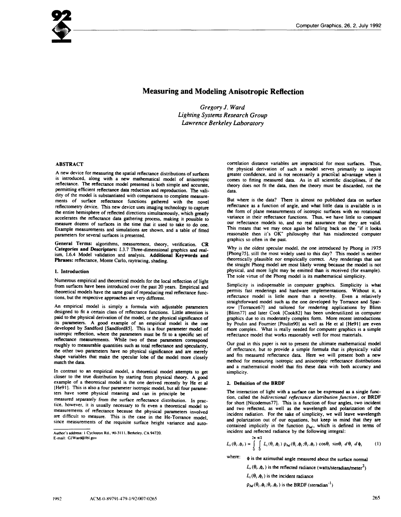
Measuring and modeling anisotropic reflection

G. Ward

article1992SIGGRAPH1,375 citations

Introduces a fast imaging gonioreflectometer that captures entire hemispherical reflectance distributions simultaneously, pairing it with a simple, practical mathematical model for rendering anisotropic surfaces from real-world measurements.

Listen

Accurately simulating how light interacts with complex surfaces remains a persistent challenge in computer graphics and lighting design. Historically, the field has suffered from a critical data shortage because traditional gonioreflectometers—devices used to measure surface reflectance distributions—are mechanically cumbersome, slow, and expensive, often costing thousands of dollars per anisotropic sample. Consequently, practitioners have relied either on computationally prohibitive theoretical formulations or oversimplified empirical equations that violate basic laws of physics, leading to visual inaccuracies and unphysical energy gains in simulations.

The article demonstrates an integrated solution to this problem by introducing a high-speed, cost-effective measurement device alongside a simple, physically valid mathematical reflectance model. Together, these tools evaluate and model both isotropic and anisotropic materials—surfaces that reflect light directionally depending on their orientation—with high computational efficiency.

The authors designed an imaging gonioreflectometer that replaces mechanical detector movement with a half-silvered mirror and a charge-coupled device camera equipped with a fisheye lens, capturing an entire hemisphere of reflected light simultaneously. The resulting empirical model applies an elliptical Gaussian distribution governed by four physically meaningful parameters: diffuse reflectance, specular reflectance, and surface roughness across two perpendicular directions. The authors validated this approach by measuring diverse materials—such as brushed metals, rolled brass, and varnished woods—and fitting the mathematical function to the experimental datasets using least-squares optimization.

The findings establish that the new imaging device reduces data capture times from hours or days to just a few minutes while directly measuring absolute reflectance values. Furthermore, the four-parameter elliptical Gaussian model accurately matches real-world anisotropic measurements and satisfies essential physical requirements, including energy conservation and bidirectional symmetry. When paired with a hybrid rendering method that combines deterministic source tracing with stochastic Monte Carlo sampling, the model eliminates high image noise without increasing computational time relative to standard sampling approaches.

These results provide immediate operational and performance benefits for lighting simulations and computer-generated imagery. Organizations can drastically lower data-acquisition costs, automate material characterization pipelines, and maintain realistic physical rendering without incurring severe memory or rendering overheads. Because the model parameters correspond directly to tangible surface properties, designers can also manually set plausible material behaviors when physical samples are unavailable.

For future development, the article recommends upgrading the measurement hardware with larger, higher-precision optical hemispheres and more tightly collimated light sources to improve measurements at grazing angles and on highly polished surfaces. Practitioners in rendering and optical simulation should adopt normalized, physically valid empirical models and utilize automated fitting routines to expand material databases.

Readers should note current equipment limitations: the prototype struggles with near-grazing incident angles and extremely smooth, mirror-like materials whose sharp reflection peaks exceed the system's collimation limits. Nevertheless, there is high confidence in the demonstrated methodology for rough, brushed, and semi-gloss surfaces across computer graphics and architectural lighting applications.

Lawrence Berkeley National Laboratory Lighting Systems Research Group computational efficiency computer hardware database systems anisotropic reflection BRDF measurement reflectance models

Ward (1992).pdf

Paper: A reflectance model for computer graphics, Robert L. Cook et al. (1981). It introduces a foundational physically based bidirectional reflectance model incorporating microfacet slope distributions and Fresnel equations, which the source builds upon to formulate its four-parameter anisotropic model.
Paper: Models of light reflection for computer synthesized pictures, J. Blinn (1977). It provides the essential optical foundation for microfacet-based specular reflection in computer graphics that underpins subsequent surface reflectance modeling.
Paper: The rendering equation, James T. Kajiya (1986). It formulates the governing rendering equation and Monte Carlo path tracing framework used to integrate and evaluate the source's reflectance model.

Paper: Rendering synthetic objects into real scenes: bridging traditional and image-based graphics with global illumination and high dynamic range photography, P. Debevec (1998). It extends measured real-world reflectance and illumination capture pipelines to seamlessly composite synthetic objects into photographic scenes using global illumination.
Paper: Light field rendering, Marc Levoy et al. (1996). It generalizes image-based directional light capture to full 4D light fields, bypassing explicit analytical BRDF parameter estimation.
Paper: Ref-NeRF: Structured View-Dependent Appearance for Neural Radiance Fields, Dor Verbin et al. (2022). It applies principles of view-dependent specular reflection and surface roughness modeling to modern neural radiance fields.

Cover for Measuring and modeling anisotropic reflection

Abstract

A new device for measuring the spatial reflectance distributions of surfaces is introduced, along with a new mathematical model of anisotropic reflectance. The reflectance model presented is both simple and accurate, permitting efficient reflectance data reduction and reproduction. The validity of the model is substantiated with comparisons to complete measurements of surface reflectance functions gathered with the novel reflectometry device. This new device uses imaging technology to capture the entire hemisphere of reflected directions simultaneously, which greatly accelerates the reflectance data gathering process, making it possible to measure dozens of surfaces in the time that it used to take to do one. Example measurements and simulations are shown, and a table of fitted parameters for several surfaces is presented.

Topics

computational efficiency computer hardware database systems deterministic energy conservation gaussian model image noise isotropic materials lighting conditions optimization

Keywords

anisotropic reflection BRDF measurement reflectance models elliptical Gaussian model anisotropic surfaces Monte Carlo sampling surface reflectance

1. Introduction
2. Definition of the BRDF
3. Measuring the BRDF of a Surface
3.1. An Imaging Gonioreflectometer
3.2. Calibration and Data Reduction
3.3. Measurement Limitations
4. Modeling Anisotropic Reflectance
4.1. The Isotropic Gaussian Model
4.2. The Anisotropic (Elliptical) Gaussian Model
5. Rendering Anisotropic Surfaces
5.1. Stochastic Sampling of Elliptical Gaussian
6. Results
7. Conclusion
8. Acknowledgements
9. References

Knowls

Knowl 1 — Ward Anisotropic Elliptical Gaussian BRDF Model
model/method
The Ward anisotropic bidirectional reflectance distribution function (BRDF) models surface reflection using an elliptical Gaussian distribution of surface slopes with two uncorrelated, orthogonal roughness parameters. The BRDF $\rho_{bd}(\theta_i, \phi_i; \theta_r, \phi_r)$ is defined as:

$\rho_{bd}(\theta_i, \phi_i; \theta_r, \phi_r) = \frac{\rho_d}{\pi} + \frac{\rho_s}{\sqrt{\cos\theta_i \cos\theta_r}} \frac{\exp\left(-\tan^2\delta \left(\frac{\cos^2\phi}{\alpha_x^2} + \frac{\sin^2\phi}{\alpha_y^2}\right)\right)}{4\pi \alpha_x \alpha_y}$

where:
- $\rho_d \in [0, 1]$ is the diffuse reflectance coefficient.
- $\rho_s \in [0, 1]$ is the specular (rough specular / directional diffuse) reflectance coefficient, constrained by $\rho_d + \rho_s \le 1$ .
- $\alpha_x$ and $\alpha_y$ are the standard deviations (RMS) of the surface slope in two orthogonal unit directions $\hat{x}$ and $\hat{y}$ tangent to the surface.
- $\delta$ is the polar angle between the surface normal $\hat{n}$ and the half-vector $\hat{h} = \frac{\hat{d}_i + \hat{d}_r}{\|\hat{d}_i + \hat{d}_r\|}$ , where $\hat{d}_i$ and $\hat{d}_r$ are unit vectors pointing away from the surface toward the incident and reflected directions, respectively.
- $\phi$ is the azimuthal angle of the half-vector $\hat{h}$ projected onto the surface plane relative to $\hat{x}$ .
- $\theta_i$ and $\theta_r$ are the polar angles of the incident and reflected rays with respect to $\hat{n}$ .
A computationally convenient vector approximation for $\rho_{bd}$ avoiding explicit trigonometric evaluations is:

$\rho_{bd}(\theta_i, \phi_i; \theta_r, \phi_r) = \frac{\rho_d}{\pi} + \frac{\rho_s}{\sqrt{\cos\theta_i \cos\theta_r} 4\pi \alpha_x \alpha_y} \exp\left(-2 \frac{\left(\frac{\hat{h} \cdot \hat{x}}{\alpha_x}\right)^2 + \left(\frac{\hat{h} \cdot \hat{y}}{\alpha_y}\right)^2}{1 + \hat{h} \cdot \hat{n}}\right)$

where $\cos\theta_i = \hat{d}_i \cdot \hat{n}$ , $\cos\theta_r = \hat{d}_r \cdot \hat{n}$ , and the half-vector components are $\hat{h} \cdot \hat{x} = \frac{\sin\theta_r \cos\phi_r + \sin\theta_i \cos\phi_i}{\|\hat{h}\'\|}$ , $\hat{h} \cdot \hat{y} = \frac{\sin\theta_r \sin\phi_r + \sin\theta_i \sin\phi_i}{\|\hat{h}\'\|}$ , and $\hat{h} \cdot \hat{n} = \frac{\cos\theta_r + \cos\theta_i}{\|\hat{h}\'\|}$ , with $\|\hat{h}\'\| = \sqrt{2 + 2\sin\theta_r \sin\theta_i (\cos\phi_r \cos\phi_i + \sin\phi_r \sin\phi_i) + 2\cos\theta_r \cos\theta_i}$ .

The formulation is reciprocal (symmetric under exchange of incident and reflected vectors) and strictly energy-conserving for surface slopes $\alpha_x, \alpha_y \le 0.2$ .
Knowl 2 — Importance Sampling of the Ward Elliptical Gaussian Distribution
algorithm
The Ward elliptical Gaussian reflectance model can be sampled stochastically by generating half-vector angles $(\delta, \phi)$ directly from two independent uniform random variables $u_1, u_2 \in [0, 1)$ without rejection sampling, producing uniformly weighted Monte Carlo sample rays.
Input: Outgoing reflection ray unit vector $\hat{d}_r$ , surface normal $\hat{n}$ , tangent vectors $\hat{x}$ and $\hat{y}$ , roughness parameters $\alpha_x$ and $\alpha_y$ , uniform random numbers $u_1, u_2 \in [0, 1)$
Output: Sampled incident ray unit vector $\hat{d}_i$
$\phi \leftarrow \arctan\left(\frac{\alpha_y}{\alpha_x} \tan(2\pi u_2)\right)$
Adjust $\phi$ so that it lies in the same quadrant as $2\pi u_2$
$\delta \leftarrow \arctan\left(\sqrt{\frac{-\ln(u_1)}{\frac{\cos^2\phi}{\alpha_x^2} + \frac{\sin^2\phi}{\alpha_y^2}}}\right)$
$h_x \leftarrow \sin\delta \cos\phi$
$h_y \leftarrow \sin\delta \sin\phi$
$h_z \leftarrow \cos\delta$
$\hat{h} \leftarrow h_x \hat{x} + h_y \hat{y} + h_z \hat{n}$
$\hat{d}_i \leftarrow 2 (\hat{d}_r \cdot \hat{h}) \hat{h} - \hat{d}_r$
return $\hat{d}_i$
Knowl 3 — Hybrid Deterministic and Stochastic Rendering of Anisotropic Surfaces
model/method
Rendering anisotropic materials via ray tracing combines a closed-form deterministic calculation for discrete light source contributions with stochastic Monte Carlo ray sampling for indirect semispecular interreflections. Total reflected radiance $L(\theta_r, \phi_r)$ is calculated as:

$L(\theta_r, \phi_r) = I \frac{\rho_d}{\pi} + L_s \rho_s + \sum_{i=1}^N L_i \omega_i \cos\theta_i \rho_{bd}(\theta_i, \phi_i; \theta_r, \phi_r)$

where:
- $I$ is the indirect diffuse irradiance at the surface point (from ambient estimation, radiosity, or diffuse interreflection).
- $\rho_d$ and $\rho_s$ are the diffuse and specular reflection coefficients.
- $L_s$ is the radiance sampled along a single stochastically generated specular ray.
- $N$ is the number of discrete light sources.
- $L_i$ and $\omega_i$ are the radiance and subtended solid angle (in steradians) of light source $i$ .
- $\theta_i$ is the angle of incidence of light source $i$ relative to the surface normal.
- $\rho_{bd}$ is the anisotropic Gaussian BRDF.
To avoid double-counting specular contributions (which would bias the rendering), a ray flag is attached to the stochastic specular ray: if this ray intersects an explicit light source whose contribution is already evaluated in the deterministic sum, the specular sample radiance $L_s$ from that hit is discarded (set to zero).
Knowl 4 — Ward Isotropic Gaussian BRDF Model
model/method
For isotropic surfaces where surface roughness is identical in all tangential directions ( $\alpha_x = \alpha_y = \alpha$ ), the Ward BRDF simplifies to:

$\rho_{bd}(\theta_i, \phi_i; \theta_r, \phi_r) = \frac{\rho_d}{\pi} + \frac{\rho_s}{\sqrt{\cos\theta_i \cos\theta_r}} \frac{\exp(-\tan^2\delta / \alpha^2)}{4\pi \alpha^2}$

where:
- $\rho_d$ is the diffuse reflectance coefficient.
- $\rho_s$ is the specular reflectance coefficient.
- $\alpha$ is the RMS surface slope.
- $\delta$ is the angle between the half-vector $\hat{h} = \frac{\hat{d}_i + \hat{d}_r}{\|\hat{d}_i + \hat{d}_r\|}$ and the surface normal $\hat{n}$ .
- $\theta_i$ and $\theta_r$ are the polar incident and reflected angles.
The normalization factor $\frac{1}{4\pi\alpha^2}$ ensures energy conservation and predictable hemispherical integration without needing complex geometrical attenuation and Fresnel terms, and remains accurate as long as $\alpha \le 0.2$ (above which reflection becomes predominantly diffuse).
Knowl 5 — Imaging Gonioreflectometer Optical Architecture
experimental setup
The imaging gonioreflectometer measures full bidirectional reflectance distributions rapidly by replacing mechanically scanned photometers with optical imaging components:
1. Reflective Optics: A half-silvered mirrored plastic hemisphere (or hemi-ellipsoid) collects light reflected across the entire $2\pi$ steradian hemisphere from a sample mounted at the target holder position.
2. Camera Sensor: A charge-coupled device (CCD) camera equipped with a fisheye lens is positioned opposite the sample holder and focused at one half of the hemisphere radius ( $R/2$ ), capturing the entire reflected angular hemisphere simultaneously in a single exposure.
3. Illumination: A collimated 3-watt quartz-halogen lamp with a parabolic reflector delivers an incident beam through the half-silvered hemisphere.
4. Angular Control: The incident polar angle $\theta_i$ is adjusted by pivoting the light source arm, and the incident azimuth $\phi_i$ is set by rotating the sample holder.
5. Stray Light Mitigation: An exterior baffle shields the fisheye camera from direct stray radiation, and retroreflection as well as transmission can be recorded.
Knowl 6 — Geometric Angle Recovery in Imaging Gonioreflectometry
equation
To map a point on the CCD image (characterized by camera polar and azimuthal angles $\theta_c$ and $\phi_c$ ) to target reflection angles $(\theta_r, \phi_r)$ relative to the sample normal:

$r_c = D \sin\phi_c \sin\theta_c + \sqrt{D^2 \sin^2\phi_c \sin^2\theta_c + R^2 - D^2}$

$\theta_r = \arccos\left(\frac{r_c \cos\theta_c}{\sqrt{r_c^2 \cos^2\phi_c \sin^2\theta_c + (r_c \sin\phi_c \sin\theta_c - 2D)^2 + r_c^2 \cos^2\theta_c}}\right)$

$\phi_r = \operatorname{atan2}(r_c \sin\phi_c \sin\theta_c - 2D,\, r_c \cos\phi_c \sin\theta_c)$

where:
- $R$ is the radius of the hemispherical reflector (or approximate radius of the hemi-ellipsoid).
- $D$ is one-half of the distance separating the sample target center and the camera lens center ( $D \ll R$ ).
- $r_c$ is the intermediate distance from the camera center to the reflector surface along the ray direction $(\theta_c, \phi_c)$ .
- $\theta_r$ is the polar angle relative to the sample normal.
- $\phi_r$ is the azimuthal angle relative to the sample ( $0^\circ$ is defined to the right).
Knowl 7 — Absolute BRDF Calibration from Gonioreflectometer Images
equation
Absolute BRDF values are computed directly for every pixel in a captured gonioreflectometer image using relative calibration against a reference standard and background subtraction:

$\rho_{bd} = \frac{V_{\text{measured}} - V_{\text{background}}}{V_{\text{standard}} - V_{\text{background}}} \frac{\rho_{\text{standard}}}{\pi}$

where:
- $V_{\text{measured}}$ is the recorded pixel value from the sample under test.
- $V_{\text{background}}$ is the baseline pixel value recorded with the light source on but the sample holder empty (pointing into a dark background acting as a black body), subtracting stray light and ambient reflections.
- $V_{\text{standard}}$ is the pixel value measured from a standard diffuse reference sample.
- $\rho_{\text{standard}}$ is the known total diffuse reflectance of the reference standard sample.

Knowl 8 — Measured Ward BRDF Parameters for Common Materials

data/table

Fitted parameters for the Ward reflectance model obtained via least-squares error fitting of empirical measurements collected with the imaging gonioreflectometer:

Material	$\rho_d$	$\rho_s$	$\alpha_x$	$\alpha_y$
rolled brass	0.10	0.33	0.050	0.16
rolled aluminum	0.10	0.21	0.040	0.090
lightly brushed aluminum	0.15	0.19	0.088	0.13
varnished plywood	0.33	0.025	0.040	0.11
enamel finished metal	0.25	0.047	0.080	0.096
painted cardboard box	0.19	0.043	0.076	0.085
white ceramic tile	0.70	0.050	0.071	0.071
glossy gray paper	0.29	0.083	0.082	0.082
ivory computer plastic	0.45	0.043	0.13	0.13
plastic laminate	0.67	0.070	0.092	0.092

Materials in the first five rows exhibit pronounced anisotropy ( $\alpha_x \neq \alpha_y$ ) resulting from rolling, brushing, or grain structure. Materials in the lower five rows are isotropic ( $\alpha_x = \alpha_y$ ), allowing evaluation using the isotropic single- $\alpha$ formula.

Knowl 9 — Substrate and Application Dependence of Paint Roughness Parameters

data/table

Measurements of latex paint demonstrate that while diffuse reflectance $\rho_d$ changes with pigment color, the specular reflectance $\rho_s$ remains constant (determined by the refractive index of the binder base: $\rho_s \approx 0.048$ for semi-gloss and $\rho_s \approx 0.059$ for gloss). The slope roughness parameters $(\alpha_x, \alpha_y)$ depend on application method and substrate microstructure:

$(\alpha_x, \alpha_y)$ for Latex Semi-Gloss ( $\rho_s = 0.048$ )
Substrate	Brushed	Rolled	Sprayed
metal	(0.037, 0.064)	(0.045, 0.068)	(0.041, 0.055)
sheetrock	(0.078, 0.12)	(0.083, 0.12)	(0.096, 0.11)
wood	(0.097, 0.24)	(0.12, 0.24)	(0.11, 0.26)
$(\alpha_x, \alpha_y)$ for Latex Gloss ( $\rho_s = 0.059$ )
Substrate	Brushed	Rolled	Sprayed
metal	(0.037, 0.063)	(0.048, 0.080)	(0.038, 0.054)
sheetrock	(0.10, 0.10)	(0.12, 0.12)	(0.10, 0.10)
wood	(0.13, 0.22)	(0.13, 0.20)	(0.12, 0.17)

Brushing and underlying wood grain introduce anisotropic slope variances ( $\alpha_x < \alpha_y$ ), whereas isotropic substrates such as sheetrock produce isotropic slope profiles.

Knowl 10 — Limitations of the Imaging Gonioreflectometer
limitation
The imaging gonioreflectometer prototype exhibits two primary physical limitations:
1. Grazing Angle Inaccuracy: Measurements near grazing angles are distorted by optical imperfections near the perimeter of the acrylic plastic hemisphere and by the finite physical size of the sample target.
2. Highly Polished Mirror Surfaces: Highly polished surfaces with Dirac-delta-like specular peaks cannot be resolved accurately due to imperfect optical hemisphere quality and the finite collimation of the incandescent quartz-halogen source.

Coverage note — None was omitted; all key contributions including the BRDF models, sampling algorithm, hybrid rendering technique, measurement hardware, calibration equations, and empirical parameter tables are fully captured.

References

1.Beckmann, Petr, Andre Spizzichino, The Scattering of Electromagnetic Waves from Rough Surfaces, Pergamon Press, NY, 1963.
2.Blinn, James F., "Models of Light Reflection for Computer Synthesized Pictures," Computer Graphics, Vol. 11, No. 2, July 1977.
3.Cabral, Brian, Nelson Max, Rebecca Springmeyer, "Bidirectional Reflection from Surface Bump Maps," Computer Graphics, Vol. 21, No. 4, July 1987.
4.Cook, Robert L., Kenneth E. Torrance, "A Reflectance Model for Computer Graphics," Computer Graphics, Vol. 15, No. 3, August 1981.
5.Cook, Robert L., Thomas Porter, Loren Carpenter, "Distributed Ray Tracing," Computer Graphics, Vol. 18, No. 3, July 1984.
6.Cook, Robert L., "Stochastic Sampling in Computer Graphics," ACM Transactions on Graphics, Vol. 5, No. 1, January 1986.
7.He, X., K.E. Torrance, F.X. Sillion, D.P. Greenberg, "A Comprehensive Physical Model for Light Reflection," Computer Graphics, Vol. 25, No. 4, July 1991.
8.Kajiya, James T., "Anisotropic Reflection Models," Computer Graphics, Vol. 19, No. 3, July 1985.
9.Kajiya, James T., "The Rendering Equation," Computer Graphics, Vol. 20, No. 4, August 1986.
10.Murray-Coleman, J.F., A.M. Smith, "The Automated Measurement of BRDFs and their Application to Luminaire Modeling," Journal of the Illuminating Engineering Society, Winter 1990.
11.Nicodemus, F.E., J.C. Richmond, J.J. Hsia, Geometrical Considerations and Nomenclature for Reflectance, U.S. Department of Commerce, National Bureau of Standards, October 1977.
12.Phong, B., "Illumination for Computer Generated Pictures," Communications of the ACM, Vol. 18, No. 6, June 1975.
13.Poulin, Pierre, Alain Fournier, "A Model for Anisotropic Reflection," Computer Graphics, Vol. 24, No. 4, August 1990.
14.Rubenstein, R.Y., Simulation and the Monte Carlo Method, J. Wiley, New York, 1981.
15.Sandford, Brian P., David C. Robertson, "Infrared Reflectance Properties of Aircraft Paints," Proceedings IRIS Targets, Backgrounds, and Discrimination, 1985.
16.Sillion, Francois, James Arvo, Donald Greenberg, "A Global Illumination Solution for General Reflectance Distributions," Computer Graphics, Vol. 25, No. 4, July 1991.
17.Torrance, K.E., E.M. Sparrow, "Theory for Off-Specular Reflection from Roughened Surfaces," Journal of the Optical Society of America, Vol. 57, No. 9, September 1967.
18.Whitted, Turner, "An Improved Illumination Model for Shaded Display," Communications of the ACM, Vol. 23, No. 6, June 1980, pp. 343-349.
19.Yokoi, Shigeki, Jun-ichiro Toriwaki, "Realistic Expression of Solids with Feeling of Materials," JARECT, Vol. 18, 1988.

Citation

MLA

Ward, G. J. “Measuring and Modeling Anisotropic Reflection”. Proceedings of the 19th Annual Conference on Computer Graphics and Interactive Techniques, 1992, pp. 265–72, https://doi.org/10.1145/133994.134078.

APA

Ward, G. J. (1992). Measuring and modeling anisotropic reflection. Proceedings of the 19th Annual Conference on Computer Graphics and Interactive Techniques, 265–272. https://doi.org/10.1145/133994.134078

Chicago

Ward, G. J. 1992. “Measuring and Modeling Anisotropic Reflection”. Proceedings of the 19th Annual Conference on Computer Graphics and Interactive Techniques, 265–72. https://doi.org/10.1145/133994.134078.

Harvard

Ward, G.J. (1992) “Measuring and modeling anisotropic reflection”, Proceedings of the 19th annual conference on Computer graphics and interactive techniques. ACM, pp. 265–272. Available at: https://doi.org/10.1145/133994.134078.

Vancouver

1. Ward GJ (1992) Measuring and modeling anisotropic reflection. In: Proceedings of the 19th annual conference on Computer graphics and interactive techniques. ACM, pp 265–272

BibTeX

@inproceedings{Ward_1992, series={SIGGRAPH92}, title={Measuring and modeling anisotropic reflection}, url={http://dx.doi.org/10.1145/133994.134078}, DOI={10.1145/133994.134078}, booktitle={Proceedings of the 19th annual conference on Computer graphics and interactive techniques}, publisher={ACM}, author={Ward, Gregory J.}, year={1992}, month=July, pages={265–272}, collection={SIGGRAPH92} }

Metadata:Crossref

Access the Paper

This paper is available from its original source. Click below to access the PDF.

Open PDF

Measuring and modeling anisotropic reflection

Abstract

Topics

Keywords

Table of Contents

Knowls

Knowl 1 — Ward Anisotropic Elliptical Gaussian BRDF Model

Knowl 2 — Importance Sampling of the Ward Elliptical Gaussian Distribution

Knowl 3 — Hybrid Deterministic and Stochastic Rendering of Anisotropic Surfaces

Knowl 4 — Ward Isotropic Gaussian BRDF Model

Knowl 5 — Imaging Gonioreflectometer Optical Architecture

Knowl 6 — Geometric Angle Recovery in Imaging Gonioreflectometry