Confidence Score for Source-Free Unsupervised Domain Adaptation

Jonghyun LeeDahuin JungJunho YimSungroh Yoon

article2022ICML109 citations

Proposes a joint model-data structure confidence score and sample-weighted adaptation framework that mitigates noisy pseudo-labeling in source-free unsupervised domain adaptation by combining source model probabilities with target feature cluster distributions.

Listen

Deploying machine learning models to new target environments often leads to significant performance drops due to shifts in data distributions. While standard domain adaptation techniques mitigate this issue by using original source training data alongside unlabeled target data, strict privacy laws, security restrictions, and high computational costs frequently make original source datasets unavailable. Existing source-free methods rely only on a pre-trained model and attempt to assign pseudo-labels to target data based on clustering assumptions. However, treating every target sample with equal importance exposes these models to incorrect pseudo-labels and error accumulation, ultimately harming predictive accuracy.

The article develops and evaluates a sample-wise scoring method called the Joint Model-Data Structure (JMDS) score alongside an adaptation framework named Confidence score Weighting Adaptation using JMDS (CoWA-JMDS). The primary objective is to reliably estimate pseudo-label confidence by combining source model knowledge with target data structure, thereby improving adaptation performance without needing original source data.

The authors conducted extensive experimental evaluations using standard vision benchmarks: Office-31, Office-Home, and VisDA-2017. Their approach combines Gaussian Mixture Modeling in the target feature space to capture target domain distribution with pre-trained source model probabilities. The resulting framework applies these confidence scores as sample-specific training weights and incorporates a data augmentation strategy called weight Mixup to safely integrate lower-confidence samples.

The evaluation produced several key findings. First, the JMDS score consistently outperformed existing confidence metrics by achieving lower Area Under Risk-Coverage values across benchmarks, demonstrating superior error discrimination. Second, the CoWA-JMDS framework established new state-of-the-art results for closed-set adaptation, achieving average accuracies of 90.3% on Office-31, 72.5% on Office-Home, and 86.9% on VisDA-2017—surpassing existing source-free methods by 0.3% to 1.0% without requiring auxiliary generative networks. Third, in partial-set settings where target domains contain only a subset of source classes, the framework achieved 83.2% accuracy, beating prior techniques by nearly 4 percentage points. Finally, incorporating weight Mixup provided a 3.4% accuracy boost over standard Mixup on Office-31 by preventing low-confidence samples from introducing severe label noise.

These findings indicate that organizations can successfully adapt high-performing vision models to new operational environments while maintaining compliance with privacy and data-sharing constraints. By weighting training samples by combined confidence scores, teams can reduce the operational risk and manual verification costs associated with erroneous automated labels.

Practitioners facing privacy constraints or compute limitations should adopt sample-weighted adaptation frameworks like CoWA-JMDS rather than uniform pseudo-labeling. However, practitioners should note that weight Mixup degrades performance in open-set scenarios containing entirely unseen classes; in those situations, the article shows that using confidence weighting alone without sample mixing is preferred. While the reported empirical results show high confidence across several benchmark image sets, real-world deployment on complex, non-visual, or noisy domain shifts will require dedicated pilot testing.

AIRS Company Hyundai Motor Group Seoul National University supervised machine learning unsupervised learning method source-free unsupervised domain adaptation domain adaptation confidence score weighting adaptation

arXiv: 2206.06640 Jhyun17/CoWA-JMDS

Paper: Do We Really Need to Access the Source Data? Source Hypothesis Transfer for Unsupervised Domain Adaptation, Jian Liang et al. (2020). It introduces the fundamental Source Hypothesis Transfer (SHOT) framework for source-free unsupervised domain adaptation, providing the essential baseline paradigm of adapting target features using pre-trained source hypotheses that the source paper seeks to improve via confidence weighting.
Paper: MixMatch: A Holistic Approach to Semi-Supervised Learning, David Berthelot et al. (2019). It develops the MixMatch framework utilizing Mixup regularization on pseudo-labeled unlabeled batches, which provides the core mixing mechanics adapted by the source paper's proposed Weight Mixup.
Paper: FlexMatch: Boosting Semi-Supervised Learning with Curriculum Pseudo Labeling, Bowen Zhang et al. (2021). It explores dynamic pseudo-label confidence evaluation to address the pitfalls of uniform sample importance across target classes, directly motivating sample-wise reliability metrics in adaptation.
Paper: Learning to Reweight Examples for Robust Deep Learning, Mengye Ren et al. (2018). It establishes the foundational principles of dynamic instance reweighting to combat label noise and error accumulation during neural network optimization.
Paper: Learning with Local and Global Consistency, Dengyong Zhou et al. (2003). It establishes the seminal mathematical principles of local and global data manifold consistency for label propagation on unlabeled data structures.

Paper: Instance Relation Graph Guided Source-Free Domain Adaptive Object Detection, Vibashan VS et al. (2023). It extends source-free unsupervised domain adaptation methodologies to complex structured prediction tasks by leveraging instance relation graphs for object detection.
Paper: Feature Alignment and Uniformity for Test Time Adaptation, Shuai Wang et al. (2023). It advances beyond offline source-free domain adaptation by evaluating target feature alignment and representation uniformity under real-time, test-time adaptation settings.
Paper: Improved Test-Time Adaptation for Domain Generalization, Liang Chen et al. (2023). It investigates test-time adaptation under domain generalization constraints, building on the principles of unsupervised online target adjustment without source data.

Cover for Confidence Score for Source-Free Unsupervised Domain Adaptation

Abstract

Source-free unsupervised domain adaptation (SFUDA) aims to obtain high performance in the unlabeled target domain using the pre-trained source model, not the source data. Existing SFUDA methods assign the same importance to all target samples, which is vulnerable to incorrect pseudo-labels. To differentiate between sample importance, in this study, we propose a novel sample-wise confidence score, the Joint Model-Data Structure (JMDS) score for SFUDA. Unlike existing confidence scores that use only one of the source or target domain knowledge, the JMDS score uses both knowledge. We then propose a Confidence score Weighting Adaptation using the JMDS (CoWA-JMDS) framework for SFUDA. CoWA-JMDS consists of the JMDS scores as sample weights and weight Mixup that is our proposed variant of Mixup. Weight Mixup promotes the model make more use of the target domain knowledge. The experimental results show that the JMDS score outperforms the existing confidence scores. Moreover, CoWA-JMDS achieves state-of-the-art performance on various SFUDA scenarios: closed, open, and partial-set scenarios.

Topics

supervised machine learning unsupervised learning method

Keywords

source-free unsupervised domain adaptation domain adaptation confidence score weighting adaptation pre-trained source model Source Hypothesis Transfer domain shift selective classification unlabeled target data

1. Introduction
2. Related work
2.1. Source-free unsupervised domain adaptation
2.2. Confidence score
3. Joint Model-Data Structure (JMDS) score
3.1. Preliminary
3.2. Joint Model-Data Structure score
4. Confidence score Weighting Adaptation using the JMDS
4.1. General UDA scenarios
5. Experiments
5.1. JMDS evaluation
5.2. CoWA-JMDS evaluation
6. Further analysis
7. Conclusion
Acknowledgements
References
A. Previous confidence scores
B. Gaussian Mixture Modeling (GMM)
C. Algorithms
D. Pseudo-code for CoWA-JMDS
E. Implementation details
F. Hyperparameter sensitivity

Knowls

Knowl 1 — Joint Model-Data Structure Confidence Score
model/method
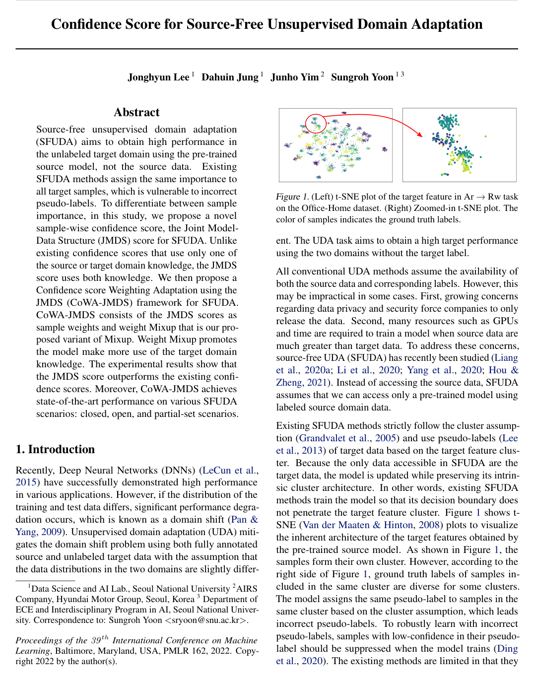
In Source-Free Unsupervised Domain Adaptation (SFUDA), a pre-trained source model $M = g \circ f$ (composed of feature extractor $f: \mathcal{X} \to \mathbb{R}^d$ and classifier $g: \mathbb{R}^d \to \mathbb{R}^K$ ) is adapted to unlabeled target data $X_t = \{x_i^t\}_{i=1}^{n_t}$ without accessing source domain data. Existing confidence scores rely exclusively on either source model predictions or target feature clustering. The Joint Model-Data Structure (JMDS) score combines source-domain model knowledge with target-domain geometric data structure knowledge to assign sample-wise confidence weights $\text{JMDS}(x_i^t) \in [0, 1]$ .

The JMDS score is defined as the product of two constituent scores:

$\text{JMDS}(x_i^t) = \text{LPG}(x_i^t) \cdot \text{MPPL}(x_i^t)$
1. Log-Probability Gap (LPG) score (data-structure-wise confidence): Let $p_{\text{data}}(x_i^t) \in \mathbb{R}^K$ be the posterior class probability distribution derived by fitting a Gaussian Mixture Model (GMM) on target feature representations $\{f(x_i^t)\}_{i=1}^{n_t}$ , and let $\hat{y}_i^t = \arg\max_c p_{\text{data}}(x_i^t)_c$ be the corresponding cluster pseudo-label. The minimum log-probability margin $\text{MINGAP}(x_i^t)$ between the assigned pseudo-label and any rival class $a \neq \hat{y}_i^t$ is computed as:
$\text{MINGAP}(x_i^t) = \min_{a \in \{1, \dots, K\}, a \neq \hat{y}_i^t} \left\{ \log p_{\text{data}}(x_i^t)_{\hat{y}_i^t} - \log p_{\text{data}}(x_i^t)_a \right\}$

Normalizing across all target samples yields the LPG score:

$\text{LPG}(x_i^t) = \frac{\text{MINGAP}(x_i^t)}{\max_{j \in \{1, \dots, n_t\}} \text{MINGAP}(x_j^t)}$

$\text{LPG}(x_i^t)$ assigns high confidence to samples situated far from GMM decision boundaries in the target feature space.
1. Model Probability of Pseudo-Label (MPPL) score (model-wise confidence): Evaluates the pre-trained model's softmax prediction $p_M(x_i^t) = \text{softmax}(g(f(x_i^t)))$ at the GMM-derived pseudo-label $\hat{y}_i^t$ :
$\text{MPPL}(x_i^t) = p_M(x_i^t)_{\hat{y}_i^t}$

Combining LPG and MPPL suppresses overconfident predictions from deep neural network classifiers (which often produce high confidence even on misclassified out-of-distribution target samples) while also penalizing samples located near the source classifier's decision boundaries.
Knowl 2 — Gaussian Mixture Modeling for Feature-Space Pseudo-Labeling
model/method
In the target feature space $\{f(x_i^t)\}_{i=1}^{n_t} \subset \mathbb{R}^d$ , a Gaussian Mixture Model with $K$ components is parameterized by mixing coefficients $\pi_c$ , mean vectors $\mu_c \in \mathbb{R}^d$ , and covariance matrices $\Sigma_c \in \mathbb{R}^{d \times d}$ for each class $c \in \{1, \dots, K\}$ . The conditional log-likelihood of a target feature $f(x_i^t)$ under class component $c$ is:

$\log p(x_i^t \mid \mu_c, \Sigma_c) = -\frac{1}{2} \left( d \log(2\pi) + \log |\Sigma_c| + (f(x_i^t) - \mu_c)^T \Sigma_c^{-1} (f(x_i^t) - \mu_c) \right)$

The data-structure-wise posterior class assignment probability $p_{\text{data}}(x_i^t)_c$ is:

$p_{\text{data}}(x_i^t)_c = \frac{\pi_c p(x_i^t \mid \mu_c, \Sigma_c)}{\sum_{c'=1}^K \pi_{c'} p(x_i^t \mid \mu_{c'}, \Sigma_{c'})}$

The pseudo-label $\hat{y}_i^t$ is assigned by the maximum posterior probability:

$\hat{y}_i^t = \arg\max_{c \in \{1, \dots, K\}} p_{\text{data}}(x_i^t)_c$

To prevent numerical instability when estimating covariance matrices in high-dimensional feature spaces, GMM parameters $\{\pi_c, \mu_c, \Sigma_c\}_{c=1}^K$ are initialized using the model predictive probabilities $p_M(X_t)$ , and a single Expectation-Maximization (EM) iteration is executed per update.
Knowl 3 — Weight Mixup for Confidence-Aware Data Augmentation
model/method
Direct sample-weighting in SFUDA downweights low-confidence samples to near-zero importance, which risks underutilizing target domain geometric information. Weight Mixup resolves this by interpolating input images, one-hot pseudo-labels, and their sample-wise JMDS confidence scores simultaneously.

Given two target samples $(x_i^t, \hat{y}_i^t)$ and $(x_j^t, \hat{y}_j^t)$ with corresponding confidence weights $\text{JMDS}(x_i^t)$ and $\text{JMDS}(x_j^t)$ , the mixed input $\tilde{x}^t$ , mixed target label $\tilde{y}^t$ , and mixed confidence weight $w(\tilde{x}^t)$ are constructed as:

$\tilde{x}^t = \gamma x_i^t + (1 - \gamma) x_j^t$

$\tilde{y}^t = \gamma o(\hat{y}_i^t) + (1 - \gamma) o(\hat{y}_j^t)$

$w(\tilde{x}^t) = \gamma \text{JMDS}(x_i^t) + (1 - \gamma) \text{JMDS}(x_j^t)$

where $\gamma \sim \text{Beta}(\alpha, \alpha)$ with hyperparameter $\alpha \in (0, \infty)$ , and $o(\cdot)$ represents the one-hot encoding function.

The Weight Mixup loss function is the confidence-weighted cross-entropy on the interpolated samples:

$\mathcal{L}_{\text{Mixup}}(\tilde{x}^t, \tilde{y}^t) = w(\tilde{x}^t) \cdot \mathbb{E}_{\tilde{y}^t} [-\log p_M(\tilde{x}^t)] = -w(\tilde{x}^t) \sum_{c=1}^K \tilde{y}_c^t \log p_M(\tilde{x}^t)_c$

When a low-confidence sample is blended with a high-confidence sample, the resulting virtual instance obtains a moderate confidence weight and participates productively in training. Conversely, mixing two low-confidence samples yields a low weight, preventing confirmation bias from noisy pseudo-labels.
Knowl 4 — Confidence Score Weighting Adaptation (CoWA-JMDS) Algorithm
algorithm
The Confidence Score Weighting Adaptation using JMDS (CoWA-JMDS) framework fine-tunes a pre-trained source model $M = g \circ f$ on unlabeled target data $X_t = \{x_i^t\}_{i=1}^{n_t}$ by weighting pseudo-label supervision via JMDS scores and applying Weight Mixup.
Input: Unlabeled target data $X_t$ , pre-trained source model $M = g \circ f$ , maximum epochs $E$ , iterations per epoch $I$ , Mixup parameter $\alpha$
epoch $\leftarrow 0$
repeat
    if partial-set scenario then
        Estimate active class subset $C_{partial}$ via GMM class pruning
    end if
    Extract target features $f(X_t)$ using feature extractor $f$
    Fit GMM on $f(X_t)$ to obtain data-structure probabilities $p_{\text{data}}(X_t)$ and pseudo-labels $\hat{Y}_t$
    if open-set scenario then
        Partition $X_t$ into known cluster $C_{\text{known}}$ and unknown cluster $C_{\text{unknown}}$ by 2-class k-means on the entropy of $p_M(X_t)$
    end if
    Compute sample-wise JMDS scores $\text{JMDS}(x_i^t) = \text{LPG}(x_i^t) \cdot \text{MPPL}(x_i^t)$ for all samples
    for iter $\leftarrow 1$ to $I$ do
        Sample mini-batch from $X_t$ (restricted to $C_{\text{known}}$ in open-set)
        if Weight Mixup is enabled then
            Sample $\gamma \sim \text{Beta}(\alpha, \alpha)$
            Form $\tilde{x}^t = \gamma x_i^t + (1 - \gamma) x_j^t$ , $\tilde{y}^t = \gamma o(\hat{y}_i^t) + (1 - \gamma) o(\hat{y}_j^t)$ , and $w(\tilde{x}^t) = \gamma \text{JMDS}(x_i^t) + (1 - \gamma) \text{JMDS}(x_j^t)$
            Compute loss $\mathcal{L} = \frac{1}{B} \sum_{b=1}^B \mathcal{L}_{\text{Mixup}}(\tilde{x}_b^t, \tilde{y}_b^t)$
        else
            Compute loss $\mathcal{L} = -\frac{1}{B} \sum_{b=1}^B \text{JMDS}(x_b^t) \log p_M(x_b^t)_{\hat{y}_b^t}$
        end if
        Update model parameters $M$ by gradient descent on $\mathcal{L}$
    end for
    epoch $\leftarrow$ epoch $+ 1$
until epoch $\ge E$
Output: Adapted target model $M$
Optimization is performed with mini-batch SGD (momentum 0.9, weight decay $1\times 10^{-3}$ , batch size 64). The bottleneck layer uses learning rate $1\times 10^{-2}$ while the rest of the network uses $1\times 10^{-3}$ without learning rate decay. Total training epochs are 50 (Office-31), 30 (Office-Home), and 15 (VisDA-2017), with $\alpha = 0.2$ for Office-31/Office-Home and $\alpha = 2.0$ for VisDA-2017.
Knowl 5 — Class Estimation and Filtering for Open-Set and Partial-Set SFUDA
algorithm
CoWA-JMDS adapts to open-set and partial-set scenarios via specialized sample and class filtering procedures prior to GMM fitting:

1. Open-Set SFUDA (Target domain contains unknown classes not present in source): Known and unknown target instances are separated using the predictive entropy of the pre-trained model $p_M(X_t)$ . Entropy values $H(p_M(x_i^t)) = -\sum_{c=1}^K p_M(x_i^t)_c \log p_M(x_i^t)_c$ are clustered into two partitions using 2-class $k$ -means. The low-entropy partition $C_{\text{low-entropy}}$ is designated as known-class samples and used for model adaptation, while the high-entropy partition $C_{\text{high-entropy}}$ is classified as unknown classes.

2. Partial-Set SFUDA (Target domain contains only a subset of source classes): Absent classes are filtered out iteratively via thresholding on cumulative GMM posterior probabilities:
Input: Unlabeled target data $X_t$ , model $M = g \circ f$ , pruning threshold $\tau$
Initialize candidate class set $C_{partial} \leftarrow \{c_1, \dots, c_K\}$
repeat
    Initialize GMM parameters $\pi, \mu, \Sigma$ using $p_M(X_t)$ restricted to $C_{partial}$
    Perform one EM iteration of GMM
    Compute data-structure probabilities $p_{\text{data}}(X_t)$ over classes in $C_{partial}$
    for each class $c_j \in C_{partial}$ do
        if $\sum_{i=1}^{n_t} p_{\text{data}}(x_i^t)_{c_j} < \tau \cdot \frac{n_t}{|C_{partial}|}$ then
             $C_{partial} \leftarrow C_{partial} \setminus \{c_j\}$
        end if
    end for
until $C_{partial}$ does not change
Output: Target class set $C_{partial}$
For the Office-Home dataset, the threshold $\tau$ is set to $0.3$ .

Knowl 6 — AURC Evaluation of Pseudo-Label Confidence Estimation

data/table

The quality of confidence scores on the pre-trained source model prior to adaptation is evaluated using the Area Under Risk-Coverage curve (AURC) with 0/1 misclassification loss. Risk is the empirical error rate on the retained high-confidence set $X_t^h = \{x_i^t \mid \kappa(x_i^t, \hat{y}_i^t) > \tau\}$ , and coverage is $|X_t^h| / |X_t|$ . A lower AURC value indicates higher reliability.

Dataset	Task	Naïve PL+Maxprob	Naïve PL+Ent	SSPL+Cossim	GMM+Cossim	GMM+MPPL	GMM+LPG	GMM+JMDS
Office-31	A $\to$ D	0.047	0.051	0.018	0.031	0.039	0.033	0.033
Office-31	A $\to$ W	0.074	0.081	0.034	0.045	0.059	0.042	0.044
Office-31	D $\to$ A	0.158	0.165	0.140	0.130	0.131	0.127	0.115
Office-31	D $\to$ W	0.007	0.008	0.009	0.009	0.005	0.004	0.004
Office-31	W $\to$ A	0.157	0.167	0.107	0.108	0.132	0.120	0.113
Office-31	W $\to$ D	0.002	0.002	0.001	0.001	0.001	0.001	0.001
Office-31	Avg.	0.074	0.079	0.052	0.054	0.061	0.055	0.052
Office-Home	Avg.	0.192	0.200	0.166	0.162	0.169	0.168	0.151
VisDA-2017	T $\to$ V	0.274	0.284	0.261	0.202	0.204	0.172	0.162

GMM+JMDS achieves the lowest AURC across benchmarks (0.052 on Office-31, 0.151 on Office-Home, and 0.162 on VisDA-2017), demonstrating that jointly combining model prediction probabilities (MPPL) and feature clustering likelihoods (LPG) provides superior confidence discrimination compared to either metric in isolation or standard baselines (Maxprob, negative entropy, cosine similarity).

Knowl 7 — Closed-Set SFUDA Benchmark Performance on Office-31, Office-Home, and VisDA-2017

data/table

Classification accuracy (%) of CoWA-JMDS and competing SFUDA and UDA methods under closed-set conditions on Office-31 (ResNet-50), Office-Home (ResNet-50), and VisDA-2017 (ResNet-101), averaged across 5 random seeds:

Office-31 (ResNet-50)
Type	Method	A $\to$ D	A $\to$ W	D $\to$ A	D $\to$ W	W $\to$ A	W $\to$ D	Avg.
SFUDA	SFIT	89.9	91.8	73.9	98.7	72.0	99.9	87.7
SFUDA	SHOT	94.0	90.1	74.7	98.4	74.3	99.9	88.6
SFUDA	3C-GAN	92.7	93.7	75.3	98.5	77.8	99.8	89.6
SFUDA	NRC	96.0	90.8	75.3	99.0	75.0	100.0	89.4
SFUDA	CoWA-JMDS (w/o weight Mixup)	93.7	93.5	75.5	98.0	76.8	99.8	89.6
SFUDA	CoWA-JMDS	94.4	95.2	76.2	98.5	77.6	99.8	90.3
UDA	ResNet-50	68.9	68.4	62.5	96.7	60.7	99.3	76.1
UDA	CAN	95.0	94.5	78.0	99.1	77.0	99.8	90.6

On Office-Home (12 adaptation tasks among Art, Clipart, Product, Real-World), average accuracy is:

SFUDA baselines: BAIT (71.6%), SHOT (71.8%), NRC (72.2%).
CoWA-JMDS (w/o weight Mixup): 72.2%.
CoWA-JMDS (full): 72.5% (Task accuracies: Ar $\to$ Cl: 56.9%, Ar $\to$ Pr: 78.4%, Ar $\to$ Rw: 81.0%, Cl $\to$ Ar: 69.1%, Cl $\to$ Pr: 80.0%, Cl $\to$ Rw: 79.9%, Pr $\to$ Ar: 67.7%, Pr $\to$ Cl: 57.2%, Pr $\to$ Rw: 82.4%, Rw $\to$ Ar: 72.8%, Rw $\to$ Cl: 60.5%, Rw $\to$ Pr: 84.5%).

On VisDA-2017 (Synthetic $\to$ Real, 12 classes):

SFUDA baselines: SFIT (81.4%), 3C-GAN (81.6%), SHOT (82.9%), NRC (85.9%).
CoWA-JMDS (w/o weight Mixup): 84.2%.
CoWA-JMDS (full): 86.9% (plane: 96.2%, bcycl: 89.7%, bus: 83.9%, car: 73.8%, horse: 96.4%, knife: 97.4%, mcycl: 89.3%, person: 86.8%, plant: 94.6%, sktbrd: 92.1%, train: 88.7%, truck: 53.8%).

Knowl 8 — Open-Set and Partial-Set SFUDA Benchmark Performance on Office-Home

data/table

Classification accuracy (%) on the Office-Home dataset across open-set (source: 25 classes, target: 65 classes including unknown) and partial-set (source: 65 classes, target: 25 classes) scenarios using ResNet-50:

Open-Set SFUDA on Office-Home
Type	Method	Ar $\to$ Cl	Ar $\to$ Pr	Ar $\to$ Rw	Cl $\to$ Ar	Cl $\to$ Pr	Cl $\to$ Rw	Pr $\to$ Ar	Pr $\to$ Cl	Pr $\to$ Rw	Rw $\to$ Ar	Rw $\to$ Cl	Rw $\to$ Pr	Avg.
SFUDA	SHOT	64.5	80.4	84.7	63.1	75.4	81.2	65.3	59.3	83.3	69.6	64.6	82.3	72.8
SFUDA	CoWA-JMDS (w/o mixup)	64.6	80.2	88.1	67.3	83.5	82.2	63.9	57.1	84.4	70.8	64.0	84.8	74.2
SFUDA	CoWA-JMDS	63.3	79.2	85.4	67.6	83.6	82.0	66.9	56.9	81.1	68.5	57.9	85.9	73.2
UDA	STA	58.1	53.1	54.4	71.6	69.3	81.9	63.4	65.2	74.9	85.0	75.8	80.8	69.5
UDA	PGL	61.6	77.1	85.9	68.8	72.0	82.8	72.2	58.4	82.6	78.6	65.0	83.0	74.0
Partial-Set SFUDA on Office-Home
SFUDA	SHOT	64.8	85.2	92.7	76.3	77.6	88.8	79.7	64.3	89.5	80.6	66.4	85.8	79.3
SFUDA	CoWA-JMDS (w/o mixup)	69.7	91.6	92.1	78.9	86.3	91.6	81.5	64.4	89.7	84.1	71.6	90.2	82.6
SFUDA	CoWA-JMDS	69.6	93.2	92.3	78.9	81.3	92.1	79.8	71.7	90.0	83.8	72.2	93.7	83.2
UDA	SAFN	58.9	76.3	81.4	70.4	73.0	77.8	72.4	55.3	80.4	75.8	60.4	79.9	71.8
UDA	BA $^3$ US	60.6	83.1	88.4	71.8	72.8	83.4	75.5	61.6	86.5	79.3	62.8	86.1	76.0

In the partial-set scenario, full CoWA-JMDS achieves state-of-the-art accuracy of 83.2%, outperforming SHOT (79.3%) and UDA methods. In the open-set scenario, CoWA-JMDS without Weight Mixup achieves the highest performance (74.2%); applying Weight Mixup in open-set settings reduces accuracy to 73.2% because mixing misclassified unknown instances into known classes introduces label corruption.

Knowl 9 — Ablation of Weight Mixup against Standard Mixup in SFUDA

data/table

The effectiveness of Weight Mixup compared to standard Mixup and pseudo-labeling baselines is evaluated on the Office-31 dataset:

Applying standard Mixup yields only marginal performance gains (+0.2% on SHOT, +0.3% on GMM pseudo-labels) because standard Mixup weights all interpolated samples equally, exacerbating confirmation bias from incorrect pseudo-labels. In contrast, Weight Mixup scales the training objective by the blended JMDS confidence score, delivering a +3.4% accuracy improvement over GMM PL + Mixup (86.9% $\to$ 90.3%) and a +0.7% boost over GMM PL + JMDS without mixup (89.6% $\to$ 90.3%).

Knowl 10 — Progressive Learning Dynamics and Underfitting Prevention in CoWA-JMDS
empirical result
At epoch 0 (prior to adaptation), target feature representations contain substantial ambiguity, causing a significant fraction of target samples to receive low JMDS confidence scores (e.g., $< 0.2$ ). While static low weights could cause underfitting, the dynamic re-estimation of JMDS scores across training epochs exhibits self-paced/curriculum learning behavior.

As the feature extractor $f$ and classifier $g$ are updated, feature cluster separation improves and aligns with decision boundaries. Consequently, empirical quantile distributions of JMDS scores systematically shift upward across successive training epochs (epochs 1, 2, 10, 30, and 50). This progressive increase in sample confidence ensures that initially suppressed low-confidence samples gradually gain higher weights and participate fully in adaptation, preventing underfitting without requiring heuristic hard-threshold sample pruning.

Coverage note — None was omitted; all key theoretical formulations (JMDS, LPG, MPPL, Weight Mixup), algorithms (CoWA-JMDS, open-set and partial-set filtering), and empirical evaluations (AURC, closed/open/partial-set benchmarks, ablation studies, and learning dynamics) from the paper are represented.

References

1.Arazo, E., Ortego, D., Albert, P., O’Connor, N. E., and McGuinness, K. Pseudo-labeling and confirmation bias in deep semi-supervised learning. In 2020 International Joint Conference on Neural Networks (IJCNN), pp. 1–8. IEEE, 2020.
2.Bengio, Y., Louradour, J., Collobert, R., and Weston, J. Curriculum learning. In Proceedings of the 26th annual international conference on machine learning, pp. 41–48, 2009.
3.Cao, Z., Long, M., Wang, J., and Jordan, M. I. Partial transfer learning with selective adversarial networks. In Proceedings of the IEEE conference on computer vision and pattern recognition, pp. 2724–2732, 2018.
4.Ding, Y., Liu, J., Xiong, J., and Shi, Y. Revisiting the evaluation of uncertainty estimation and its application to explore model complexity-uncertainty trade-off. In Proceedings of the IEEE/CVF Conference on Computer Vision and Pattern Recognition Workshops, pp. 4–5, 2020.
5.Geifman, Y. and El-Yaniv, R. Selective classification for deep neural networks. arXiv preprint arXiv:1705.08500, 2017.
6.Geifman, Y., Uziel, G., and El-Yaniv, R. Bias-reduced uncertainty estimation for deep neural classifiers. arXiv preprint arXiv:1805.08206, 2018.
7.Grandvalet, Y., Bengio, Y., et al. Semi-supervised learning by entropy minimization. CAP, 367:281–296, 2005.
8.Gu, X., Sun, J., and Xu, Z. Spherical space domain adaptation with robust pseudo-label loss. In Proceedings of the IEEE/CVF Conference on Computer Vision and Pattern Recognition, pp. 9101–9110, 2020.
9.He, K., Zhang, X., Ren, S., and Sun, J. Deep residual learning for image recognition. In Proceedings of the IEEE conference on computer vision and pattern recognition, pp. 770–778, 2016.
10.Hein, M., Andriushchenko, M., and Bitterwolf, J. Why relu networks yield high-confidence predictions far away from the training data and how to mitigate the problem. In Proceedings of the IEEE/CVF Conference on Computer Vision and Pattern Recognition, pp. 41–50, 2019.
11.Hou, Y. and Zheng, L. Visualizing adapted knowledge in domain transfer. In Proceedings of the IEEE/CVF Conference on Computer Vision and Pattern Recognition, pp. 13824–13833, 2021.
12.Ioffe, S. and Szegedy, C. Batch normalization: Accelerating deep network training by reducing internal covariate shift. In International conference on machine learning, pp. 448–456. PMLR, 2015.
13.Kang, G., Jiang, L., Yang, Y., and Hauptmann, A. G. Contrastive adaptation network for unsupervised domain adaptation. In Proceedings of the IEEE Conference on Computer Vision and Pattern Recognition, pp. 4893–4902, 2019.
14.Kumar, M. P., Packer, B., and Koller, D. Self-paced learning for latent variable models. In NIPS, volume 1, pp. 2, 2010.
15.Lakshminarayanan, B., Pritzel, A., and Blundell, C. Simple and scalable predictive uncertainty estimation using deep ensembles. arXiv preprint arXiv:1612.01474, 2016.
16.Langley, P. Crafting papers on machine learning. In Langley, P. (ed.), Proceedings of the 17th International Conference on Machine Learning (ICML 2000), pp. 1207–1216, Stanford, CA, 2000. Morgan Kaufmann.
17.LeCun, Y., Bengio, Y., and Hinton, G. Deep learning. nature, 521(7553):436–444, 2015.
18.Lee, D.-H. et al. Pseudo-label: The simple and efficient semi-supervised learning method for deep neural networks. In Workshop on challenges in representation learning, ICML, 2013.
19.Lee, K., Lee, K., Lee, H., and Shin, J. A simple unified framework for detecting out-of-distribution samples and adversarial attacks. Advances in neural information processing systems, 31, 2018.
20.Li, R., Jiao, Q., Cao, W., Wong, H.-S., and Wu, S. Model adaptation: Unsupervised domain adaptation without source data. In Proceedings of the IEEE/CVF Conference on Computer Vision and Pattern Recognition, pp. 9641–9650, 2020.
21.Liang, J., Hu, D., and Feng, J. Do we really need to access the source data? source hypothesis transfer for unsupervised domain adaptation. In International Conference on Machine Learning, pp. 6028–6039. PMLR, 2020a.
22.Liang, J., Wang, Y., Hu, D., He, R., and Feng, J. A balanced and uncertainty-aware approach for partial domain adaptation. In Computer Vision–ECCV 2020: 16th European Conference, Glasgow, UK, August 23–28, 2020, Proceedings, Part XI 16, pp. 123–140. Springer, 2020b.
23.Liu, H., Cao, Z., Long, M., Wang, J., and Yang, Q. Separate to adapt: Open set domain adaptation via progressive separation. In Proceedings of the IEEE/CVF Conference on Computer Vision and Pattern Recognition, pp. 2927–2936, 2019.
24.Luo, Y., Wang, Z., Huang, Z., and Baktashmotlagh, M. Progressive graph learning for open-set domain adaptation. In International Conference on Machine Learning, pp. 6468–6478. PMLR, 2020.
25.Mandelbaum, A. and Weinshall, D. Distance-based confidence score for neural network classifiers. arXiv preprint arXiv:1709.09844, 2017.
26.Müller, R., Kornblith, S., and Hinton, G. When does label smoothing help? arXiv preprint arXiv:1906.02629, 2019.
27.Na, J., Jung, H., Chang, H., and Hwang, W. Fixbi: Bridging domain spaces for unsupervised domain adaptation. arXiv preprint arXiv:2011.09230, 2020.
28.Nair, T., Precup, D., Arnold, D. L., and Arbel, T. Exploring uncertainty measures in deep networks for multiple sclerosis lesion detection and segmentation. Medical image analysis, 59:101557, 2020.
29.Pan, S. J. and Yang, Q. A survey on transfer learning. IEEE Transactions on knowledge and data engineering, 22(10): 1345–1359, 2009.
30.Panareda Busto, P. and Gall, J. Open set domain adaptation. In Proceedings of the IEEE International Conference on Computer Vision, pp. 754–763, 2017.
31.Peng, X., Usman, B., Kaushik, N., Hoffman, J., Wang, D., and Saenko, K. Visda: The visual domain adaptation challenge. arXiv preprint arXiv:1710.06924, 2017.
32.Ren, M., Zeng, W., Yang, B., and Urtasun, R. Learning to reweight examples for robust deep learning. In International Conference on Machine Learning, pp. 4334–4343. PMLR, 2018.
33.Saenko, K., Kulis, B., Fritz, M., and Darrell, T. Adapting visual category models to new domains. In European conference on computer vision, pp. 213–226. Springer, 2010.
34.Salimans, T. and Kingma, D. P. Weight normalization: A simple reparameterization to accelerate training of deep neural networks. arXiv preprint arXiv:1602.07868, 2016.
35.Tang, H., Chen, K., and Jia, K. Unsupervised domain adaptation via structurally regularized deep clustering. In Proceedings of the IEEE/CVF conference on computer vision and pattern recognition, pp. 8725–8735, 2020.
36.Van der Maaten, L. and Hinton, G. Visualizing data using t-sne. Journal of machine learning research, 9(11), 2008.
37.Venkateswara, H., Eusebio, J., Chakraborty, S., and Panchanathan, S. Deep hashing network for unsupervised domain adaptation. In Proceedings of the IEEE conference on computer vision and pattern recognition, pp. 5018–5027, 2017.
38.Xu, R., Li, G., Yang, J., and Lin, L. Larger norm more transferable: An adaptive feature norm approach for unsupervised domain adaptation. In Proceedings of the IEEE/CVF International Conference on Computer Vision, pp. 1426–1435, 2019.
39.Yang, S., Wang, Y., van de Weijer, J., Herranz, L., and Jui, S. Unsupervised domain adaptation without source data by casting a bait. arXiv preprint arXiv:2010.12427, 2020.
40.Yang, S., van de Weijer, J., Herranz, L., Jui, S., et al. Exploiting the intrinsic neighborhood structure for source-free domain adaptation. Advances in Neural Information Processing Systems, 34, 2021.
41.Zhang, H., Cisse, M., Dauphin, Y. N., and Lopez-Paz, D. mixup: Beyond empirical risk minimization. arXiv preprint arXiv:1710.09412, 2017.

Citation

MLA

Lee, J., et al. “Confidence Score for Source-Free Unsupervised Domain Adaptation”. International Conference on Machine Learning, vol. 162, 2022, pp. 12365–77, https://proceedings.mlr.press/v162/lee22c.html.

APA

Lee, J., Jung, D., Yim, J., & Yoon, S. (2022). Confidence Score for Source-Free Unsupervised Domain Adaptation. International Conference on Machine Learning, 162, 12365–12377. https://proceedings.mlr.press/v162/lee22c.html

Chicago

Lee, J., D. Jung, J. Yim, and S. Yoon. 2022. “Confidence Score for Source-Free Unsupervised Domain Adaptation”. International Conference on Machine Learning 162: 12365–77. https://proceedings.mlr.press/v162/lee22c.html.

Harvard

Lee, J. et al. (2022) “Confidence Score for Source-Free Unsupervised Domain Adaptation”, International Conference on Machine Learning. PMLR, pp. 12365–12377. Available at: https://proceedings.mlr.press/v162/lee22c.html.

Vancouver

1. Lee J, Jung D, Yim J, Yoon S (2022) Confidence Score for Source-Free Unsupervised Domain Adaptation. In: International Conference on Machine Learning. PMLR, pp 12365–12377

BibTeX

@InProceedings{pmlr-v162-lee22c,
  title = 	 {Confidence Score for Source-Free Unsupervised Domain Adaptation},
  author =       {Lee, Jonghyun and Jung, Dahuin and Yim, Junho and Yoon, Sungroh},
  booktitle = 	 {Proceedings of the 39th International Conference on Machine Learning},
  pages = 	 {12365--12377},
  year = 	 {2022},
  editor = 	 {Chaudhuri, Kamalika and Jegelka, Stefanie and Song, Le and Szepesvari, Csaba and Niu, Gang and Sabato, Sivan},
  volume = 	 {162},
  series = 	 {Proceedings of Machine Learning Research},
  month = 	 {17--23 Jul},
  publisher =    {PMLR},
  pdf = 	 {https://proceedings.mlr.press/v162/lee22c/lee22c.pdf},
  url = 	 {https://proceedings.mlr.press/v162/lee22c.html},
  abstract = 	 {Source-free unsupervised domain adaptation (SFUDA) aims to obtain high performance in the unlabeled target domain using the pre-trained source model, not the source data. Existing SFUDA methods assign the same importance to all target samples, which is vulnerable to incorrect pseudo-labels. To differentiate between sample importance, in this study, we propose a novel sample-wise confidence score, the Joint Model-Data Structure (JMDS) score for SFUDA. Unlike existing confidence scores that use only one of the source or target domain knowledge, the JMDS score uses both knowledge. We then propose a Confidence score Weighting Adaptation using the JMDS (CoWA-JMDS) framework for SFUDA. CoWA-JMDS consists of the JMDS scores as sample weights and weight Mixup that is our proposed variant of Mixup. Weight Mixup promotes the model make more use of the target domain knowledge. The experimental results show that the JMDS score outperforms the existing confidence scores. Moreover, CoWA-JMDS achieves state-of-the-art performance on various SFUDA scenarios: closed, open, and partial-set scenarios.}
}

Metadata:DOI registry

Source Code

This paper has an official code repository available. Click below to access the source code.

View Repository

Access the Paper

This paper is available from its original source. Click below to access the PDF.

Open PDF

License: https://creativecommons.org/licenses/by/4.0/

Method	Average Accuracy (%)
SHOT	88.6
SHOT + Mixup	88.8
GMM PL	86.6
GMM PL + Mixup	86.9
GMM PL + JMDS	89.6
GMM PL + JMDS + Weight Mixup (CoWA-JMDS)	90.3

Confidence Score for Source-Free Unsupervised Domain Adaptation

Abstract

Topics

Keywords

Table of Contents

Knowls

Knowl 1 — Joint Model-Data Structure Confidence Score

Knowl 2 — Gaussian Mixture Modeling for Feature-Space Pseudo-Labeling

Knowl 3 — Weight Mixup for Confidence-Aware Data Augmentation

Knowl 4 — Confidence Score Weighting Adaptation (CoWA-JMDS) Algorithm

Knowl 5 — Class Estimation and Filtering for Open-Set and Partial-Set SFUDA

Knowl 6 — AURC Evaluation of Pseudo-Label Confidence Estimation

Knowl 7 — Closed-Set SFUDA Benchmark Performance on Office-31, Office-Home, and VisDA-2017

Knowl 8 — Open-Set and Partial-Set SFUDA Benchmark Performance on Office-Home

Knowl 9 — Ablation of Weight Mixup against Standard Mixup in SFUDA

Knowl 10 — Progressive Learning Dynamics and Underfitting Prevention in CoWA-JMDS

References

Citation

BibTeX

Source Code

Access the Paper